Article

HCTNav: A Path Planning Algorithm for Low-Cost Autonomous Robot Navigation in Indoor Environments

Human Computer Technology Laboratory, EPS, Universidad Autónoma de Madrid. Francisco Tomás y Valiente 11, E-28049 Madrid, Spain
*
Author to whom correspondence should be addressed.
ISPRS Int. J. Geo-Inf. 2013, 2(3), 729-748; https://doi.org/10.3390/ijgi2030729
Submission received: 25 June 2013 / Revised: 29 July 2013 / Accepted: 31 July 2013 / Published: 9 August 2013
(This article belongs to the Special Issue Indoor Positioning and Indoor Navigation)

Abstract

:
Low-cost robots are characterized by low computational resources and limited energy supply. Path planning algorithms aim to find the optimal path between two points so the robot consumes as little energy as possible. However, these algorithms were not developed considering computational limitations (i.e., processing and memory capacity). This paper presents the HCTNav path-planning algorithm (HCTLab research group’s navigation algorithm). This algorithm was designed to be run in low-cost robots for indoor navigation. The results of the comparison between HCTNav and the Dijkstra’s algorithms show that HCTNav’s memory peak is nine times lower than Dijkstra’s in maps with more than 150,000 cells.

Graphical Abstract

1. Introduction

The path-planning efficiency for the autonomous robot navigation problem is still an open challenge in robotics. In the last two decades, the efforts to reach an intelligent motion behavior, suitable for robotic vehicles, lead to two of the most-known approaches in literature and industry: the deterministic solution, based on heuristic graph search, and the reactive one, based on environment sensor sampling [1]. When choosing between the former approaches, it is important to figure out which performance factor is critical for the real case scenario. For example, the deterministic algorithms offer a very fast execution and the optimum solution, although they are penalized by map scalability; on the other hand, the reactive algorithms are independent to map scaling and can handle dynamic changes, but do not guarantee the minimum path solution [2].
The Dijkstra’s algorithm [3] is the very reference for the deterministic solutions, due to its mathematical robustness when planning the shortest path. Nevertheless, Dijkstra’s approach presents two known problems: (1) spanning the whole search frontier increases the algorithm execution time, resulting in decreased speed performance; (2) dynamic memory usage exhibits quadratic growth, thus requiring a large amount of RAM in massive graphs [4].
To reduce the “overhead problem”, i.e., the unnecessary exploration of map areas that does not lead to the target, many authors have improved Dijkstra’s concept, by adding a heuristic estimation of remaining distance to the target. The estimation applies when choosing the next node from the search frontier. These Dijkstra’s evolutions are known as the A* family (A-star) and they are largely employed to solve the path-planning problem [5]. The Euclidean heuristic [6] uses straight distance as estimation of the remaining distance, whereas the Manhattan heuristic [7] uses the sum of the Cartesian projections of the distance vector. Dijkstra’s algorithms implement an optimum path-search [8] and always return the shortest path, which is why they still continue to represent the first choice in the market of route guidance systems (like GPS navigators) [9], logistic planners [10], and even for autonomous mobile robot navigation [11,12,13].
The reactive approaches can be referenced by the Bugs type algorithms [14], which combine the sensory-based obstacle detection during motion towards the target. These algorithms have evolved in different version through years, starting from the VisBug [15]. The DistBug [16] has improved Bugs’ final-path quality, by adding a set of formal rules to choose the best obstacle surrounding direction and the proper leaving condition during obstacle boundary following.
The most valuable feature for this family is that robots can move in a totally unknown environment, reacting to obstacles according to the proximity sensors information (processed in real-time) [17]. This is known as local convergence approach [18]; despite its performance, this solution does not guarantee the minimum path (because of the local minimum “traps”). In the opposite one, known as global convergence approach [19], the working map will be constructed at a global scope, thus, avoiding the “dead-ends” and providing a better (but not minimal) path, although with a more expensive on-board resources usage.
In this work we present our own algorithm for indoor robot navigation, called HCTNav (HCTLab research group’s navigation algorithm).. The main goal of the algorithm is to find, if it exists, an effective route between two cells in the given binary map, such as the occupancy-grid matrix discussed in González-Arjona et al. [20]. Regarding to performance requirements, the purposes of this research are (1) to increase the scalability in larger maps by controlling the dynamic memory usage at run-time and (2) to grant acceptable execution time. We conceived HCTNav as a hybrid algorithm, combining the graph-search techniques of the deterministic family with the logical rules of the reactive one.
The article is structured as follows: Section 2 describes the environment model and the logical navigation rules; they are the basis for the algorithm discussion in Section 3, which focuses on the HCTNav execution flow and the final path building; the experimental results and the comparison with the state-of-the-art solutions are discussed in Section 4, followed by a brief conclusion.

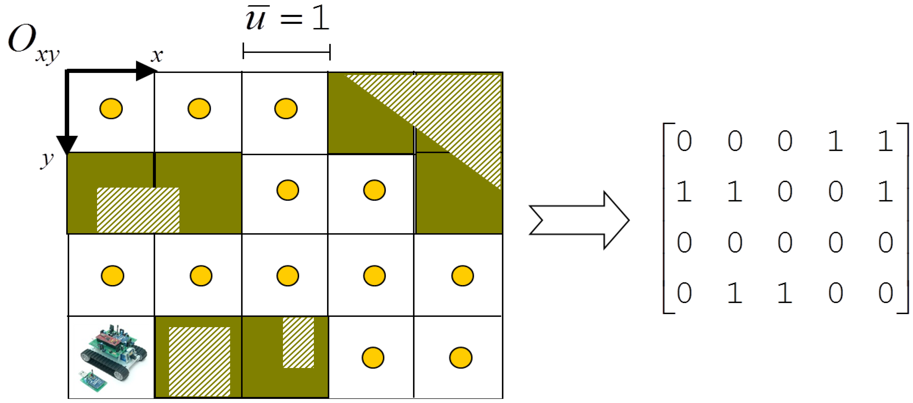
2. Environment and System Model

The HCTNav environment model has been shaped as a two dimensional map. The robot motion is holonomic and as it is limited to indoor areas we assume the ground to be always horizontal. So our scenario falls into the 2D modeling commonly employed in Real-Time Strategy videogames [21]. The terrain is represented by a grid of uniform cells and the movement range is bound to the valid (no obstacles in the trajectory) hops from a cell to another one. Following these principles, the navigation map can be reduced to a logical matrix with entries from the Boolean domain (B := [0,1]). Every cell is identified by its coordinates (x, y) in the matrix. The cell’s status is stored in the correspondent entry: a logical ‘0’ states that the cell is free, whereas a ‘1’ represents an obstructed cell.
The cell is defined by the robot’s size and the robot will always position itself in the geometric center of the cell; thus, any partially occupied cell will be considered an obstructed cell. The tiles’ coordinates belong to the natural numbers domain (N := {0, 1, 2, …} and are in the ranges x ∈ [0, c − 1], y ∈ [0, r − 1], where c represents the number of columns and r the number of rows. The reference is the origin O(x, y), which is fixed in the upper left corner (see Figure 1).
Figure 1. Equivalence between a 2D map and its correspondent binary matrix model. The diagonal-stripes area depicts the real obstacle shapes, whereas the dark tiles are the correspondent obstructed cells. The circles represent all possible coordinates the robot may occupy in the map.
Ijgi 02 00729 g001
So, the resultant navigation data structure represents only the initial graph’s node-set V := {ni} covering the free cells in the 2D grid. Another required abstraction is to normalize the map measure unit to simplify the mathematical notation; in this article we are assuming a cell as a unitary square (l ≡ u =1).

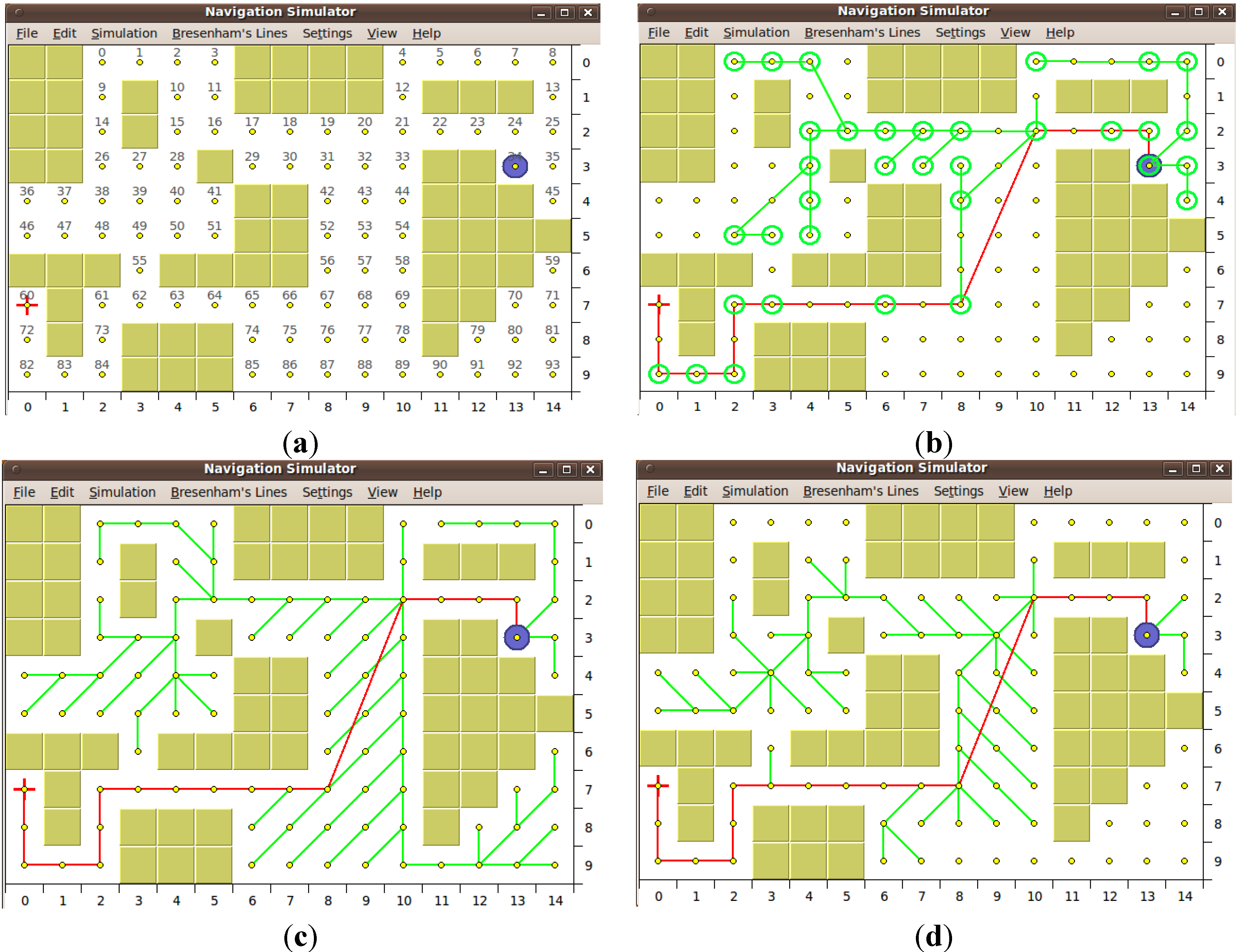
3. The HCTNav Algorithm

In this section we will discuss our algorithm’s processing, by explaining the four main modules that compose the robot’s motion-planning system.
According to our purpose, we started from a set of logical navigation rules inspired on the Bug family movement strategy; that is: try to go straight towards the goal and, in case of obstacles obstructing the way, try to surround them. The Bug approach chooses a surrounding direction, which may not be the optimal. As the HCTNav is executed prior to robot’s movement we may explore in both boundary-following directions. This procedure will create a tree of possible paths from the origin to the destination. Every path is optimized and the shortest one is returned when more than one is found.
The algorithm has been divided into four main modules, each of them fulfills a specific task. The first module implements the obstacle detection in a given straight trajectory (Subsection 3.1); the second one defines the intermediate tile, called turning-point, adjacent to the detected obstacle used to start the surrounding of the obstacle (Subsection 3.2); the third module solves the obstacle surrounding (Subsection 3.3); finally, the fourth one aims at optimizations in the raw navigation graph (by pruning redundant edges) and states the criterion to choose the best path (Subsection 3.4). The initial data structure of the algorithm consists of the elements that model the given map and allow storing the required cell’s properties. The same structure changes all over the execution, as long as HCTNav updates the turning-point list and dynamically builds the intermediate edges.

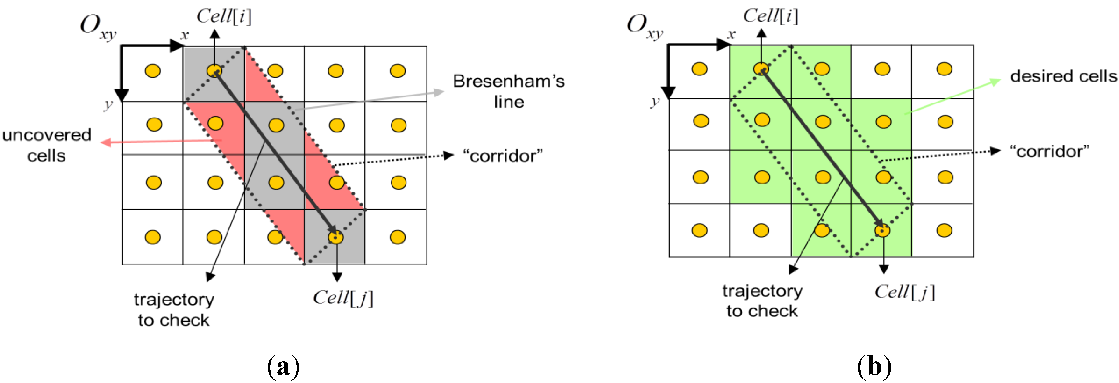
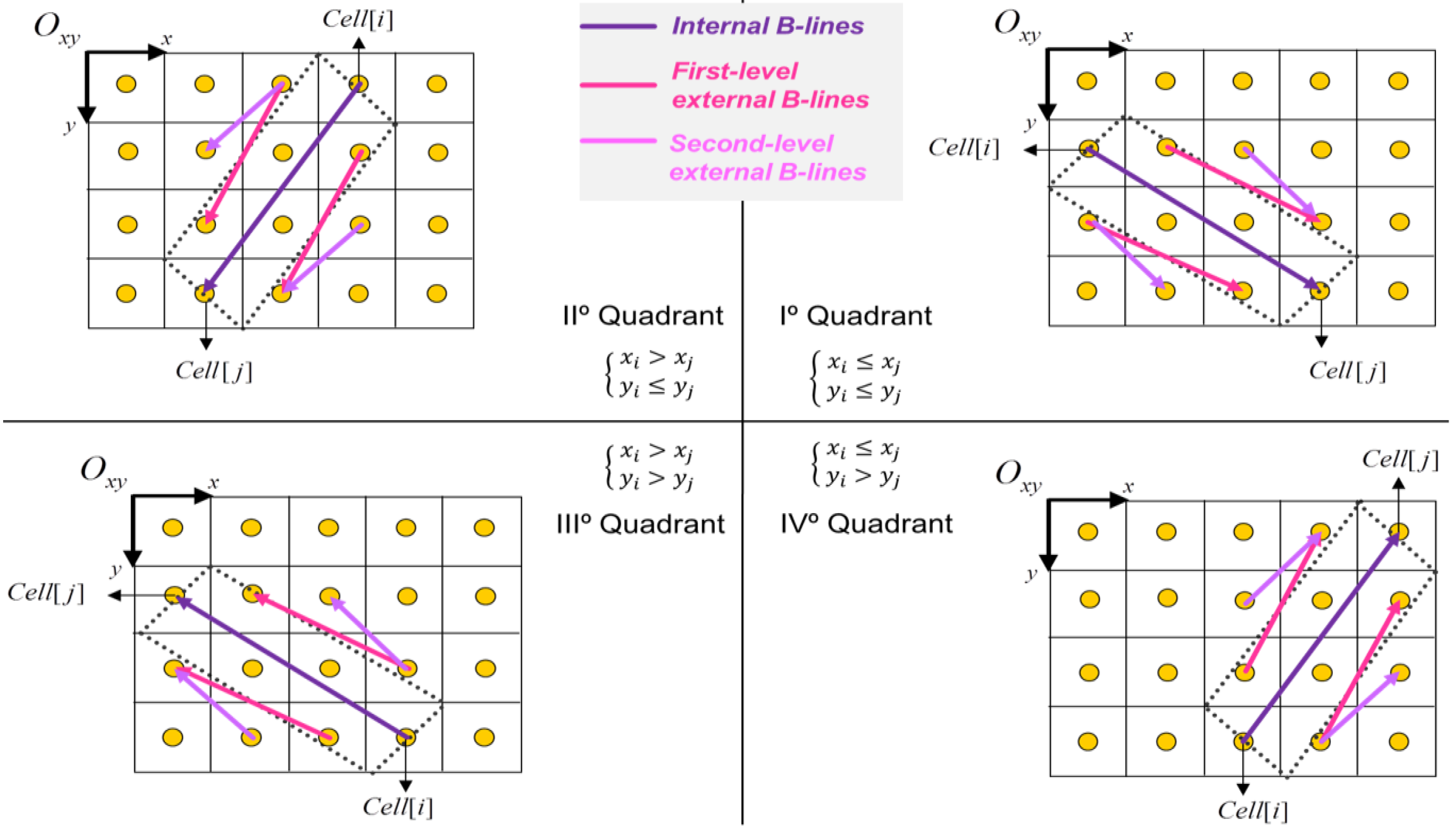
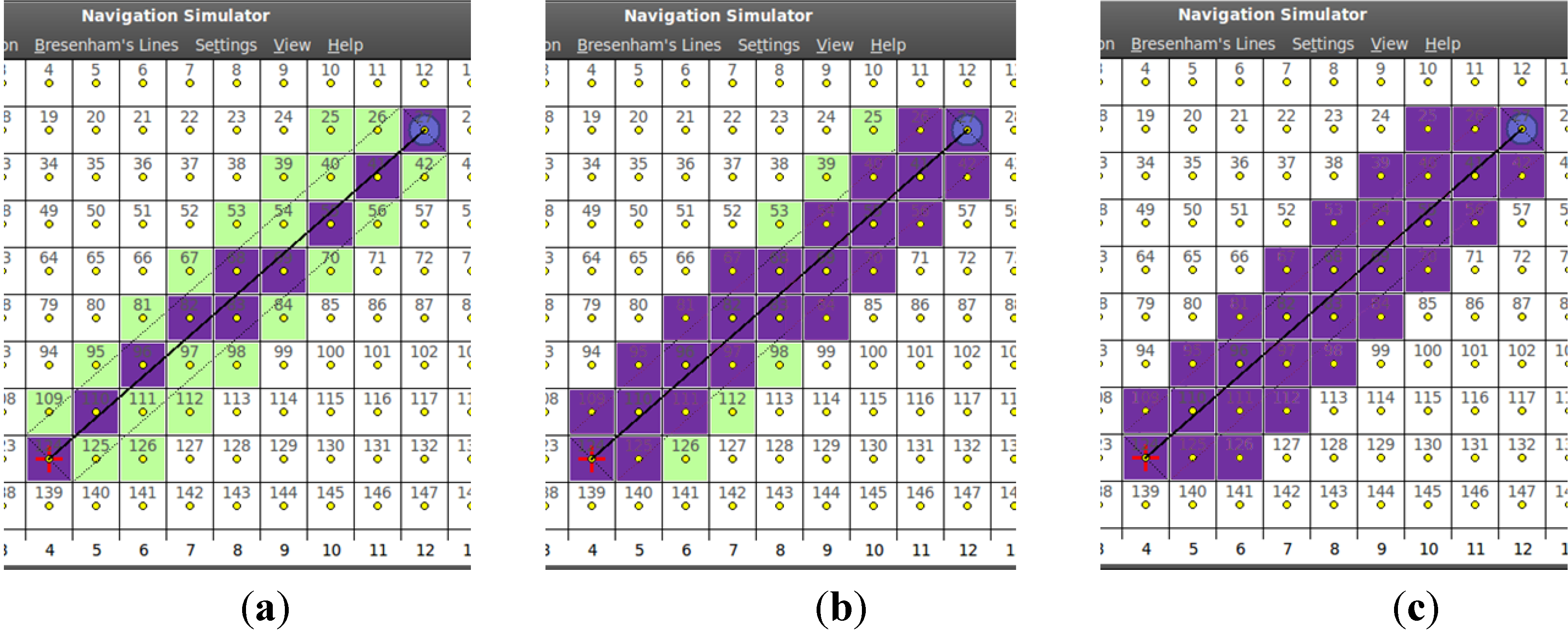
3.1. Obstacle Detection

Given two generic nodes Node[i] and Node[j] in the map, the first module checks if the straight trajectory between them is obstacle-free. If one or more obstacles are found along the way, then the one representing the first “in sight” collision from robot’s perspective will be returned.
The trajectory of the robot can be modeled as a “corridor”, projecting the robot’s front width from the start-point to the end-point; here the goal is to check all the tiles belonging to the corridor to avoid possible collisions (forwarded obstacle detection).
For each cell into the corridor, HCTNav will check and mark all the tiles obstructed (Obstacle[k]) and find the nearest one to the current position. As said, we will consider the square distances from the current Node[i] to Obstacle[k] as d2 (i, k) = (xi − xk)2 + (yi − yk)2, thus avoiding square roots. The module will return the obstacle k such as d2 (i, k*) = mink{d2 (i, k)}, representing the first potential collision detected along the route.
To implement this feature in the HCTNav algorithm must define every cell that may be occupied in robot’s trajectory. Considering that floating point calculations are hardware demanding for low-cost robots, we choose neither to employ trigonometric techniques nor to solve lineal equations systems. The remaining arithmetic operations are only additions, subtractions and multiplications. The Bresenham’s line algorithm [22] was created to plot lines in screen monitors using additions and subtractions to avoid floating point requirements in early computer graphics. In low-cost robots the same limitation arises and a similar solution is also valid. The Bresenham’s algorithm defines the pixels (equivalent to the cells of the map) that correspond to a line between two positions. The returned information will be the list of cells that will be check for obstacles.
The major problem in the task of scanning the whole trajectory is that a single Bresenham’s line (from now on, B-line) does not cover all the cells that belong to the corridor (see Figure 2). Hence, it is necessary to define a set of B-lines, by considering different slopes (m ∈ [0, 2π]) and the start-end pairs for each single line. Considering these two conditions, the corridor may require from 1 to 6 B-lines as follows:
  • Internal B-lines: Using the 1st quadrant from Figure 3, the two B-lines from Cell [i] to Cell [j], changing the condition sign (see below).
  • First-level external B-lines: Using the 1st quadrant from Figure 3, the two B-lines from Cellx+1 [i] to Celly−1 [j] and from Celly+1 [i] to Cellx−1 [j].
  • Second-level external B-lines: Using the 1st quadrant from Figure 3, the two B-lines from Cellx+2 [i] to Celly−1 [j] and from Celly+1 [i] to Cellx−2 [j].
Figure 2. Obstacle detection scenario: (a) Single B-line and uncovered cells; (b) All the cells belonging to the corridor.
Ijgi 02 00729 g002
Figure 3 resumes the B-lines set properties and its analytic scheme, whereas in Figure 4 we offer the result of merging the lines. Depending on the condition that is used in the Bresenham algorithm, i.e., greater or greater than, the two internal B-lines will differ only by a tile (Cell [68] and Cell [83] in Figure 4a). In case of ±90° or ±45° trajectory, they overlap one each other and it is recommendable to use just one internal B-line. The whole obstacle detection execution flow is detailed in Code 1.
Figure 3. Definition of the Bresenham’s lines set in the four quadrants.
Ijgi 02 00729 g003
Figure 4. The three levels of coverage of the B-lines set. (a) The corridor and the cells covered by the internal B-lines; (b) The additional cells covered by the first-level external B-lines; (c) The full corridor covered by the inclusion of the second-level external B-lines.
Ijgi 02 00729 g004
Code 1. Obstacle detection pseudo-instructions.
  • Initialize distance(Cell[i], Obstacle[k*]):= d2(i,k*) = ∞
  • Identify the current quadrant and the slope (m) of the corridor
  • If (m = 0) then initialize 1 B-lines /* orthogonal trajectory */
    else if (m = 1) then initialize 3 B-lines /* ± 45° */
    else initialize 6 B-lines /* all other pendants */
  • Merge the B-lines to get all the cells in the corridor
  • For every Cell[k] in the corridor
    • If (k < 0) then /* Obstacle[k] */
      • If d2(i, k) < d2(i, k*) then
        • update Obstacle[k*] = Obstacle[k]
        • update d(i, k*) = d(i, k)
  • Return Obstacle[k*] /* or null, if there are no obstruction */

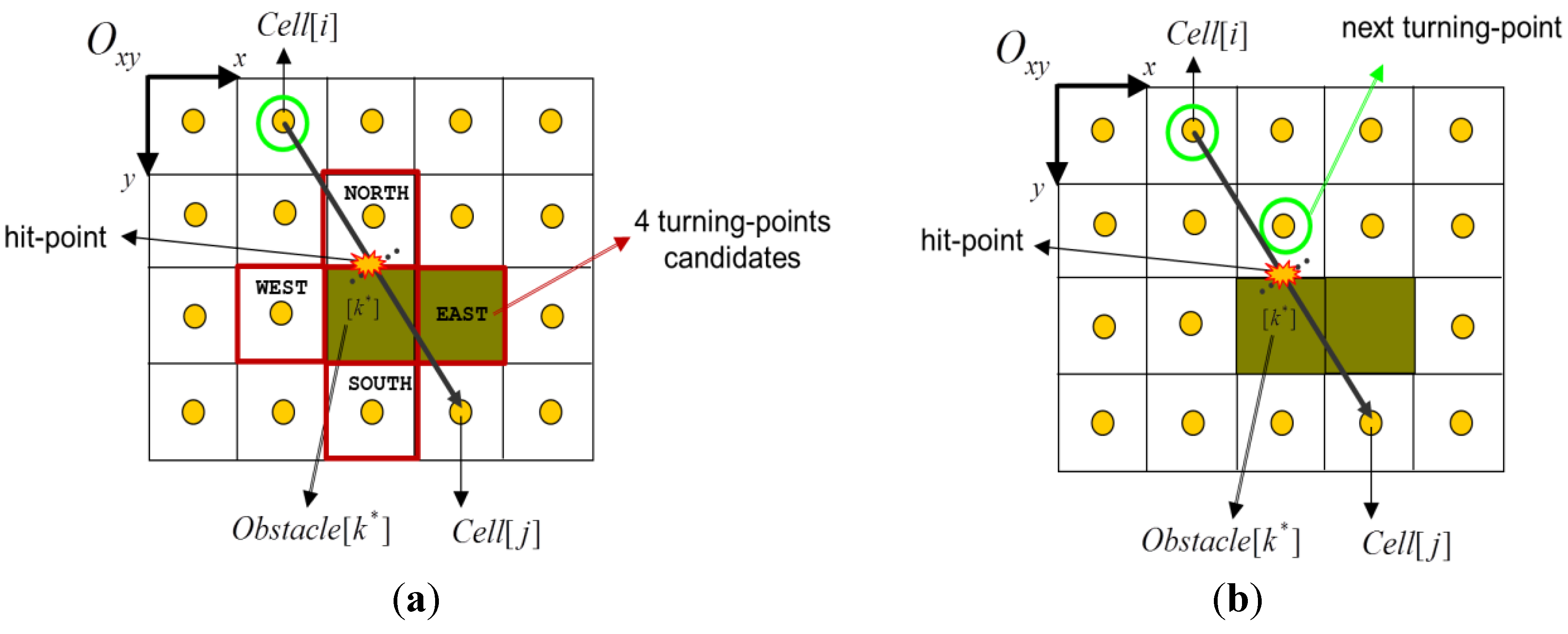
3.2. Choosing the Next Turning-Point

The turning-point selection module, starting from the previously detected collision (see the hit-point in Figure 5), allows the robot to select the proper tile, directly in front of the current obstacle. Following the shortest path-search principles, the turning-point selection module returns the nearest cell from the current position. A new edge representing the next intermediate hop is then appended to the incremental navigation graph.
Given Obstacle[k*], our strategy is to consider the four possible orthogonal tiles (Cell [c]) adjacent to it (EAST, SOUTH, WEST and NORTH in Figure 5). The algorithm evaluates the four candidates checking a list of conditions that asserts the validity of each candidate for the selection:
  • Condition-1: obstacle contour tile;
  • Condition-2: inbound and free tile;
  • Condition-3: not visited and not marked as turning-point;
  • Condition-4: obstacle-free trajectory (from current position).
Figure 5. Selection scheme for the next turning-point: (a) The four possible cardinal candidates;(b) The node returned by the module.
Ijgi 02 00729 g005
Once the invalid cells are removed from the candidate list the algorithm marks the Node[c*] such as d2(i, c*) = minc{d2(i, c*)} by setting its “turningPoint” flag. Node[c*] represents the shortest (intermediate) hop from the current Node[i] towards the target and it is also the cell from which to start surrounding the leading Obstacle[k*]. At this time, the new TurningPoint[c*] is registered into a turning-point list and it is ready to be processed in a new iteration. The instructions to implement this module are presented in Code 2. Depending on the output of the turning-point selection, the HCTNav algorithm switches between one of these three cases:
1)
if no valid candidate is returned, then a dead-end is detected (no new edge is created);
2)
if the new turning-point Node[c*] is different from the current position Node[i], then a new edge is assigned to the path-graph. The pointer Edge[c* ← i] is stored and its weight w is initialized with the straight distance between Cell [i] and Cell [c*] centers;
3)
if the turning-point matches the current position then HCTNav proceeds to surround the obstacle (see next subsection).
Code 2. Turning-point selection pseudo-instructions.
  • Initialize distance(Cell[i], Cell[c*]):= d(i, c*) = ∞
  • Identify the candidates (the four cardinal neighbors of Obstacle[k*] )
  • For every candidate Node[c] in {EAST, SOUTH, WEST, NORTH}:
    • If (Condition-1 = true AND Condition-2 = true AND
      Condition-3 = true AND Condition-4 = true)
      /* Condition-4 calls module for obstacle detection */
      then
      • If d(i, c) < d(i, c*) then
        • update Node[c*]:= Node[c]
        • update d(i, c*):= d(i, c)
  • Return TurningPoint[c*] /* or null, if there are no valid candidates */

3.3. Surrounding Current Obstacle

Starting from the new turning point, HCTNav can determine the two surrounding alternatives to avoid the facing obstacle in the map. Throughout the third module the route is “split” and the navigation graph begins to grow. As result of the obstacle boundary following a list of new turning-points, representing the corner tiles (i.e., 90° path deviations), is returned to be processed later.
To solve the obstacle-surrounding problem, it is necessary to know some information about the tiles’ contour status. That is why we introduced the “contour” flag in the Node[i] properties. During the initialization of the algorithm, the map is preprocessed generating for every contour tile a list of all the adjacent contour neighbors (from now on ContourListi).
This grants that, during execution time, when the obstacle surrounding begins, a turning-point is aware of one or more next-hops from which begin to open the current trajectory in different navigation branches. Hence, starting from the initial ContourListi of TurningPoint[i], the contour neighbors (Node[b]) are visited recursively and added to the list. Same as the filtering technique used in the second module (see Subsection 3.2), the redundancies can be omitted from execution checking similar conditions, except for the third:
  • Condition-3’: not the current position and not in the initial contour list.
Code 3. Obstacles surrounding pseudo-code.
  • Retrieve ContourListi /* contains Node [i] contour neighbors */
  • External loop: While ContourListi is not empty:
    • For every Node [b] in the list
      • If (Condition-1 = true AND Condition-2 = true) then
        • Check corridor from Node [b] to Node [t] /* target */
        • If no obstacles (Obstacle[k*] = null) then
          • Mark Node [b] as turning-point and add to output list
          • Add Edge[b ← i] and Edge[t ← b] to the path-graph
          • Mark Node [b] target-found flag
        • else
          • Retrieve ContourListb /* Node [b] contour neighbors */
          • Go to Internal loop
  • Internal loop: While ContourListb is not empty
    otherwise control goes back to External loop)
    • For every Node [b ' ] in the list
      • If (Condition-2 = true AND Condition-3’ = true) then
        • Check corridor from Node [i] to Node [b ' ]
        • If no obstacles (Obstacle[k*] = null) then
          • Mark previous neighbor Node [b] as turning-point
          • Add Node [b] to output list
          • Add the Edge[b ← i] to the path-graph
      • else
        • Add Node [b ' ] to ContourListi /* neighbor inheritance */
  • Return output list /* or null, if there are no valid corner tiles */
The second condition limits the surrounding redundancies caused by contour neighbors list’s symmetries, whereas the fourth checks that the new Node[b'] can be reached (using the first module of HCTNav to check the corridor). Otherwise, if the way back to the initial position is obstructed, a corner is detected and the correspondent exploration branch ends. Node[b] is marked as turning-point and pushed into the output list, which is composed of all the turning-points discovered during surrounding phase. HCTNav appends this partial list to the main turning-point list and then the algorithm continues to the next iteration. This module consists of two loops: an external one, for processing the current turning-point contour list, and an internal one, for recursively exploring the inherited neighbors. The pseudo-instructions of the third module are shown in Code 3. As it can be seen, in the external loop it is also necessary to check if the way to the target is obstacle free. This is the case of a target-found turning-point (the last hop before the goal).

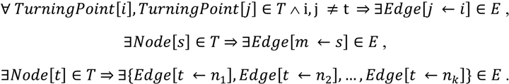
3.4. Building the Final Path

The three main modules described in the previous subsections allow discovering a set of turning-points that is fed back in almost all iterations (except when no valid candidate is available).
Module two returns the next turning-point, whereas module three returns the corner cells discovered during the surrounding. When a turning-point is marked, a new edge representing the hop from current position is constructed and then added to the path-graph, which grows incrementally. The algorithm ends when no more turning-points are available in the main turning-points list, even if the target is not found (this is the case of a path with no solution).
Every turning-point identifies and is pointed by exactly one edge, except for the source (not pointed by any edge) and the target (can be pointed by more than one edge). Hence, it is convenient to reconstruct the path-tree backwards, because the target identifies the exact number of possible paths, thus preventing loops between them. The raw path-graph P := {T, E} is defined by the turning-points list T and the edges set E, such as:
Ijgi 02 00729 i001
To remove the redundancies in the path-graph, due to the generalization of the navigation rules, we developed a post-processing that filters the edges, starting from the target node and proceeding backward until we reach the source node.
As result, a path-tree is available for choosing the shortest path. In Figure 6 a simulation scenario is broken down to better understand HCTNav’s logics and post-processing: given the source position, Node[89] at position (0, 9), and the target point, Node[39] at (8, 3), the raw path-graph is first constructed (Figure 6b); the number of possible paths (two) corresponds exactly to the edges that are pointing to the target node.
Hence, the filtering begins in Node[39], splitting through Edge[39 ← 36] and Edge[39 ← 79]. These two branches correspond to the main trajectory split in TurningPoint[73]. The redundancies that can occur can be classified in two classes: (1) redundant edges, when three turning-points form an unnecessary deviation that can be replaced by one straight edge, and (2) inline edges, when three or more turning-points lie on the same direction.
Figure 6. Full HCTNav case-study: (a) Initial map scenario; (b) Raw path-graph generated; (c) Optimized path-tree; (d) Shortest path returned.
Ijgi 02 00729 g006
Once the optimization process ends (Figure 6c) the path-tree is ready: the “redundant edges” Edge[58 ← 67] and Edge[67 ← 73] have been pruned and replaced by the new Edge[58 ← 73] (thus eliminating the corner in Node[67]). Same as for Edge[74 ← 67] and Edge[67 ← 73], replaced by Edge[74 ← 73], and for Edge[36 ← 60] and Edge[60 ← 58], pruned and replaced by Edge[36 ← 58] The “inline edges” Edge[79 ← 77], Edge[77 ← 75], Edge[75 ← 74] and  Edge[74 ← 73] are normalized (by eliminating TurningPoint[77], TurningPoint[75], TurningPoint[74]) and replaced by the straight Edge[79 ← 73].
A final-path Fk is defined by the ordered sequence of edges that lead from the source node to the target node. During the optimization, for every path Fk, the cumulative distance Wk is also calculated as the sum of all edges in the sequence. When the path-tree is completed, the HCTNav ends (Figure 6d) and returns the shortest path in the optimized tree. The formal definitions for the path-tree structure G* ≔ {T* , E*} are presented in equation (2).
Ijgi 02 00729 i002

4. Experimental Section

In this section a comparison is presented between our algorithm and the two principal families, which represent the state-of-the-art of the deterministic and the reactive approaches (discussed in the introduction of this work). First, a brief overview on our development environment will be given, in order to describe our methodology and testing tools (Subsection 4.1). Second, the experimental results over the map test-suite will be discussed and directly compared to the Dijkstra’s algorithm and its heuristic versions ((Subsection 4.2)). Finally, a qualitative analysis will reveal HCTNav’s improvements with respect to Dijkstra and DistBug’s solutions (Subsection 4.3).

4.1. Test-Bench

Our map test-suite has the characteristics of the model discussed in Section 2: every map is a binary matrix with 15 columns and 10 rows, for a total of 150 tiles. We composed the obstacles profiles of more than 30 maps in order to cover a representative set of topologies, from the more realistic indoor maps to the improbable worst cases maps (Figure 7 shows two maps from our test-suite that will be used in the next subsection for scalability analysis purposes). The test-suite is provided as additional material.
Figure 7. Two examples from the map test-suite, designed by HCTLab team: (a) A “no obstacle” map (map-01); (b) A “labyrinth” map (map-13).
Ijgi 02 00729 g007
The last helped us to stress the algorithm modules and find out potential bottlenecks along the execution flow. We also generated enlarged versions of the maps to better study the scalability of our algorithm and to compare it with Dijkstra’s. Two types of scaling have been defined: (1) topology conservative, by maintaining the aspect ratio of the obstacles profile, and (2) topology repetitive, by replicating the map topology a given number of times. The scaling factors follow the 2-powers pattern (exponential growth): ×2, ×4, ×8, ×16, ×32.

4.1.1. Algorithms Implementation

The code of all the tested algorithms (HCTNav, Dijkstra, A* using Euclidean heuristic) has been implemented in ANSI-C language. The A* implementation follows the guidelines shown in [5]. The A* graph is created using an 8-grid connectivity asserting that diagonal edges avoid collisions. Hence, the generated graph considers the width of the robot when creating the graph. This connectivity was chosen because is the most extended in indoor grid-map-based navigation. Larger connectivity would lead to larger graphs requiring more memory and thus penalizing the comparison. The tie-breaking policy for the A* randomly selects a node from the list of top f-value nodes. Finally, the path obtained by Dijkstra and A* is optimized using the pruning module discussed in Subsection 3.4.
The command-line version of the algorithms allows better studying the dynamic memory usage at run-time, free from graphic libraries and framework’s memory allocations. Further, it allows to launch map-intensive searches, calculating the path for all the possible nodes pairs in all the possible maps of a given set. Each single path-search represents an atomic execution of the given algorithm. To sample the dynamic memory usage we relied on the Valgrind 3.8 (see http://valgrind.org) application and its Massif-msprint tools. The output produced by this memory profiler contains the full record of the RAM allocations, such as mallocs and callocs.

4.2. Simulation Results

In this subsection the experimental data of HCTNav will be presented and directly compared with the Dijkstra family. The four comparison criterions are: (1) dynamic memory usage, (2) scalability over map resizing, (3) execution time, and (4) path length.

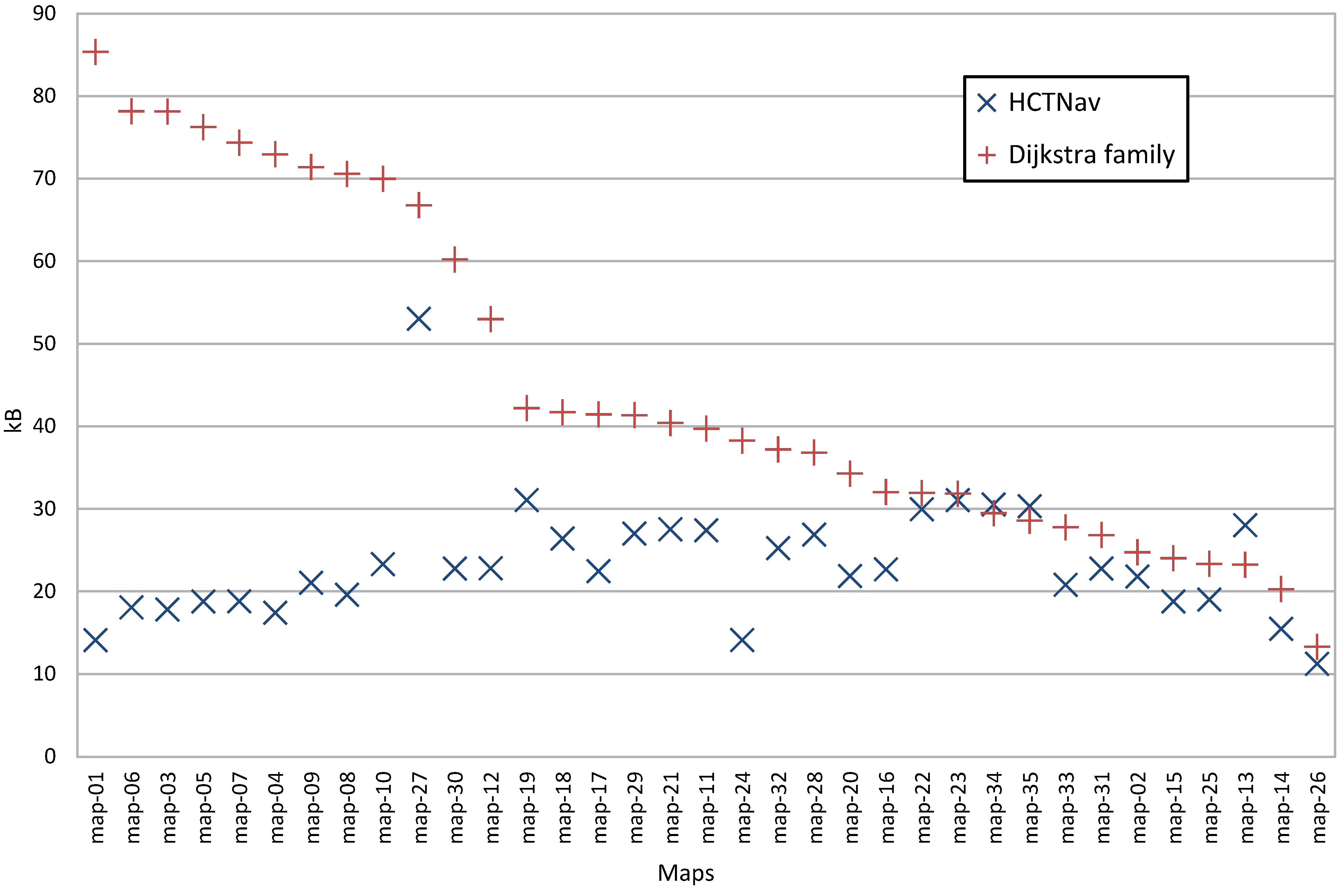
4.2.1. Dynamic Memory Usage

As mentioned in the introduction, HCTNav’s main goal is to minimize memory usage to reduce the design costs of the robot. So, what we are interested for is the “run-time memory peak”, as it represents the minimum upper-bound memory requirement, critical in low-cost systems. The static memory usage is easier to estimate, because it is represented by the executable files and its static data running into the microprocessor. In our own implementation, the Dijkstra’s algorithms occupy about 73.7 kB, whereas HCTNav’s is a 10% greater (about 81.1 kB). For each map in the test suite we measured the dynamic memory required for solving every possible path, capturing the maximum memory allocation sample, or “peak”, in every search (∀i, j : i ≠ j → peak(i, j)).
During the Dijkstra family analysis we found that the dynamic memory usage is identical for all the versions (Dijkstra and Euclidean). This means that the heuristic improvement of the A* family only reduces the overhead problem and enhances execution time but really does not impact the memory usage.
The main component of Dijkstra’s memory allocations grows during initialization and corresponds to the graph building phase and its storing.
In Figure 8 we present a direct comparison between the HCTNav and Dijkstra’s memory requirements at run-time (memory peaks). On the left side of the chart, where maps have a higher rate of free tiles, our algorithm shows a considerable advantage, whereas Dijkstra needs more memory space.
Figure 8. Comparing the dynamic memory “peaks” (HCTNav vs. Dijkstra family). Maps have been ordered considering the result provided by the Dijkstra solution.
Ijgi 02 00729 g008

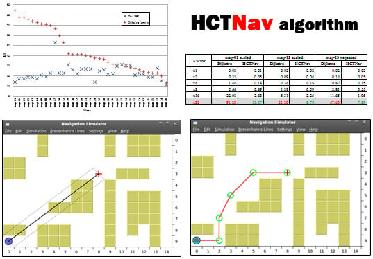
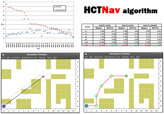
4.2.2. Scalability over Map Resizing

To enforce HCTNav’s benefits in memory usage we have stressed the simulation scenario running rescaled versions of the maps in our set and comparing the response with Dijkstra simulations. The more the graph structures increase in number of cells, the more initial memory space is needed to run the path search in the enlarged map.
The two interesting scenarios we want to discuss here are map-01 (Figure 7a) and map-13 (Figure 7b) as they represent the diametrically opposite map complexity case-studies. The two ways of scaling discussed in Subsection 4.1 are employed. In Table 1 the algorithm results are presented. As it can be seen, the Dijkstra’s algorithms are not as scalable as the HCTNav algorithm: their memory usage is larger in all the scenarios, whereas our solution exhibits a lower growth gradient.
Table 1. Simulation results for the scalability analysis. The dynamic memory peaks are expressed in MB.
Factormap-01 Scaledmap-13 Scaledmap-13 Repeated
DijkstraHCTNavDijkstraHCTNavDijkstraHCTNav
×10.080.010.020.020.020.02
×20.350.050.090.040.140.05
×41.400.180.340.160.670.15
×85.660.691.330.592.810.55
×1622.082.685.312.2511.651.95
×3291.2810.0721.208.7947.407.89

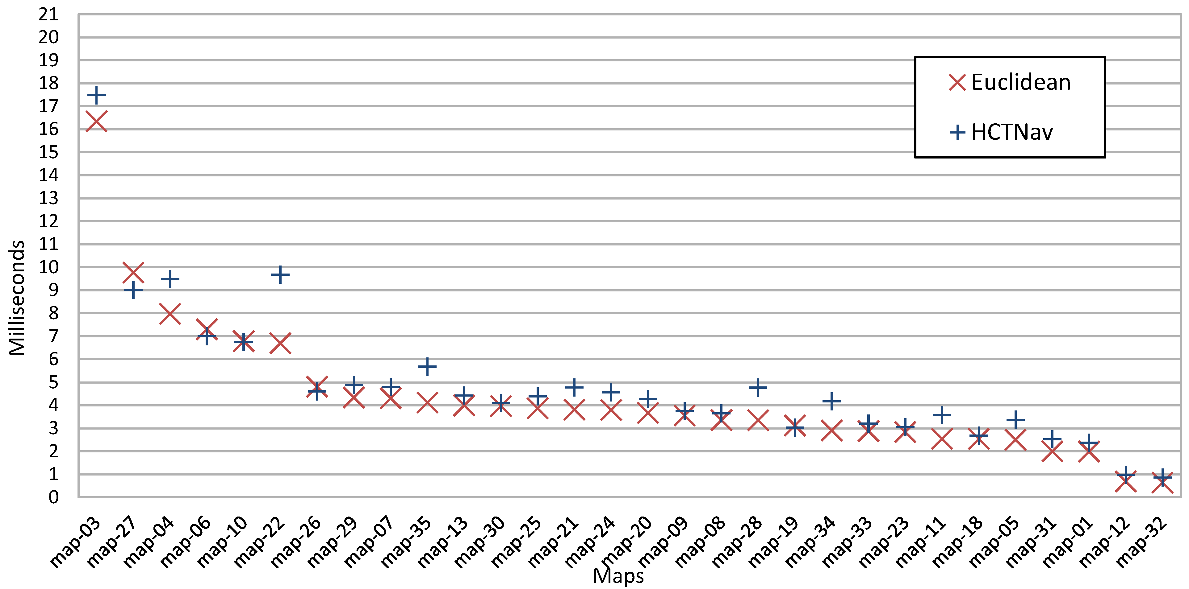
4.2.3. Execution Time Impact

Compared to the easier Dijkstra’s instructions, the execution flow of the HCTNav algorithm can be hard to implement (and to optimize) and adds an undesired degree of complexity to the conventional graph-search algorithms. However, simulation data analysis reveals that HCTNav’s speed performance is acceptable. To measure the execution time we considered the average path search time (i.e., the whole batch job duration divided by the number of available paths). The simulations have been launched on a PC common microprocessor, namely an AMD-64 Turion X2 Dual-core at 2.00 GHz, with 4 GB of RAM and Linux Debian SO (Ubuntu 9.10). The results exhibit that HCTNav’s execution time is in the same order of magnitude of Dijkstra’s (milliseconds).
In complex topologies such as labyrinth-style maps HCTNav loses speed performance, especially if the obstacles’ profile follows a stairway pattern. This is due to the increased switching between obstacle detection and surrounding modules. It is important here to remember that, regarding to the robot’s response time in navigation task (about 30–40 sec of motion in a common scenario), the route planning time is negligible as it does not go beyond the fraction of second.
Figure 9. Execution time comparison (average single-path search). Maps have been ordered considering the result provided by the Euclidean solution (A*).
Ijgi 02 00729 g009
In Figure 9 is presented the execution time comparison between HCTNav and the Dijkstra family over the map test-suite. On the ordinates axis, the average single-path search time is plotted. HCTNav is a bit slower than the A* approach but does not suffer the same speed gap when comparing it with the Dijkstra’s algorithm.

4.2.4. Path Length Comparison

The final comparison between the proposed HCTNav algorithm and the extended Dijkstra and A* solutions evaluates the length of the final path. HCTNav performs a path optimization, as presented in Section 3.4, to reduce the length of the path. The optimization checks if it is possible to move between two non-consecutive nodes shorting the solution. This optimization is also applied to the solution provided by the Dijkstra and A* solutions to make a fair comparison.
Table 2 shows the results of a comparison in a subset of the maps. The difference in granularity of the generated solutions and the application of the optimization algorithm makes a significant percentage of paths to have different path lengths (i.e., up to 22% of the paths in map 11 are different). However, it must be noted that the average difference between path lengths is lower than a third of cell’s length. As stated in Section 2, the length of a cell is the same as the length of the robot. Therefore, this difference is not significant. It must be noted that both the HCTNav and Dijkstra always obtain a solution, although not the same one.
Table 2. Path-length comparison results (mean and variance). The cell’s width is unitary (u =1).
Map NameNumber of Possible PathsPercentage of Different PathsDifference MeanDifference Variance
map-01111750.00%0.000.0
map-02107120.00%0.000.0
map-03101533.20%0.190.6
map-0489114.72%0.250.9
map-0598707.50%0.220.8
map-06101536.30%0.270.1
map-0795915.18%0.300.9
map-0890454.61%0.280.1
map-0989116.06%0.300.1
map-10904512.66%0.300.1
map-11437122.24%0.250.1
map-1264416.27%0.290.6
map-1324859.46%0.290.05

4.3. Qualitative Discussion

4.3.1 HCTNav vs. Dijkstra and A*

Regarding to the Dijkstra family and its heuristic versions (A*), we share the recursive path-graph exploration and part of the data structure that is used during the execution, but with some differences:
  • HCTNav only requires a set of nodes representing the free cells in the binary map, whereas Dijkstra also needs to know all possible edges. This simplification reflects considerable memory saving during run-time, especially when the maps grow in cell number.
  • Edges are composed during the execution and could span multiple nodes; instead, in the common Dijkstra family implementations, used for this comparison, only one-hop edges are evaluated and stored as a preprocessing of the map, due to the exploding cost of storing all the possible edges in the initial graph.
  • In HCTNav we introduced an obstacle control strategy to find the intermediate transit nodes (turning-points) from which to begin to surround obstacles. Dijkstra simply does not consider obstructions as they are implicitly removed at the construction of the initial graph.
  • The difference between the path lengths between the HCTNav and the Dijkstra is lower than a third of a cell. Considering that it is also a third of the size of the robot, it is not significant.
In Figure 10a direct comparison of HCTNav and Dijkstra family is presented in another case-study scenario (map-11). In these simulations we are focusing on the “overhead” rate, i.e., the map’s portion that is explored even if it is not useful to reach the target. This factor is critical because it impacts directly the path-search performance. As it can be seen, HCTNav approximates the A* overhead (Figure 10d), which is smaller than Dijkstra due to the proper next-hop choice.
Figure 10. Qualitative analysis in map-11: (a) Initial trajectory scenario; (b) HCTNav solution and overhead; (c) Dijkstra’s algorithm; (d) A* algorithm.
Ijgi 02 00729 g010

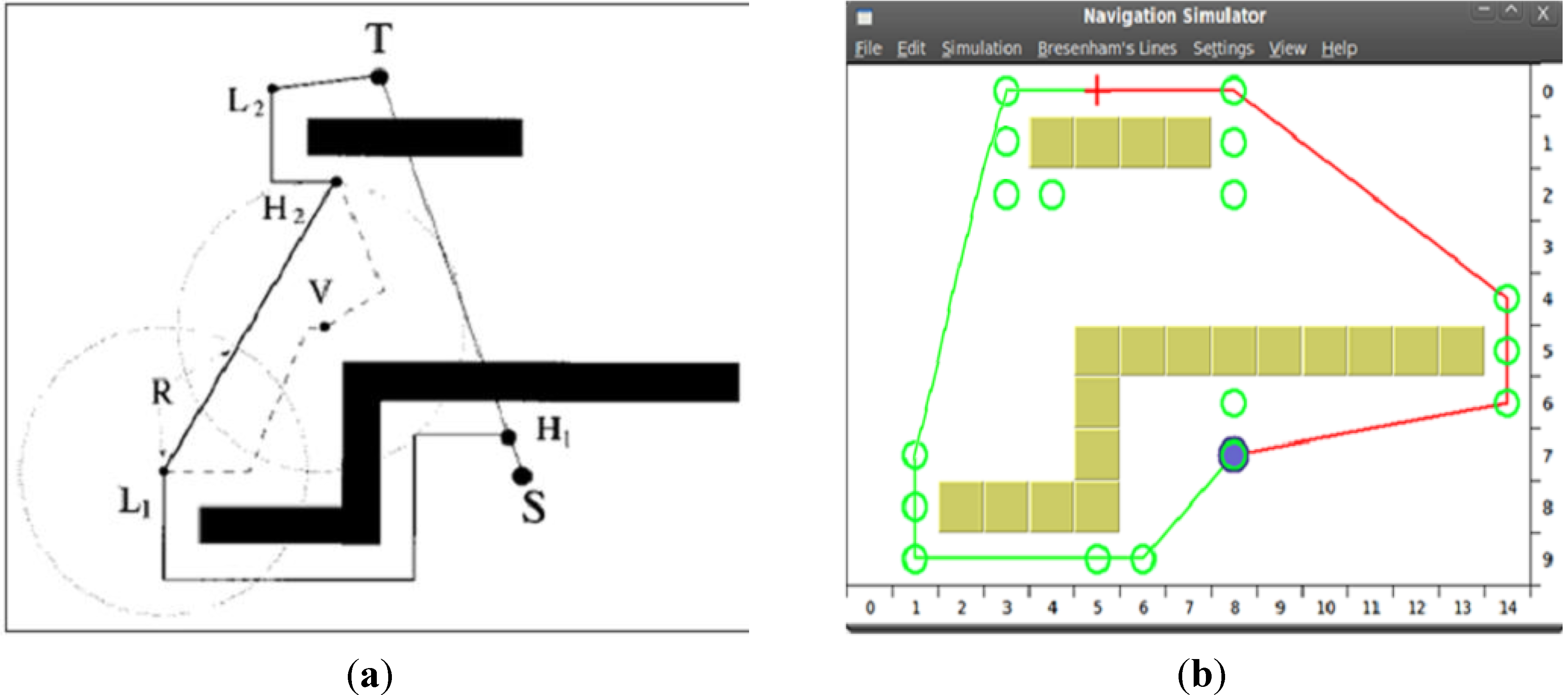
4.3.2. HCTNav vs. DistBug

With respect to the Bugs family, the HCTNav approach is quite different: the Bugs are based on the complete lack of map information, whereas HCTNav has an a priori knowledge of the map model; in consequence of that, the HCTNav navigation concept is opposite of Bugs family’s (graph exploration vs. sensory-based motion).
Nevertheless, we have found that our navigation rules are similar to the DistBug’s operative modes (motion towards the target and obstacle-boundary following). This is due to the fact that both algorithms are inspired on human-based intuitive strategy to reach to a destination avoiding obstacles.
The same criterion is valid for both an unknown environment and a map-planning scenario. The choice of which strategy to implement is bound to the trade-off between robot design costs and algorithm’s complexity. The DistBug logical layer is simpler than the HCTNav’s but also the cost of sensor layer of the DistBug robot is greater than the HCTNav’s.
In Figure 11 we have reproduced a simulation scenario from the Kamon and Rivlin’s work [13]. Although it represents only a theoretical result for the DistBug algorithm (not simulated), the map fits into our simulation model, i.e., a grid with linear obstacles profile. The robot’s width is taken into account in DistBug too, by setting a proper security range in the proximity sensor array. A clear benefit of pre-processing the robot motion in a known indoor environment is that the trajectory found is, in general, shorter thus extending on-board batteries lifetime in a long task scenario. As expected, our navigation path-tree includes the DistBug solution (left branch in Figure 11b): we can observe that even H1 and H2 points (Figure 11a) are reflected as HCTNav’s turning-points. But also, HCTNav finds other possible solutions, which are also evaluated (which are also shorter). HCTNav also includes a pruning module (see Subsection 3.4), taking advantage of map information, removes the unnecessary corners by replacing them with new edges to reduce the cumulative final distance. The best solution here is represented by the path on the right in Figure 11b.
Figure 11. Navigation results of DistBug and HCTNav. HCTNav would find a shortest path to the right of the obstacles (red line). (a) DistBug’s theoretical solution; (b) HCTNav’s solution.
Ijgi 02 00729 g011

5. Conclusions

This paper has described a path-planning algorithm for low-cost robots navigating in indoor environments. Starting from analyzing the pros and cons of the two most popular approaches in navigation problem: the deterministic and the reactive; we proposed a hybrid solution, the HCTNav.
Our initial goal was to minimize the hardware’s requirements of the robot’s navigation layer. In fact, in the deterministic approach, referenced by the Dijkstra family algorithms, a big amount of RAM memory is needed to store the graph structure; in the reactive approach, referenced by the Bug family algorithms, the major cost is represented by the intensive sensor sampling and the related control hardware. HCTNav’s concept is to combine the shortest-path search principles of the deterministic approach with the obstacle detection and avoidance techniques of the reactive one.
To reduce the dynamic memory upper-bound limit at runtime, we designed the data structure of the algorithm to eliminate the edge set from the initial graph. Further, we were able to reduce the sensors layer requirements by implementing the obstacle boundary-following as pure software, instead of sampling the environment with proximity sensors. The main HCTNav requirement is that the robot must be aware of the map’s topology a priori. Our map’s model is a binary matrix representing the occupancy map-grid with the cell’s status (free or occupied). The new edges in the graph are discovered dynamically, by scanning the desired trajectory with the Bresenham’s line algorithm. When a potential collision is detected, a turning-point adjacent to the leading obstacle is marked as the next hop. Starting from this new intermediate point, the initial trajectory is split into different navigation branches allowing the robot to surround obstacles by following their boundaries. Hence, HCTNav generates a navigation graph that leads from the initial position to the target point. To obtain the shortest path from the obtained solutions, a post-optimization strategy eliminates the redundant edges, due to inline turning-points and unnecessary corners, by replacing them with normalized edges.
By keeping in mind that map-grids in real scenarios can hold thousands of cells, we focused our efforts on making the algorithm as scalable as possible. To measure the HCTNav’s performances we developed our own test-bench, relying on the Valgrind memory profiler and on a custom map test-suite with different topologies. As seen, the map topology and the obstacle profile represent a critical factor in the performance of any navigation algorithm. HCTNav takes advantage from maps with a low obstacle presence, whereas Dijkstra family is penalized in memory usage when the ratio between free tiles and obstacles is high.
The simulations have proved that our algorithm needs less memory space than the Dijkstra’s algorithm or its heuristic versions, especially when the map granularity grows. For example, in a 32× rescaled map scenario (more than 150,000 cells), the HCTNav’s memory peak is nine times lower than Dijkstra family’s. Further, the experimental results reveal that Dijkstra and the A* algorithms exhibit the same memory usage. This means that the A* solution only improves the Dijkstra overhead and execution time but do not reduce the memory usage, whereas HCTNav is more suitable for implementing on a low-cost robot microprocessor with limited resources. The execution time is still acceptable as it keeps in the same order of magnitude of Dijkstra. The differences between path lengths are not significant in the low percentage of paths that this difference has arisen. Regarding to the comparison with the Bug family, HCTNav reduces both the final-path length, thus granting longer battery lifetime; and the sensory layer complexity, thus reducing the hardware costs.

Acknowledgements

This work has been partially supported by the Spanish “Ministerio de Ciencia e Innovación”, under project TEC2009-09871.

Conflict of Interest

The authors declare no conflict of interest.

References

  1. Fu, L.; Sun, D.; Rilett, L.R. Heuristic shortest path algorithms for transportation applications: State of the art. Comput. Oper. Res. 2006, 33, 3324–3343. [Google Scholar] [CrossRef]
  2. Antich, J.; Ortiz, A.; Minguez, J. A Bug-Inspired Algorithm for Efficient Anytime Path Planning. In Proceedings of the IEEE/RSJ International Conference on Intelligent Robots and Systems, St. Louis, MO, USA, 10–15 October 2009; pp. 5407–5413.
  3. Cormen, T.H.; Leiserson, C.E.; Rivest, R.L.; Stein, C. Dijkstra’s Algorithm. In Introduction to Algorithms, 2nd ed.; MIT Press: Cambridge, MA, USA, 2001; pp. 595–601. [Google Scholar]
  4. Idris, M.; Bakar, S.; Tamil, E.; Razak, Z.; Noor, N. High-Speed Shortest Path Co-Processor Design. In Proceedings of Third Asia International Conference on Modelling & Simulation, Bali, Indonesia, 25–29 May 2009; pp. 626–631.
  5. Cain, T. Practical Optimizations for A* Path Generation. In AI Game Programming Wisdom, 2nd ed.; Charles River Editors: Boston, MA, USA, 2003; pp. 146–152. [Google Scholar]
  6. Grant, K.; Mould, D. Combining Heuristic and Landmark Search for Path Planning. In Proceedings of the Confereunce on Futre Play: Research, Play, Share, Toronto, ON, Canada, 3–5 November 2008; pp. 9–16.
  7. Goto, T.; Kosaka, T.; Noborio, H. On the Heuristics of A* or A Algorithm in ITS and Robot Path Planning. In Proceedings of IEEE/RSJ International Conference on Intelligent Robot and Systems, Las Vegas, NV, USA, 27–31 October 2003; pp. 1159–1166.
  8. Bollobas, B. Modern Graph Theory; Springer: Heidelberg, Germany, 1998; pp. 252–259. [Google Scholar]
  9. Selamat, A.; Zolfpour-Arokhlo, M.; Hashim, S.Z. A Fast Path Planning Algorithm for Route Guidance System. In Proceedings of IEEE International Conference on Systems, Man and Cybernetics, Anchorage, AK, USA, 9–12 October 2011; pp. 2773–2778.
  10. Langerwisch, M.; Wagner, B. Dynamic Path Planning for Coordinated Motion of multiple Mobile Robots. In Proceedings of IEEE International Conference on Intelligent Transportation Systems, Washington, DC, USA, 5–7 October 2011; pp. 1989–1994.
  11. Zhou, J.; Lin, H. A Self-Localization and Path Planning Technique for Mobile Robot Navigation. In Proceedings of the Intelligent Control and Automation (WCICA), Taipei, China, 21–25 June 2011; pp. 694–699.
  12. Abdul-Jabbar, J.M.; Alwan, M.A.; Al-ebadi, M. A new hardware architecture for parallel shortest path searching processor based-on FPGA technology. Int. J. Electron. Comput. Sci. Eng. 2012, 1, 2572–2582. [Google Scholar]
  13. Jiang, Z.; Wu, J. On Achieving the Shortest-Path Routing in 2-D Meshes. In Proceedings of the Parallel and Distributed Processing Symposium, Long Beach, CA, USA, 26–30 March 2007; pp. 26–30.
  14. Lumelsky, V.J.; Stepanov, A. Path-planning strategies for a point mobile automaton moving amidst obstacles of arbitrary shape. Algorithmica 1987, 2, 403–430. [Google Scholar] [CrossRef]
  15. Lumelsky, V.J.; Skewis, T. Incorporating range sensing in the robot navigation function. IEEE Trans. Syst. Man Cybern. 1990, 2, 1058–1068. [Google Scholar] [CrossRef]
  16. Kamon, I.; Rivlin, E. Sensory-based motion planning with global proofs. IEEE Trans. Robot. Autom. 1997, 13, 814–822. [Google Scholar] [CrossRef]
  17. Knudson, M.; Tumer, K. Adaptive navigation for autonomous robots. Auton. Robots 2011, 59, 410–420. [Google Scholar] [CrossRef]
  18. Sharef, S.M.; Sa’id, W.K.; Khoshaba, F.S. A Rule-Based System for Trajectory Planning of an Indoor Mobile Robot. In Proceedings of the International Multi-Conference on Systems Signals and Devices, Amman, Jordan, 27–30 June 2010; pp. 1–7.
  19. Yu, N.; Ma, C. Mobile Robot Map Building Based on Cellular Automata. In Proceedings of the Pacific-Asia Conference on Circuits, Communications and System, Wuhan, China, 17–18 July 2011; pp. 1–4.
  20. Gonzalez-Arjona, D.; Sanchez, A.; de Castro, A.; Garrido, J. Occupancy-Grid Indoor Mapping Using FPGA-Based Mobile Robots. In Proceedings of the Conference on Design of Circuits and Integrated Systems, Albufeira, Portugal, 16–18 November 2011; pp. 345–350.
  21. Buckland, M. Programming Game AI by Example, 1st ed.; Wordware Publishing: Plano, TX, USA, 2005; pp. 193–248. [Google Scholar]
  22. Bresenham, J.E. Algorithm for computer control of a digital plotter. IBM Syst. J. 1965, 4, 25–30. [Google Scholar] [CrossRef]

