Article

Conflation Optimized by Least Squares to Maintain Geographic Shapes

1
COGIT-IGN, 73 avenue de Paris, 94165 Saint-Mandé, France
2
IGN, 73 avenue de Paris, 94165 Saint-Mandé, France
*
Author to whom correspondence should be addressed.
ISPRS Int. J. Geo-Inf. 2013, 2(3), 621-644; https://doi.org/10.3390/ijgi2030621
Submission received: 5 May 2013 / Revised: 21 June 2013 / Accepted: 24 June 2013 / Published: 3 July 2013

Abstract

:
Recent technologies allowed a major growth of geographical datasets with different levels of detail, different point of views, and different specifications, but on the same geographical extent. These datasets need to be integrated in order to benefit from their diversity. Conflation is one of the solutions to provide integration. Conflation aims at combining data that represent same entities from several datasets, into a richer new dataset. This paper proposes a framework that provides a geometrical conflation that preserves the characteristic shapes of geographic data. The framework is based on least squares adjustment, inspired from least squares based generalization techniques. It does not require very precise pre-matching, which is interesting as automatic matching remains a challenging task. Several constraints are proposed to preserve different kind of shape and relations between features, while conflating data. The framework is applied to a real land use parcels conflation problem with excellent results. The least squares based conflation is evaluated, notably with comparisons with existing techniques like rubber sheeting. The paper also describes how the framework can be extended to other geometrical optimization problems.

1. Introduction

Together with the developments of GI technologies and Web 2.0, the number of available geographical datasets has increased tremendously in the past years. Among this diversity, data quality, level of detail, modeling choices, and content may greatly differ. In order to enable or expand complex spatial analyses, trying to integrate datasets from different sources can be very attractive but quite difficult. Two options are possible to integrate data from different sources, multi-representation databases, and conflation. Multi-representation databases allow us to model real world objects with different representations according to scale or point of view. The integration in such a database implies to match the representations from the different sources [1]. The paper only considers the second option, the conflation of the datasets into a richer one.
Conflation aims at combining data that represent the same real world entities, from several datasets, into a richer new dataset that contains information that cannot be obtained from any of the single datasets alone [2]. The more datasets have different representations or levels of detail, the more difficult conflation is. For instance, conflation is required if a National Mapping Agency seeks to integrate Volunteered Geographic Information (VGI) [3] like OpenStreetMap data, that is often captured with less accurate techniques, either to enrich its datasets with VGI or to improve geometrical consistency between datasets. Conflation can generally be divided into three steps: data matching, geometry deformations and attribute merging. Each step is a challenging task, but the paper only focuses on the geometry deformation task, once data matching has succeeded. The issue of the geometry deformation task is generally to snap the less accurate data sources geometries to the most accurate data sources geometries. The case with similar accuracy datasets is not tackled by the paper but briefly discussed in Section 4.5.
The shape of geographic data conveys essential implicit information for analysis (e.g., curvature, sharp angles). Conflation deformations may transform the initial shapes and convey misleading information. For instance, a straight road should not become curved and building should not lose their right angles. Added to that, spatial relations, like the relative position of a building to a dead-end road, should not be destroyed by the conflation process. As a consequence, finding a deformation model that takes shape and spatial relations into account, when absorbing deformations, is key topic for the improvement of conflation techniques. The paper tries to tackle this key topic by proposing a deformation model that balances snapping considerations with preserving shape and spatial relations considerations, thanks to least squares optimization.
The second part of the paper describes related work on conflation. The third part proposes a model to conflate data by least squares optimization in order to maintain the initial shape of data. The fourth part presents experiments on a use case with land use data. Part five draws some conclusions and describes future work.

2. Related Work

Conflating data requires, first, to match data that reflects the same real world entity, then to merge their geometry and their attribute data. Although the paper does not focus on data matching, this section describes previous work on the automatic matching of geographic data, as it is a necessary pre-condition of the presented geometry fusion method.
First, all data matching methods rely on some kind of similarity measures to figure out if the features represent the same real world entity [4]. Similarity measures for data matching can be classified into three categories: geometry, attribute, and topology [5]. Geometry measures that compare two linear shapes [6], or polygonal shapes [7,8], can be used to evaluate the difference between the conflated and the original geometries (Figure 1). Such comparison allows the quantification of the distortions of conflated polygonal features.
Figure 1. The surface distance to assess two polygons similarity, the ratio between the areas of the grey surfaces (the intersection of polygons A and B and their union).
Ijgi 02 00621 g001
Data matching can be achieved by theme specific methods. For instance, as coastlines are very sinuous, similarity, and one-to-one matching, can be achieved using Fréchet distance [9]. In networks, like road or river networks, topology, i.e., how network elements are connected to each other, allows matching networks with quite different level of details [10].
Although geographic data can be very specific from theme to theme, efficient generic matching methods have been proposed in the literature. The method proposed by Walter and Fritsch [5] examines the similarity of features in each pair, and statistical considerations globally determine the best set of matching pairs. The data matching process described by Samal et al. [11] proposes to use a large number of similarity measures and averages the similarity scores to find the best match. As data matching relies on several different criteria, multiple criteria analysis techniques can be applied to decide if features can be matched [12]: geometry, attribute, and topology criteria can be mixed to match features with a very high accuracy. If the matches are considered globally, finding a matching that maximizes the similarities can also be considered as an optimization problem [13].
The problem of geometry transformation, or snapping the least precise geometries on the most precise ones, has already been tackled by a few researchers. First, geometry fusion can be achieved by creating a new geometry that replaces the ones of the matched features with an average position [14]. It is a valuable method when levels of detail are similar and when no dataset is more precise than the others.
Although it was proposed for frontier connection purposes, rubber sheeting can be applied to conflation to snap the less precise geometries on the most precise ones [15]. This rubber sheeting principle has been extended to produce a deformation vector field from the previously matched features [16,17,18]: each control point computed from matching contributes inversely proportionately to the distance to the point that is to be deformed (Figure 2). Haunert [16,17] shows that this method is very interesting, but its drawback is that shapes can be quite deformed and lose their expressivity: straight roads may become curved for instance. Furthermore, Gruendig et al. proposes an alternative method that attempts to take building rectangularity into account during conflation based on least squares adjustment [19]. The details of the adjustment method are not given but it relies on a full matching of geometry nodes and on positional accuracy information, which limits its usability (e.g., if one layer is not present in both datasets, its features cannot be matched). Moreover, few shape characteristics are taken into account.
Figure 2. The principles of rubber sheeting conflation (a) the black geometries match with the green ones (b) a vector field is computed to make the black features fit into green feature’s geometry.
Ijgi 02 00621 g002
Finally, it is possible to model conflation in its entirety with a global framework, as Cobb et al. [20] propose a global method that tackles all three steps. First, data matching is achieved by a multiple criteria rules-based system. Then, attribute fusion is achieved using quality metadata. Finally, there is a two-step geometry fusion: first, a mesh-based rubber sheeting is triggered, and then an interpolation guided by precision information is carried out. Adams et al. propose a generic framework [2], where conflation is assimilated as similarity plus error estimation: similarity is the aggregation of spatial and semantic similarity and the error estimation is the difference between the initial features and the conflated ones (the error may apply to both geometry and semantics).
Nevertheless, as the issue of this paper is a framework for geometry fusion during conflation, which does not include the other steps of conflation, it focuses on the development of an alternative to rubber sheeting that allows preserving the shapes of conflated features, whether the features are man-made with straight shapes and right angles, or natural with smooth curved shapes.

3. Conflation by Least Squares Optimization

The proposed conflation model was inspired by map generalization models that are briefly presented in the first section. The second section describes the principles of the least squares based conflation model, then details the constraints to maintain shape, the ones to conflate data, and finally explains how additional data can be propagated.

3.1. Least Squares Based Map Generalization

Least squares adjustment is, among others, a mathematical method to solve linear equations systems when the systems have more equations than unknowns, and are therefore unsolvable exactly. The approximate least squares solution for the linear system minimizes the sum of squared residuals (the difference from the exact solution for each equation) [21]. A linear system can be expressed with matrices, using the Jacobean matrix A (Equation (1)) and its solution can be expressed with a residual vector v (Equation (1)).
Ijgi 02 00621 i001
If we add a weighting matrix P that conveys the relative importance of each equation (e.g., it is more important to be close to solution for equation i than for equation j), the least squares adjustment finds a solution that minimizes:
Ijgi 02 00621 i002
This solution is obtained by matrix inversion and is the following:
Ijgi 02 00621 i003
The specifications that make a generalized map legible (e.g., the minimum size of symbols, the minimum distance between close symbols, etc.) can favorably be expressed with constraints [22]. “Buildings should be 0.1 map mm apart” is an example of constraint to specify a map generalization process and most of existing automatic generalization processes are guided by such constraints, including the ones based on least squares. In order to make legible but close to ground truth maps, rival constraints have to be defined: on the one hand, constraints to have simplified and bigger features and on the other hand, constraints to maintain the initial shape or position.
Two least squares based generalization processes were proposed independently and simultaneously some years ago [23,24]: both translate the constraints into linear equations, similar to (Equation (1)), and find an optimal solution by the least squares adjustment. The weights of (Equation (2)) correspond to the constraints relative importance (some constraints are more important to satisfy than others). The unknowns of the equations are the coordinate’s difference for each vertex of the objects geometries (Figure 3). As a consequence, there are much more linear equations than unknowns in the system and the least squares method provides an optimal solution to the position of each vertex according to the constraints.
Figure 3. How to translate generalization into a linear equation system.
Ijgi 02 00621 g003
Sester and Harrie proposed a small set of constraints that can be translated into linear equations on the vertices [23,24]. For instance, constraints to maintain the initial position or to ensure a minimal distance between buildings were proposed. Most of these constraints could be used in a conflation problem in order to preserve the shape and position of conflated features.

3.2. Least Squares Applied to Conflation

The proposed shape preserving conflation framework is based on the least squares generalization model presented in the previous section. The next section describes its principles; then, constraints to maintain shape, to conflate data and to maintain data consistency are presented; finally, additional propagation mechanisms are proposed.

3.2.1. Principles

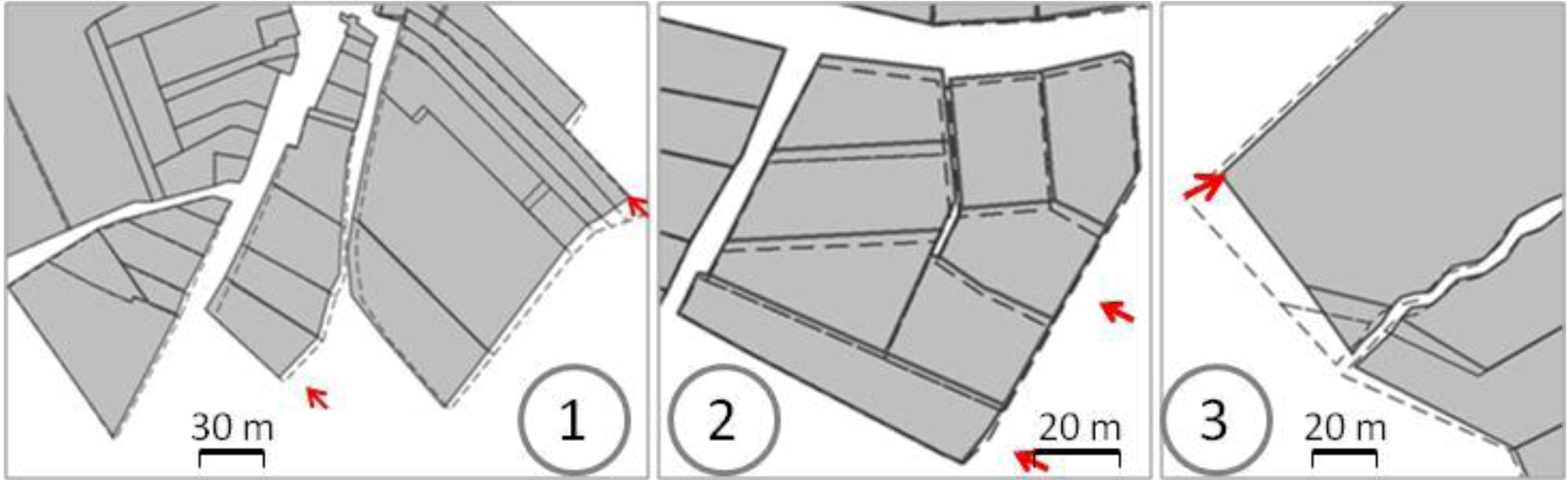
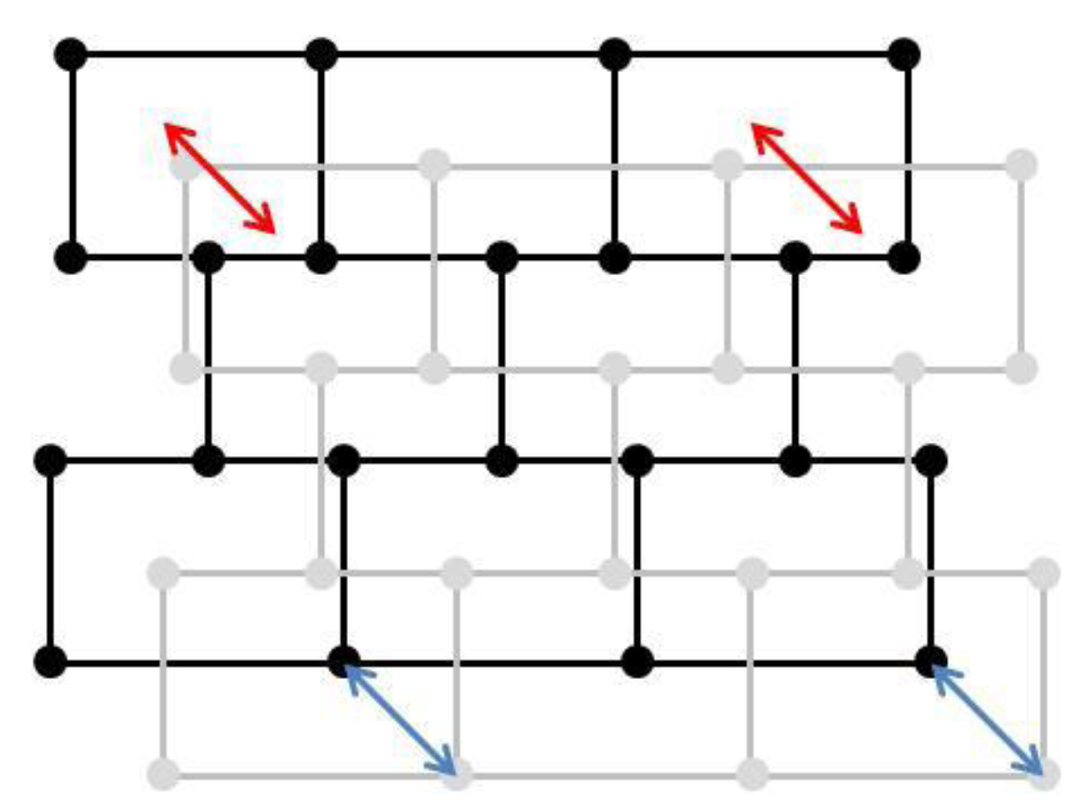
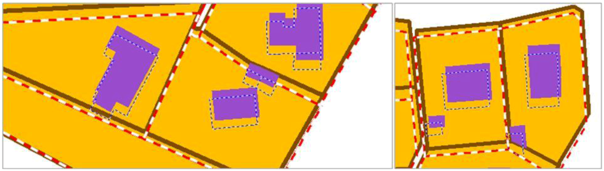
The proposed framework requires a major hypothesis on input data: the datasets to conflate have to be matched, at least minimally. A full feature-to-feature matching is not necessary (Figure 4). The matching result may be either matched vertices or matched features, like in Figure 4, but at least one feature or one vertex has to be matched. It is the only requirement for the matching: the framework is able to conflate dataset with one matching or with half of the features matched. Displacement vectors are extracted from the matching, which will guide the least squares conflation: the vectors are computed from points of the matched features belonging to the least precise dataset to points of the corresponding feature in the most precise dataset. If the matched features are structurally different (e.g., not the same level of detail and thus, a different number of vertices), it is not a problem as a displacement vector can be extracted from the centroid, for instance.
Figure 4. Two sets of polygonal data to be conflated: two feature-to-feature matchings (red arrows) and two vertex-to-vertex matchings (blue arrows).
Ijgi 02 00621 g004
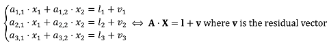
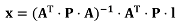
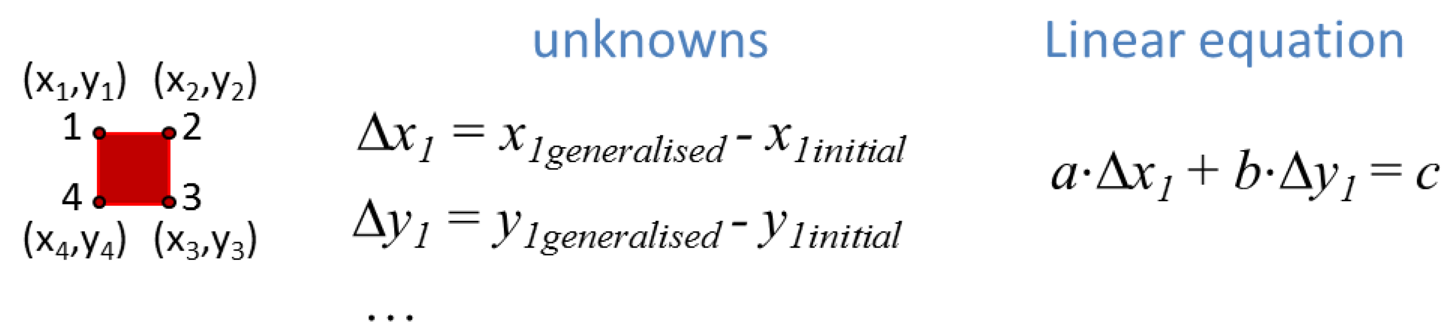
The principles of the least squares shape preserving conflation model takes the generalization model up. The unknowns in the linear equation system are the coordinate displacements ∆x and ∆y (including points that were not matched). The unknowns are not the difference between points before and after generalization anymore, but the difference before and after conflation. The equations are translations of constraints on the features to be conflated: a constraint on a feature is translated by one (or more) equation for every point of the feature geometry. Constraints introduced to conflate data are balanced by constraints to preserve the initial shape which leads to an over constrained linear system. As the main goal of the conflation model is to merge geometries, the constraints that control conflation are weighted more than the constraints that preserve shapes. Indeed, weight setting is a key task in this least squares framework [25]. In order to avoid overloading the equation system, some features can be excluded from the least squares and be conflated thanks to propagation mechanisms derived from map generalization techniques [26]. Finally, the shape preserving conflation model provides assessment of the deformations carried out to conflate data, derived from residual vector v, which gives a direct value for the geometrical error estimation of Adams et al. [2].

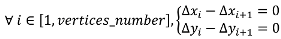
3.2.2. Constraints to Preserve Shape

In order to preserve the shapes of the conflated objects, specific constraints can apply to them, depending on the feature type: for instance, stiffness constraints can apply to buildings or urban land use parcels and curvature constraints can apply to rivers or natural land use parcels. However, a constraint is common to all feature types to avoid over displacements that could lead to horizontal positioning errors: the initial position of the conflated features should be preserved. It corresponds to the movement constraint described by Harrie [23] and it is translated into two simple equations:
Ijgi 02 00621 i004
As it is a very restrictive constraint, it should be very slightly weighted to allow some movements in the least squares solutions. For instance, the weight put in the P matrix lines corresponding to this constraint is 1 in our experiments while other constraints (e.g., the conflation constraint described in Section 3.2.3) have a weight of 20.
In order to preserve the shape of features that should only be translated and/or rotated, the stiffness constraint from Harrie [23] constrains the position of successive vertices (Equation (5)).
Ijgi 02 00621 i005
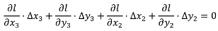
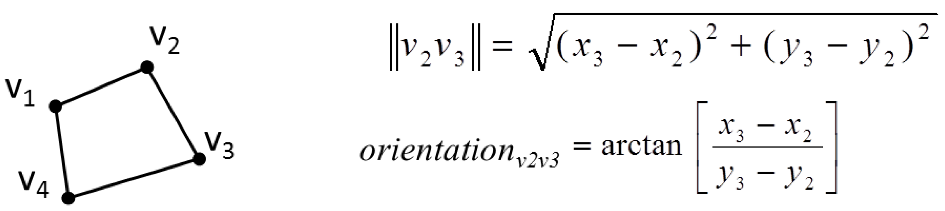
Alternative preserving constraints are possible for stiff objects that are allowed to be distorted a little more than with the stiffness constraint: a side orientation constraint and a segment length constraint [24] (Figure 5). Both equations are nonlinear but can be linearized by derivation, as the unknowns are here ∆x and ∆y. Thus, the preservation of length l of the segment |v2, v3| would be the linear Equation (6). The same linearization can be applied to the side orientation constraint.
Figure 5. Nonlinear equations for segment length and orientation in a stiff feature.
Ijgi 02 00621 g005
Ijgi 02 00621 i006
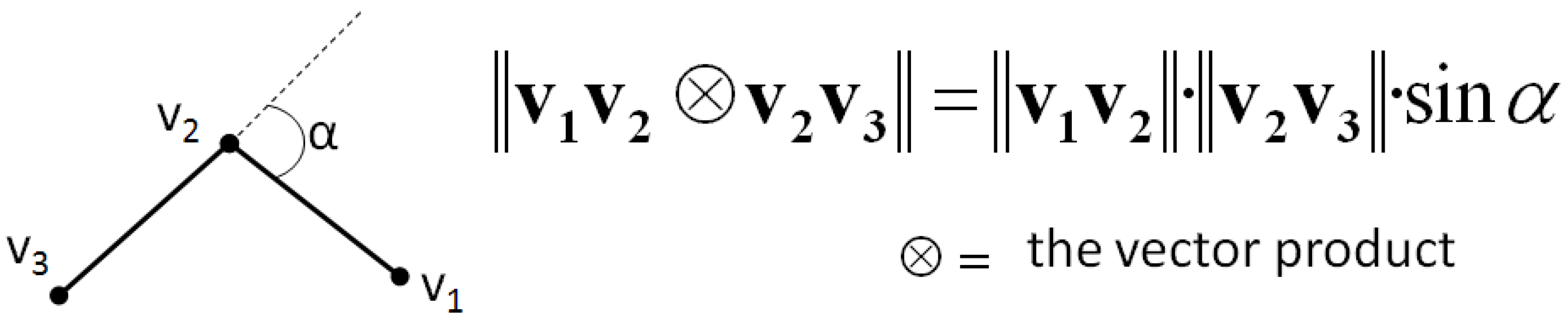
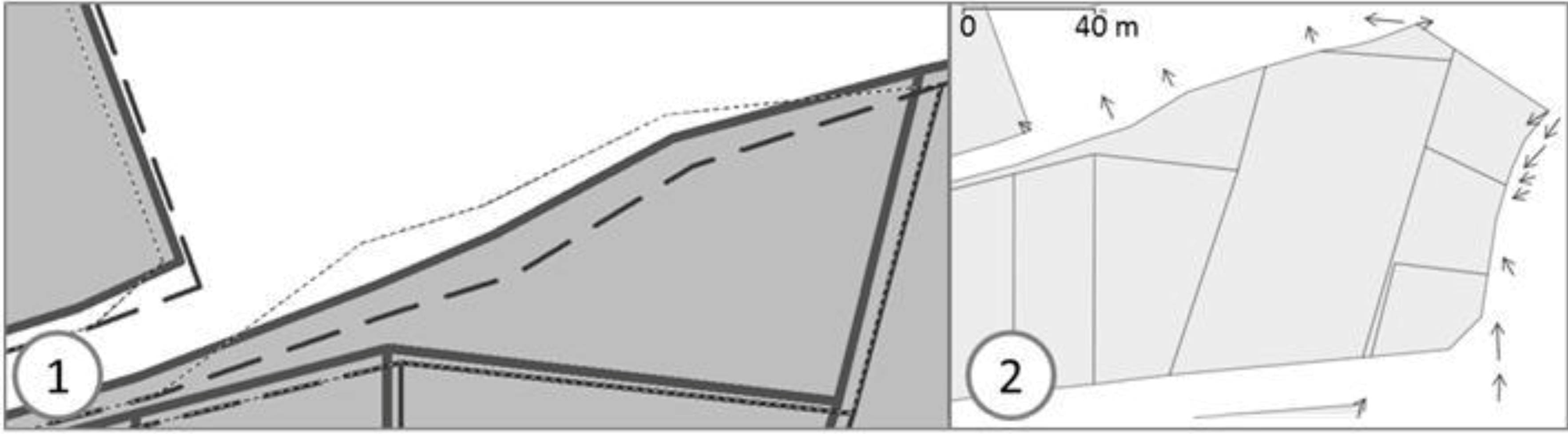
The previous shape preservation constraints are mostly dedicated to stiff (or man-made) features like buildings, streets, or parcels. But considering features whose shape was crafted by nature like rivers, forests, mountain roads, or lakes, requires the definition of other constraints. We propose to use the curvature constraint introduced by Harrie [23] that forces the preservation of the curvature between successive line segments. The problem of curvature preservation is transformed into a simpler problem, the preservation of the angle α between two successive line segments, which is linearized using the vector product definition (Figure 6). The computation of the linear equation from the vector product is detailed by Harrie [23].
Figure 6. Expression of the curvature preservation constraint.
Ijgi 02 00621 g006

3.2.3. Constraints to Conflate Data

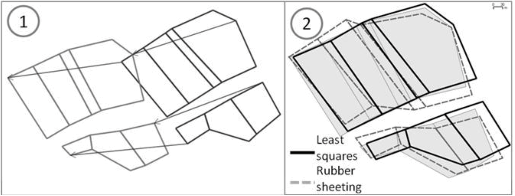
To balance the constraints to maintain shape, it is necessary to introduce constraints that force conflation. We compute such constraints based on matches of features. Our least squares conflation framework requires these matches as input. Three kind of conflation constraints are proposed in the framework from very local action to propagation actions close to the rubber sheeting approach. For each one, the cases where it should be used are briefly discussed.
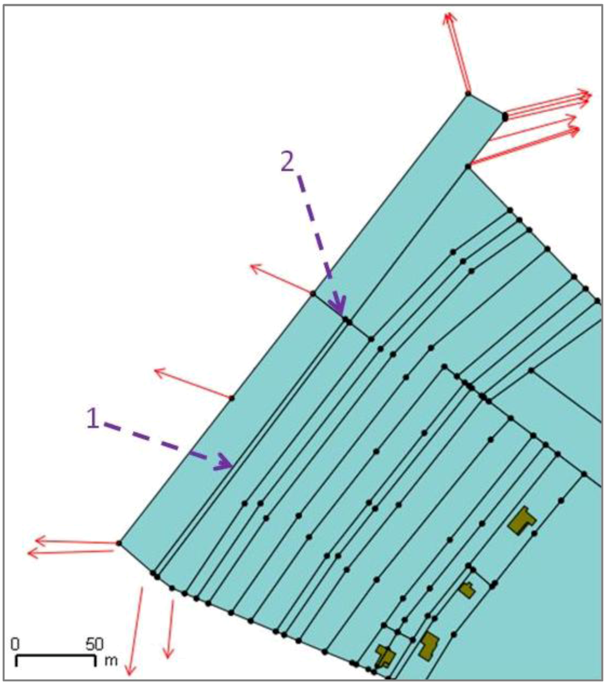
All constraints rely on the computing of displacement vectors from the features matched in the conflated datasets. For each matched feature, the feature matching is transformed into vertex matching: the vertices in the less detailed dataset are matched to vertices of the matched feature in the most detailed dataset (Figure 7). Displacement vectors are computed for each matched vertex from the least detailed dataset to the most detailed one: the vectors represent the displacement the vertices should do, to conflate the geometries.
Figure 7. Computing vector displacement from the partial matching of features (the textured features are matched).
Ijgi 02 00621 g007
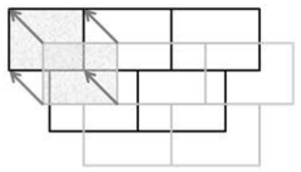
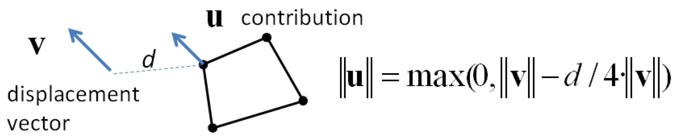
In the first two proposed constraints, only the features close to matched points (i.e., to displacement vectors) are constrained, the other features being conflated only by shape preservation and data consistency constraints. In the first constraint, the influence of displacement vectors is local: only the closest vertex of the close features, to a displacement vector, is constrained by this displacement vector. The search radius is proportional to the vector length (a “5 times length” threshold was used in our implementation). The vertex is constrained with the same direction as the vector but the length is absorbed proportionally to distance, with a factor (4 is proposed) that slows the absorption (Figure 8). This constraint is sufficient when the positional shift between the conflated datasets is low and is effective when the number of previously matched features is low.
Figure 8. Conflation constraint 1: contribution of the displacement vector to the closest vertex of close features.
Ijgi 02 00621 g008
The second constraint is very similar to the first one as the constrained features and vertices are the same. The difference lies in the way the contribution norm is computed (Equation (7)), which absorbs more quickly the displacements. This constraint is preferred to the first one when the positional shift between datasets is large, as it avoids unexpected deformations.
Ijgi 02 00621 i007
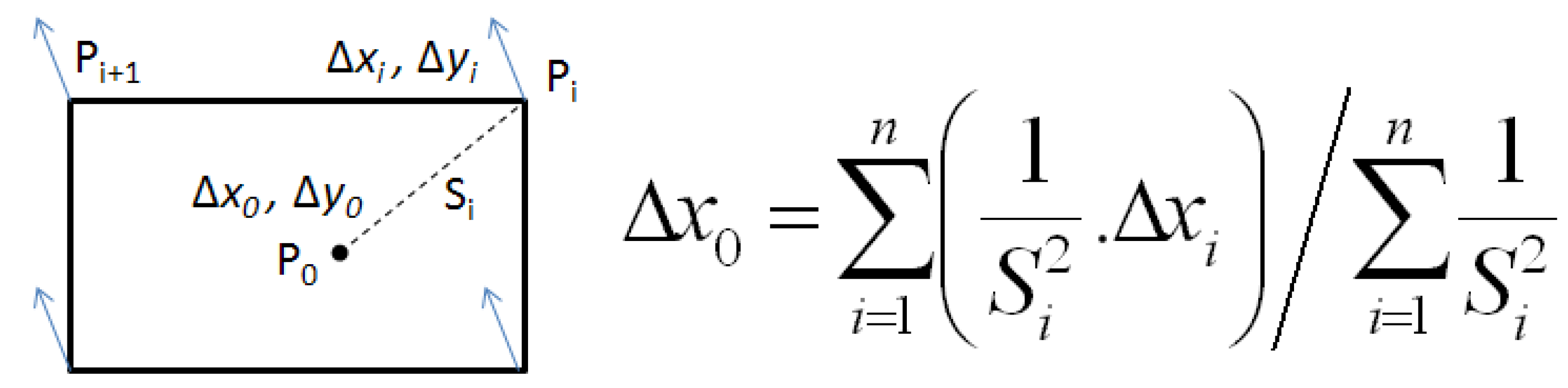
The third constraint is inspired from the rubber sheeting conflation method and is applied on every vertex of every conflated feature. Every vector contributes in an inverse proportional way to the computation of the propagation in a given point (Figure 9). This constraint is particularly effective in datasets where the positional shift between the datasets is large, as the big deformation is propagated and absorbed by a bigger number of features.
Figure 9. Computation of the contribution of displacement vectors in a given point P0.
Ijgi 02 00621 g009
For the three constraints, the linear equations on the constrained points are very simple, for a vector u that aggregates the displacement vectors contributions:
Ijgi 02 00621 i008

3.2.4. Constraints to Maintain Data Consistency

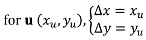
The previous sections propose constraints that allow a conflation that preserve the initial shape of geographic objects. But geographic objects are not isolated in a dataset and share relationship, particularly topological and proximity relations. Our least squares based conflation framework allows preserving these geographic relations thanks to dedicated constraints; three constraints are presented in this section. None is dedicated to topology preservation as topology preservation is inferred in our framework: when features share geometries, their common vertices are only taken into account once in the adjustment and when geometries are transformed by adjustment results, one vertex displacement modifies all features that share the vertex.
The first presented constraint preserves proximity relations between conflated features, i.e., the inter-distance between conflated features does not greatly increase nor decrease. This constraint is inspired from the spatial conflicts constraints from Harrie and Sester [23,24] that ensure a minimal distance between feature symbols. The constraint relies on the computation of neighborhoods for every feature to identify the initial proximity relations. As in [23,24], the neighborhood computation is based on a constrained Delaunay triangulation [27,28] of the features vertices (and constrained by the features segments). The triangulation graph is pruned to identify real proximities (Figure 10): edges inside features are dropped as well as too long edges (if features are too far, it is not a proximity relation!). Like Harrie’s method [23], the remaining edges allow introducing two kinds of constraints: point-to-point constraints and point-to-segment constraints. When edges represent the shortest distance between two features (case 3 in Figure 10), a segment length constraint (Equation (6)) is put on the extreme points of the edge (point-to-point distance). When the distance between two features separated by a triangle is less than the shortest edge between them (case 4 in Figure 10), a point-to-segment constraint is introduced, which deals with the three nodes of the triangle. The distance to preserve is the distance between the single point and the middle of the two other points. This distance expressed with the coordinates of the three points is not linear [23], so the derivative is used like in (Equation (6)) to get the linear equation that preserves this distance.
Figure 10. Constrained Delaunay triangulation used to identify proximities: (1) dashed edges dropped because inside objects, (2) edge dropped as distance > threshold, (3) black edges used for point-to-point proximity, (4) grey edges used for point-to-segment proximity.
Ijgi 02 00621 g010
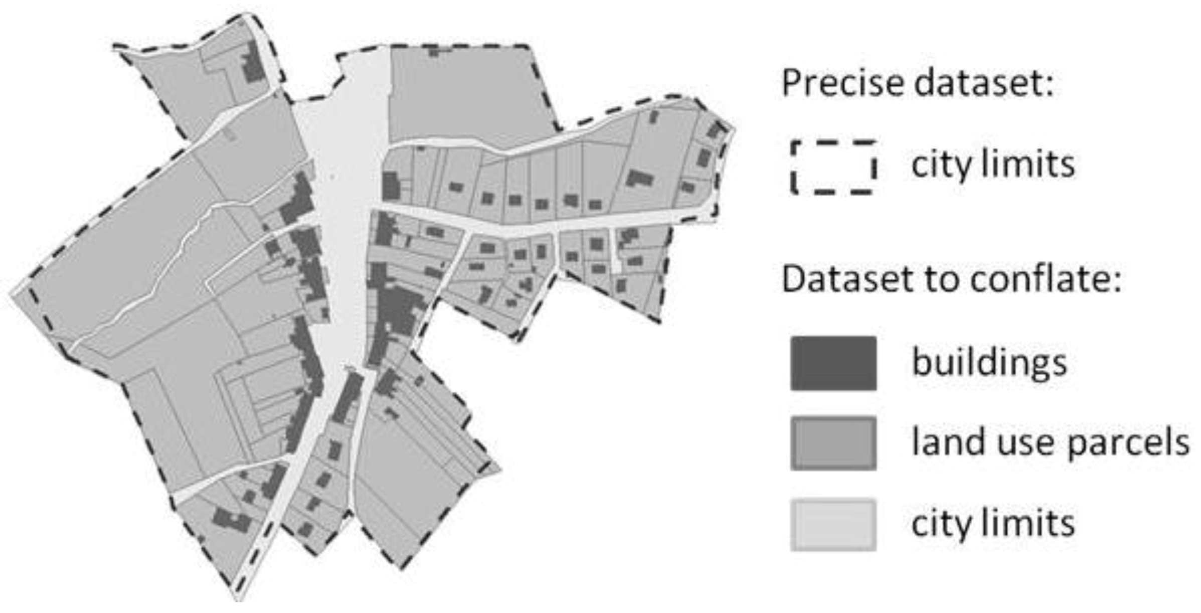
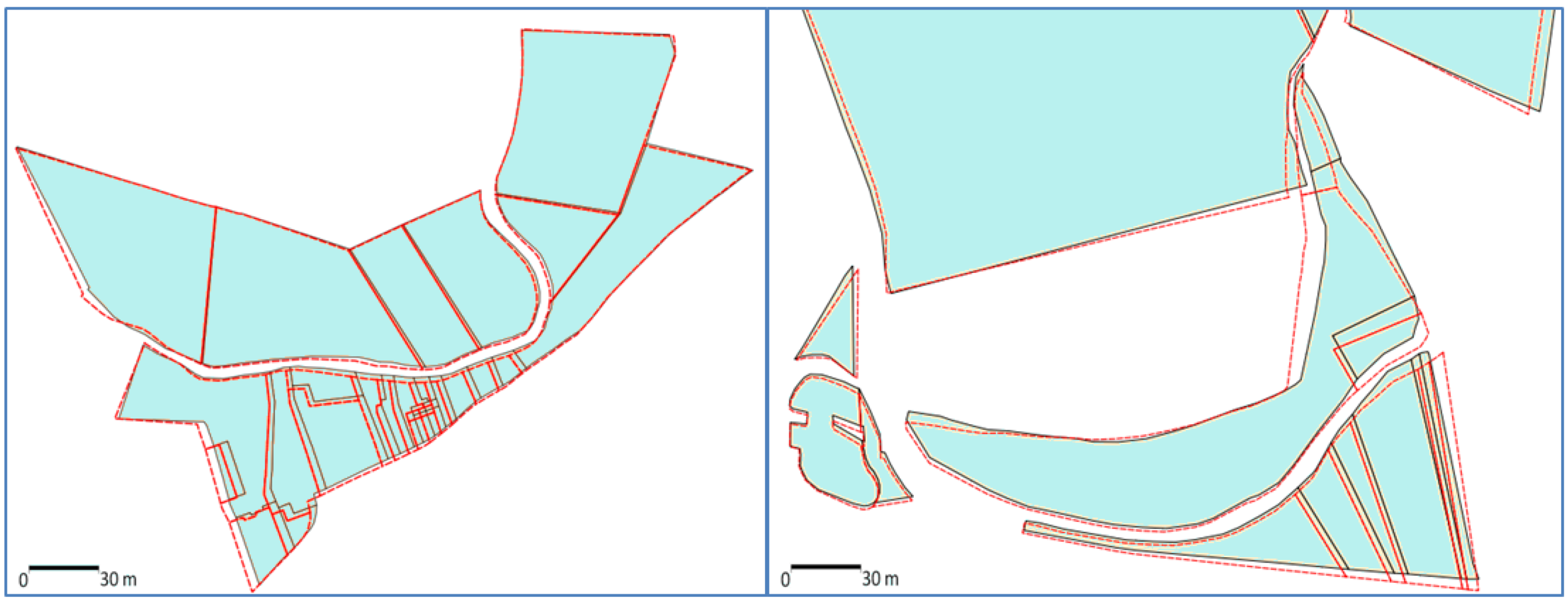
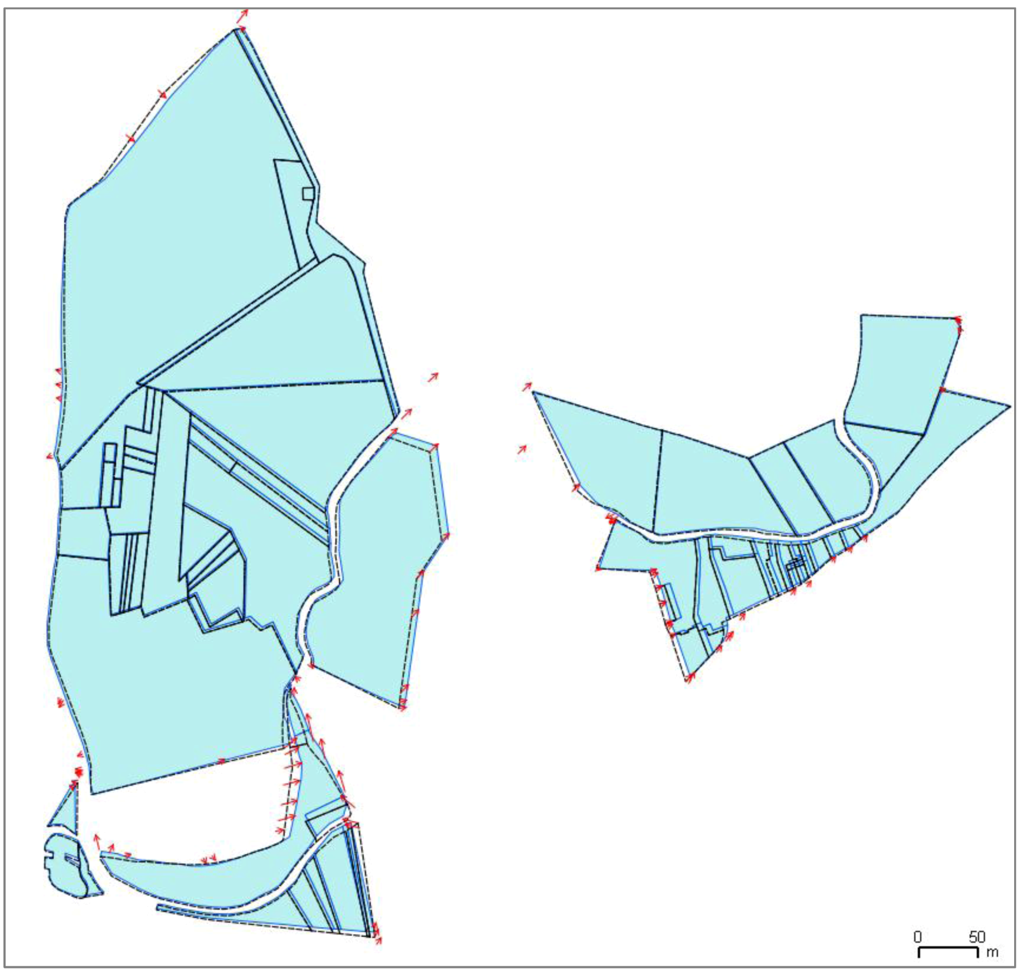
In order to preserve relations with features that are not part of conflation (for instance, additional features in the most detailed dataset), the same type of constraint can be adapted. The same neighborhood computation principle is used but equations are simpler in the derivative computation, as the vertices of the non-conflated features are fixed (the derivative of their coordinates is zero). In the test case presented in the results section, land use parcels are conflated with a more detailed dataset that contains precise city limits, in which the parcels are conflated and a road network with good positional accuracy. The proximity between parcels and roads is preserved so that parcels might not cross roads.
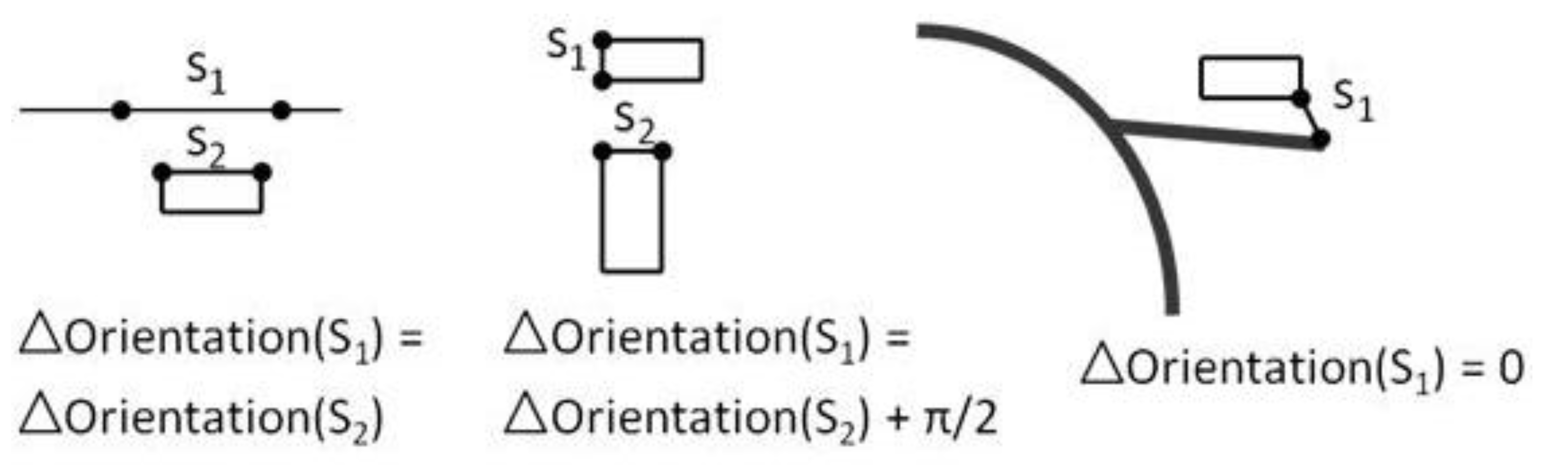
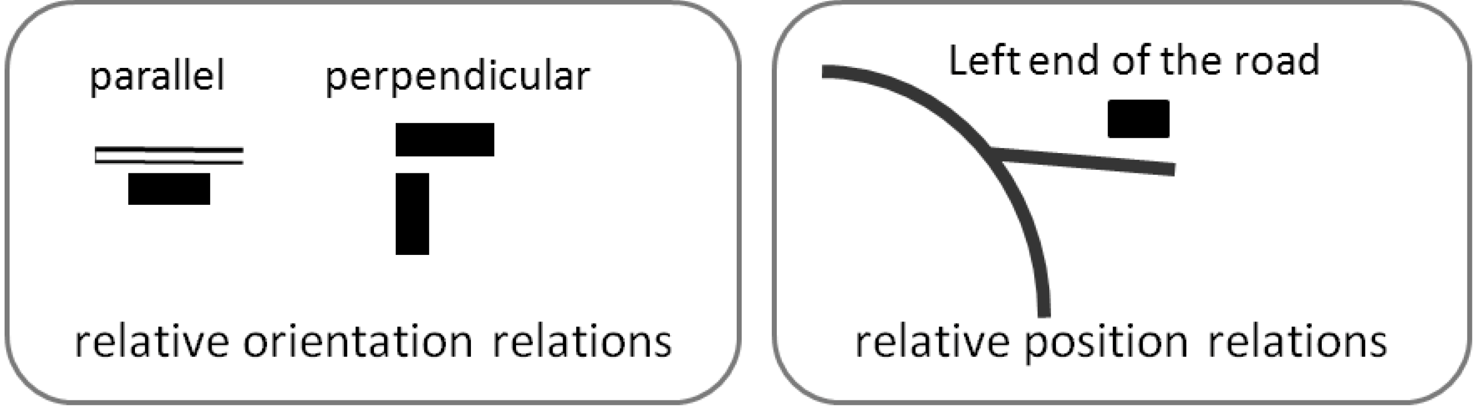
In addition to proximity relations, it may be important to preserve relative orientation relations (e.g., a building parallel to a road, buildings whose main orientation is perpendicular, etc.) and relative position relations (e.g., a building is at the left end of dead end road) (Figure 11). The proposed conflation framework contains constraints to preserve each of the three kinds of relations.
Figure 11. Examples of relative orientation and position relations to preserve during conflation.
Ijgi 02 00621 g011
As with the proximity relations, these relations should first be identified in the initial data, and then the constraints are applied to the related features. The relative position relation is identified each time there is a proximity relation (identified by triangulation) between features that are prone to this kind of constraints (e.g., a dead end and a building). The identification of relative orientation relations is also based on proximities and relies on the measure of the general orientation of polygons [29]: when the general orientations of two close features are either parallel or perpendicular, a constraint is added.
Figure 12 describes how both constraints are transformed into linear equations on feature vertices. The orientation of the chosen segments is computed as in Figure 5 and linearized as in Equation (6).
Figure 12. Constraint expression of the preservation of relative orientation and position relations.
Ijgi 02 00621 g012

3.2.5. Propagation of Additional Data

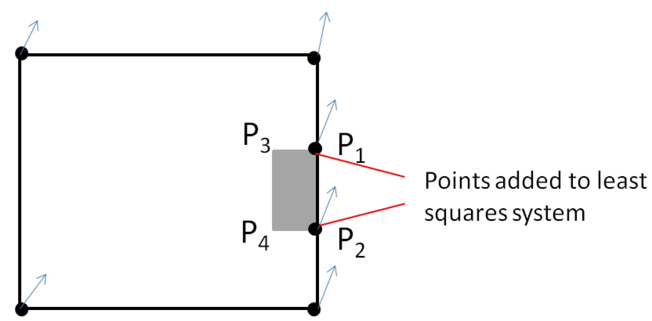
The experiments will show that the least squares conflation framework may generate very large equation systems that could slow computation down or even prevent the solution from being computed. In order to avoid too large systems, the framework allows excluding features from least squares conflation and applying to the excluded features propagation mechanisms from the least squares solution. Two kinds of mechanisms are proposed, one for features topologically connected to conflated features and one for features that are inside or near conflated features.
Both mechanisms rely on the computation of vectors from the least squares displacements. Every vector contributes in an inverse proportional way to the computation of the propagation in a given point (Figure 9), like in the third conflation constraint, or like in the rubber sheeting processes.
In order to allow a propagation on additional features topologically connected to conflated features, which preserves the topological connection, the framework identifies the topological relationships before the conflation. Therefore, topological connection points are added to the geometry points that are constrained. This addition is automatically done in the implemented framework, benefiting from the GIS capabilities of the platform. Then, the least square solution on the connected points is applied to both features. The remaining points of the propagated features are displaced as in Figure 9, considering only the vectors of the connected points (Figure 13). If the connected points have quite different displacement vectors, the propagated feature may be distorted. Nevertheless, it is preferred to preserve topology rather than shape here, as preserving both is not possible. Added to that, if the least squares conflation does preserve shape, the case with quite different vectors on connected points will not occur.
Figure 13. Propagation for topologically connected objects: the connected points are added to the system and a propagated displacement is applied to the remaining points (P3 and P4).
Ijgi 02 00621 g013
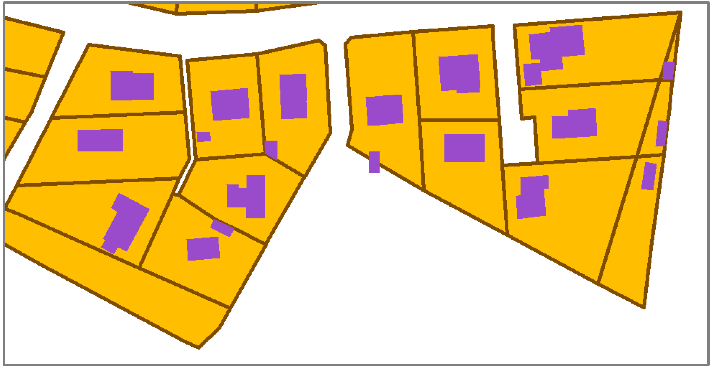
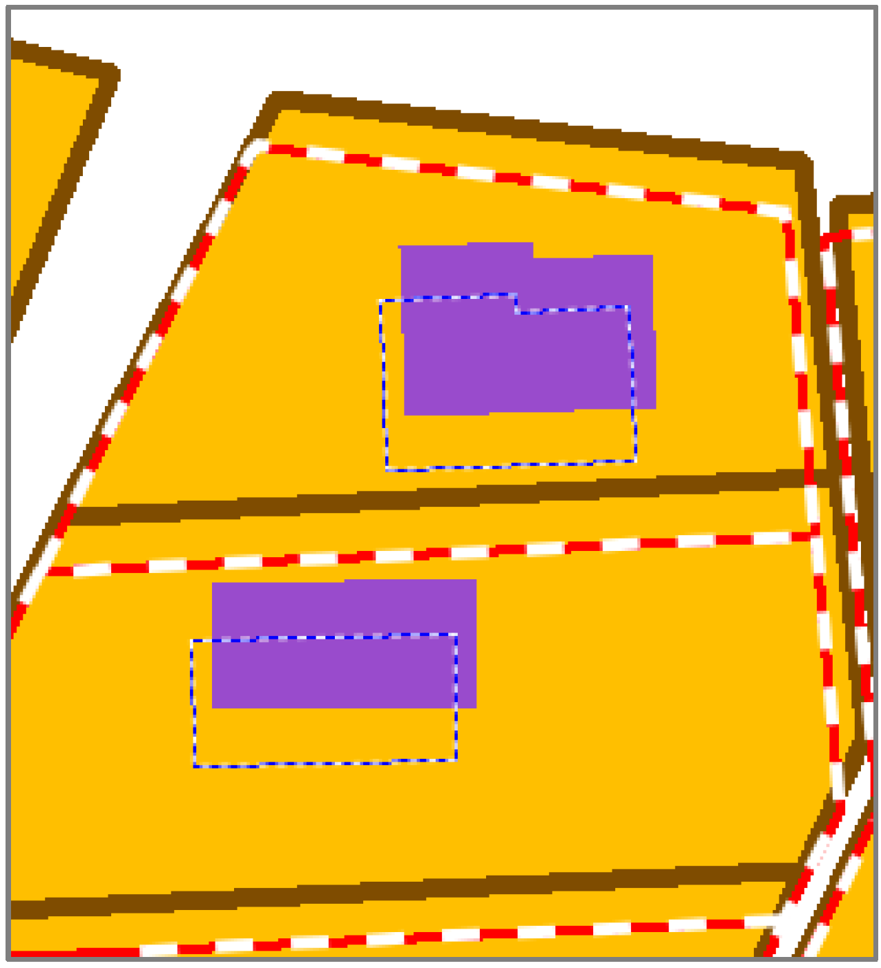
For the additional objects that are not topologically connected to features conflated by least squares (i.e., features inside or near conflated features), a propagation is computed as in Figure 9 on the centroid of the features. Then, the features are simply translated using the centroid propagation, preserving their initial shape.
The decision on which features to propagate and which features to adjust requires knowledge of the use case. Therefore, we leave this decision to the user. However, some general rules to choose can be enunciated:
  • Only unmatched features should be propagated.
  • Small features and rigid features like should be preferred for propagation as such features often need fewer distortions.
  • Features inside conflated features are good candidates for propagation, as it provides accurate propagation vectors.

4. Experiments

The shape preserving conflation framework has been tested thoroughly as experiments have been carried out on a use case with large datasets and real data. The next section describes the use case with land use parcels and buildings. Then, the implementation of the framework is presented and scaling issues are discussed. Finally, some results are presented, evaluated, and discussed.

4.1. Use Case: Land Use Data Conflation

The use case is the conflation of two datasets, a very accurate one containing city limits and network information like roads, paths and rivers; and a less accurate dataset that contains less accurate city limits but also cadastral land use parcels and a building layer, topologically consistent with the parcels. The issue is, thus, to snap the second dataset to the first one’s city limits, preserving consistency with the network elements. Figure 14 shows an extract of the second dataset, containing the parcels and buildings (networks are not displayed for the sake of legibility). This corresponds to a real problem in the French National Mapping Agency that was dealt with our conflation framework.
Figure 14. Extract of the less accurate dataset of the use case, to conflate with accurate city limits.
Ijgi 02 00621 g014
In this use case, the city limits and the parcels are included in the least squares conflation and the buildings are considered as additional propagated features. As this work only focused on geometrical conflation, we did not use one of the matching techniques presented in the related work section. To save time, the data matching is manually carried out between the two layers existing in both datasets, i.e., the city limits. Here, the result of matching is a set vertex pairs, as there is only one city limit feature in each dataset. This matching could be made automatically using the techniques presented in Section 2.
Three areas covering different kind of cities are conflated with both datasets of the use case. One area is quite small with a rural town (Figure 14) that contains some parcels with rectangular shapes and some with smooth shapes (fields delimited by rivers). It contains 100 parcels and 160 buildings. The second dataset is very rural with few buildings but very large parcels with complex shapes (i.e., fields). It contains 70 parcels and 25 buildings. The last area covers a small and dense town with many small and/or thin parcels. It contains 920 parcels and 930 buildings. Moreover, this last area has quite large deformations due to shifts between conflated datasets.

4.2. Implementation

4.2.1. Least Squares Adjustment Model

The conflation framework presented in Section 3 is implemented in Java, in the cartographic generalization platform CartAGen [30], which is Open Source. Thus, it benefits from the large library of geometrical algorithms of CartAGen. The implementation of the framework is as modular as possible. First, matrix computing, necessary for the least squares adjustment, has been interfaced, in order to use any existing matrix API (two APIs are included in the implementation). Then, interfaces have been developed to ease the addition of new internal (i.e., that preserve shape) and external (i.e., that conflate or preserve relations) constraints.
The implementation provides a GUI to define the parameters (e.g., the constraints used, the weights, the input data,...) and trigger the conflation. A scheduler was developed and it sequences the steps of the conflation: build the points (i.e., the unknown) that will be conflated, compute the constraints on each point, transform the constraints into the linear equation system, solve the system by adjustment and finally apply the deformations to features.
To control a conflation with the GUI, the user simply defines the internal constraints for each feature type, the external constraints, constraints weights, and finally the features that are propagated rather than adjusted. As many constraints are available, a user has to tune the framework to determine the correct parameterization for a use case. For our use case, experiments showed that propagating buildings was successful, so it was decided that including them in the adjustment was not necessary. The experiments allow the inference of some criteria to define constraints weight:
  • the chosen conflation constraint should have very high weights (20 in the experiment),
  • key shape constraints like stiffness for parcels should have high weights (16 in the experiment),
  • the movement constraint should have a minimal weight (1 in the experiment).

4.2.2. Scalability Issues

With such a use case that contains many land use parcels, the number of equations in the least squares system may quickly become very large. For instance, the conflation of a dataset with 110 land use parcels, which corresponds to 1,400 unknowns (i.e., 700 vertices) in the framework, uses a 1,400 × 1,400 matrix to inverse. It involves the handling of very large matrices that overloaded the implemented Java APIs. Two complementary solutions were developed to overcome this difficulty to handle large datasets: partition data and use sparse matrices.
The first solution to compute large datasets is to partition data into smaller parts that are computed separately. In order to avoid topology disconnections, partitioning has to take topology into account: land use parcels are grouped when they are topologically connected (Figure 15), and each group is conflated separately with its own equation system. Nevertheless, the proximity constraints between disconnected parcels are computed at the beginning of the process, in order to really preserve the initial inter-distance. When such separations of features do not exist in a conflated dataset, two general rules should be followed:
  • Features that share topology and spatial relations should be grouped in a partition.
  • Constraints between features at the edge and features outside the partition should be included in the adjustment.
Figure 15. Disconnected sets of land use parcels that can be partitioned and treated separately.
Ijgi 02 00621 g015
Added to the partitioning, the implementation was changed to introduce sparse matrices in the least squares adjustment. Sparse matrices are matrices with a lot of zero values. The storage of such matrices is much lighter than standard matrices [31] and the Jacobean matrix in the least squares framework contains many zeros so can be stored as sparse matrix. The experiments show that combining partitioning and sparse matrices allows the efficient computation of very large datasets, as sparse matrices also quicken resolution.

4.3. Results

Conflation results are presented for the use case with two different cities that present variations in size, shapes, and deformations required. Only results on small cities are presented to keep the figures readable because most distortions are negligible compared to city size for large cities, and would not be readable at the city scale. The first result is presented in Figure 16 for a small town (110 features, 700 points) with minor deformations (small conflation vectors), as the datasets are very close to each other. In Figure 16, some vectors may not be connected to a parcel node because they are computed on city limits, which are not always connected to a parcel (parcels only are conflated). The land use parcels are mainly big and straight (cultivated fields). Figure 16 shows that both man-made and natural shapes are well preserved, as well as parcels proximity. There is no parcel layer in the reference dataset to compare to, so the quality of conflation should be assessed according to the shape preservation despite the needed distortions.
The second city is characterized by large distortions (10 to 15 m), and quite complex shapes, and the conflation results remain excellent (Figure 17). Figure 17 shows zoomed extracts of Figure 18 that confirm that complex shapes (e.g., curved shapes, or very thin shapes) and proximity relations are well preserved by the least squares conflation framework, despite large distortions.
Figure 16. Conflated parcels (dashed lines for initial data) extracted from the Figure 14 (area with small distortion, the arrows show some matching vectors) (1) polygon shapes are well preserved, (2) small spaces between parcels are preserved, (3) even curve spaces due to rivers are preserved.
Ijgi 02 00621 g016
Figure 17. Zoomed extracts of the second conflated city: despite large distortions, complex shapes are well preserved.
Ijgi 02 00621 g017
In order to improve the legibility of the presented results, the buildings propagation was excluded from the previous result pictures. Figure 19, Figure 20 show some results for the propagation of either topologically connected buildings or simple buildings inside parcels. The results show that the local propagation of additional data is quite effective because topology is preserved without shape distortion (Figure 20) and the relative position of the buildings in the parcel is preserved (Figure 19).

4.4. Evaluation

In order to evaluate the results obtained with the least squares conflation framework on the test cases, they are compared to the results of the rubber sheeting method on the same test case. The rubber sheeting interpolation is a simple inverse distance weighting, as proposed by Haunert [16], which computes a displacement field (no triangulation involved). Figure 21 shows the conflation of features close to the displacement vectors inferred by matching. There, the rubber sheeting conflation deforms features without shape preservation, contrary to least squares conflation, because the vectors are quite large.
Figure 18. Conflation results with data that require large distortions (conflated parcels are in plain blue, initial outlines are dashed and arrows show matching vectors).
Ijgi 02 00621 g018
Figure 19. Propagation of the least squares conflation to buildings inside parcels: Initial geometries drawn with dashed lines.
Ijgi 02 00621 g019
Figure 20. Other examples of propagated buildings, including buildings topologically connected to conflated parcels.
Ijgi 02 00621 g020
Figure 21. (1) Comparison of the least squares based conflation (in plain colors), the rubber sheeting conflation (with dots) and the initial data (with dashes); (2) a broader view of the initial data with deformation vectors.
Ijgi 02 00621 g021
Conflation methods were also compared by automatic measuring of shape preservation: the shape of the conflated features was compared to the shape of the corresponding initial features (the framework maintains links between features). Five measures are used: area increase ratio that measures if the conflation increased or decreased the feature area, the surface distance (Figure 1) that measures the similarity of shapes, the turning function [7] that measures the preservation of angles independently to translations, the polygon signature [8] that measures the similarity of shapes independently to translations, and the Hausdorff distance [6] that measures the similarity of contour (Table 1). The table shows how least squares conflation better preserves shape: the surface distance is bigger because of the translation implied by the shape preservation constraints, but the turning function distance is twice smaller in RMS error, which means that angles are better preserved. Polygon signature and Hausdorff distance RMS errors are also much better with the least squares conflation that increases less the area of the features. So, the visual evaluation is confirmed and the least squares conflation better preserves shape than rubber sheeting.
Nevertheless, some defects have been noticed in one of the conflated areas, around large displacement vectors: when the segments of the conflated polygons are very large (Figure 22, case 1), the stiffness constraint does not work very well, as the enlargement of the segment implies too big residual vectors. The solution to fix the defect is to add vertices in segments that are too long (i.e., Steiner points), to avoid such a situation. The stiffness constraint has another defect with very small segments (Figure 22, case 2): as the segments length is very small, big deformations considered to its size, e.g., with big angle variation, lead to small residual vectors judged as acceptable by the least squares adjustment. A solution to fix the defect is to add an orientation preservation constraint with a huge weight on the very small segments, to ensure the preservation of the angles with the connected segments.
Table 1. Root Mean Square errors (RMS) for Least Squares conflation (LS) and Rubber Sheeting conflation (RS) compared to initial data, for five shape comparing measures and 200 features.
RMS Error LSRMS Error RS
Area increase ratio3.39%5.48%
Surface distance0.1520.102
Turning function0.0930.184
Polygon signature0.5360.932
Hausdorff distance3.0873.736
Figure 22. Initial data to conflate where the identified two defects (very long (1) and very short (2) segments with large distortions) may occur.
Ijgi 02 00621 g022
As mentioned earlier, the use case does not contain any ideal final data to compare with the conflated result as the land use parcels are not in the precise dataset. In order to cope with this situation in the framework evaluation, benchmark data were created in a GIS with initial and final parcels and the vectors of the transformation (Figure 23). The least squares conflation framework was compared to the rubber sheeting method to conflate such data. Results show that the least squares framework performs a little better than rubber sheeting for positioning and area preservation and much better for shape preservation. It is attested to by the turning function and polygon signature measures in comparison to the benchmark final data.
Figure 23. (1) Conflation benchmark data (2) least squares and rubber sheeting results compared to benchmark final data.
Ijgi 02 00621 g023
A final way to evaluate the framework is to analyse its sensitivity to its parameters: the choice of the constraints and the weights assigned to each constraint. Different test conflations were carried out with varying constraints and weight-settings. Weight-setting in the framework is a challenging task as it is in the least squares based generalization [25]. Figure 24 shows the comparison of several conflations with varying parameters: the standard parameters, a conflation with weights randomly slightly different from the standard ones, a conflation with very different weights, and a conflation using the conflation constraint number 2 instead of number 1. The variations are visually significant when the conflation constraint is changed or when the weights are drastically changed. However, the shape variations mainly appear near the displacement vectors due to matching and most of features are conflated similarly which is confirmed by the surface distance between the standard conflation and the alternative ones. The root mean square distances is low for both weight variations (0.06 and 0.08 while it is 0.15 with the initial features) but is quite significant for the conflation constraint alternative (0.15) which confirms that the choice of the conflation constraint really impacts conflation results. Thus, this choice should be made carefully, using experimentations.
Figure 24. Conflation variations with varying parameters.
Ijgi 02 00621 g024

4.5. Discussion

The presented shape preserving conflation framework is computationally intense, so computation time needs to be discussed. As mentioned earlier, the first dataset (Figure 14) has 110 land use parcels, which corresponds to 1,400 unknowns (i.e., 700 vertices) in the framework, and the constraints used lead to a 13,000 × 1,400 Jacobean matrix (i.e., matrix A) to process. The matrix to inverse, ATPA is 1,400 × 1,400. On a very standard desktop computer, the conflation takes approximately two minutes with the standard Java matrix API, but less than five seconds when using the C sparse matrix API. The second dataset presented in the results contains less features (70) but larger parcels, with more vertices (Figure 18). The computation time, there, is a bit faster so large and complex features do not slow conflation computation. The framework was also tested on a much larger dataset, with 930 features including very large parcels. Computation takes less than one minute with the sparse matrix API, but the increase of computation time is not due to the adjustment but to the proximities computation. Indeed, filtering the triangulation edges to define proximities has Ο(n2) complexity due to implementation issues. If we include the required matching process in the computation time, there is no drastic change: an automatic matching technique was tested between initial parcels and conflated parcels of the test datasets, and the processing time is negligible compared to conflation computation time. More complex matching processes may take more time but should not drastically increase the total computation time.
The requirement for matching should also be discussed. Only one matched feature is necessary to conflate a dataset but such minimal matching does not allow a conflation as accurate as a more complete vertex to vertex matching. Indeed, the more vertices are matched, the more precise the conflation constraints are. However, this can be counterbalanced by the use of an appropriate conflation constraint: if there are few displacement vectors, the conflation constraint to choose has to have a large impact radius for each vector.
Furthermore, one of the hypotheses of the conflation framework is that a less precise dataset is conflated on a reference dataset, whose positional accuracy is better. But it is not always possible to determine a reference dataset. As it is modeled and implemented, the framework only allows choosing one of the datasets as the reference and conflating the other on it. However, it seems feasible to define constraints to conflate both datasets to a medium geometry, replacing the conflation constraints based on displacement vectors.
The proposed least squares based conflation framework is a contribution to geometrical conflation methods as it allows to preserve geographic shapes during conflation, which was not possible before. There are also slighter contributions to the least square based methods that are used in generalization for instance: some new constraints to preserve spatial relations have been introduced, techniques like partitioning or sparse matrices used to reduce matrices complexity could be used to apply least squares based generalization methods to larger zones. The way it integrates rubber-sheeting propagation could be useful in generalization too. In addition to the defects identified in the evaluation section, the framework has some drawbacks, the major one being the complexity of the parameterization, i.e., choosing and weighting the constraints in a specific use case. Weight setting is clearly not intuitive and extensive testing is required to identify the good weights for a test case. For instance, the case study presented in this paper required ten or so tries to find the best weights. Fortunately, if computing time is low, the cost of weight setting is not so high. The other drawback lays in the least squares principles: errors are, in a way, averaged on all equations (i.e., constraints), weighting being the only way to make some important constraints mostly satisfied and less important constraints less satisfied.

5. Conclusions

To conclude, this paper dealt with the proposition of a new framework to geometrical conflation that preserves geographic shapes while deforming conflated features. The framework is based on the least squares principles that were successfully used in map generalization, by Harrie [23] and Sester [24]. The framework allows to preserve different kinds of shapes (i.e., man-made or natural) and different kind of relations between features (proximity, relative orientation), in an optimized solution. The framework has been implemented in Java and tested for the conflation of land use data, with quite large datasets. The evaluation of the results, compared to the rubber sheeting technique, prove the efficiency of such a method.
To go further, the least square based conflation framework should be tested on the conflation of use cases with quite different data to verify its genericity in the preservation of geographic shapes. Then, it could be extended by new constraints to preserve additional kinds of shape or geographic relations. Moreover, the framework is only dedicated to conflation cases with a dataset used as the geometrical reference. As a consequence, it is not directly usable in cases where the datasets have similar accuracies. An extension of the framework should be developed to allow shape preserving conflations in such cases. Finally, it could be interesting to investigate the use of hard constraints in a least squares adjustment, shifting from Gauss-Markov least squares model to Gauss-Helmert model.

Conflict of Interest

The authors declare no conflict of interest.

References

  1. Kilpeläinen, T. Maintenance of multiple representation databases for topographic data. Cartogr. J. 2001, 37, 101–107. [Google Scholar] [CrossRef]
  2. Adams, B.; Li, L.; Raubal, M.; Goodchild, M.F. A General Framework for Conflation. In Proceedings of Sixth International Conference on Geographic Information Science, Zurich, Switzerland, 14–17 September 2010.
  3. Goodchild, M.F. Citizens as voluntary sensors: Spatial data infrastructure in the world of web 2.0. Int. J. Spatial Data Infrastruct. Res. 2007, 2, 24–32. [Google Scholar]
  4. Saalfeld, A. Conflation: Automated map compilation. Int. J. Geogr. Inf. Syst. 1988, 2, 217–228. [Google Scholar] [CrossRef]
  5. Walter, V.; Fritsch, D. Matching spatial data sets: A statistical approach. Int. J. Geogr. Inf. Sci. 1999, 13, 445–473. [Google Scholar]
  6. Abbas, I. Base de Données Vectorielles et Erreur Cartographique: Problèmes Posés par le Contrôle Ponctuel; une mÉthode Alternative Fondée sur la Distance de Hausdorff. Ph.D. Thesis, Université de Paris, Paris, France, 1994. [Google Scholar]
  7. Arkin, E.M.; Chew, L.P.; Huttenlocher, D.P.; Kedem, K.; Mitchell, J.S.B. An efficiently computable metric for comparing polygonal shapes. IEEE Trans. Patt. Anal. Mach. Int. 1991, 13, 209–216. [Google Scholar] [CrossRef]
  8. Vauglin, F.; Bel Hadj Ali, A. Geometric Matching of Polygonal Surfaces in GISs. In Proceedings of ASPRS Annual Meeting, Tampa, FL, USA, 30 March–3 April 1998.
  9. Mascret, A.; Devogele, T.; Berre, I.; Henaff, A. Coastline Matching Process Based on the Discrete Fréchet Distance. In Progress in Spatial Data Handling; Riedl, A., Kainz, W., Elmes, G.A., Eds.; Springer: Berlin/Heidelberg, Germany, 2006; pp. 383–400. [Google Scholar]
  10. Mustière, S.; Devogele, T. Matching networks with different levels of detail. GeoInformatica 2008, 12, 435–453. [Google Scholar]
  11. Samal, A.; Seth, S.; Cueto, K. A feature-based approach to conflation of geospatial sources. Int. J. Geogr. Inf. Sci. 2004, 18, 459–489. [Google Scholar] [CrossRef]
  12. Olteanu Raimond, A.M.; Mustière, S. Data Matching—A Matter of Belief. In Headway in Spatial Data Handling; Ruas, A., Gold, C., Eds.; Springer: Berlin/Heidelberg, Germany, 2008; pp. 501–519. [Google Scholar]
  13. Li, L.; Goodchild, M.F. Optimized Feature Matching in Conflation. In Proceedings of Sixth International Conference on Geographic Information Science, Zurich, Switzerland, 14–17 September 2010.
  14. Ware, J.M.; Jones, C.B. Matching and Aligning Features in Overlayed Coverages. In Proceedings of the 6th ACM International Symposium on Advances in Geographic Information Systems, New York, NY, USA, 6–7 November 1998; ACM Press: New York, NY, USA; pp. 28–33.
  15. Laurini, R. Spatial multi-database topological continuity and indexing: A step towards seamless GIS data interoperability. Int. J. Geogr. Inf. Sci. 1998, 12, 373–402. [Google Scholar] [CrossRef]
  16. Haunert, J.H. Link Based Conflation of Geographic Datasets. In Proceedings of 8th ICA Workshop on Generalisation and Multiple Representation, La Coruña, Spain, 7–8 July 2005.
  17. Haunert, J.H.; Anders, K.H.; Sester, M. Hierarchical Structures for Rule-Based Incremental Generalisation. In Proceedings of the ISPRS Archives XXXVI Working Group II/2, Beijing, China, 3–11 July 2008.
  18. Kampshoff, S. Mathematical Models for Geometrical Integration. In Proceedings of the First International Workshop on Next Generation 3D City Models, Bonn, Germany, 21–22 June 2005.
  19. Gruendig, L.; Gielsdorf, F.; Aschoff, B. Merging Different Data Sets Based on Matching and Adjustment Techniques. In Proceedings of Strategic Integration of Surveying Services-FIG Working Week, Hong Kong, China, 13–17 May 2007.
  20. Cobb, M.A.; Chung, M.J.; Foley, H.; Petry, F.E.; Shaw, K.B.; Miller, H.V. A rule-based approach for the conflation of attributed vector data. GeoInformatica 1998, 2, 7–35. [Google Scholar]
  21. Bjerhammar, A. Theory of Errors and Generalized Matrix Inverses; Elsevier: Amsterdam, The Netherlands, 1973. [Google Scholar]
  22. Beard, K.M. Constraints on Rule Formation. In Map Generalization; Buttenfield, B., McMaster, R., Eds.; Longman Pages: London, UK, 1991; pp. 121–135. [Google Scholar]
  23. Harrie, L.E. The constraint method for solving spatial conflicts in cartographic generalization. Cartogr. Geogr. Inf. Sci. 1999, 26, 55–69. [Google Scholar] [CrossRef]
  24. Sester, M. Optimization approaches for generalization and data abstraction. Int. J. Geogr. Inf. Sci. 2005, 19, 871–897. [Google Scholar] [CrossRef]
  25. Harrie, L.E. Weight-Setting and quality assessment in simultaneous graphic generalization. Cartogr. J. 2003, 40, 221–233. [Google Scholar] [CrossRef]
  26. Legrand, C.; Duchêne, C.; Lecordix, F. Propagation of the Displacements and Deformations during a Generalisation Process. In Proceedings of International Cartographic Conference, ICA, La Coruña, Spain, 9–16 July 2005.
  27. De Berg, M.; van Kreveld, M.; Overmars, M.; Schwarzkopf, O. Computational Geometry: Algorithms and Applications, 2nd ed; Springer: Berlin/Heidelberg, Germany, 2000. [Google Scholar]
  28. Shewchuk, J.R. Triangle: Engineering a 2D Quality Mesh Generator and Delaunay Triangulator. In Applied Computational Geometry: Towards Geometric Engineering; Lin, M.C., Manocha, D., Eds.; Springer-Verlag: Berlin, Germany, 1996; pp. 203–222. [Google Scholar]
  29. Duchêne, C.; Bard, S.; Barillot, X.; Ruas, A.; Trevisan, J.; Holzapfel, F. Quantitative and Qualitative Description of Building Orientation. Proceedings of 5th Workshop on Progress in Automated Map Generalization, Paris, France, 28–30 April 2003; 2003. Available online: http://aci.ign.fr/BDpubli/paris2003/papers/duchene_et_al_v1.pdf (accessed on 3 April 2013).
  30. Renard, J.; Gaffuri, J.; Duchêne, C.; Touya, G. Automated Generalisation Results Using the Agent-Based Platform CartAGen. In Proceedings of 25th International Cartographic Conference (ICC’11), Paris, France, 30 June–1 July 2011.
  31. Pissanetzky, S. Sparse Matrix Technology; Academic Press: Waltham, MA, USA, 1984. [Google Scholar]

