Article

FumeBot: A Deep Convolutional Neural Network Controlled Robot

School of Engineering, Newcastle University, Newcastle upon Tyne NE1 7RU, UK
*
Author to whom correspondence should be addressed.
Robotics 2019, 8(3), 62; https://doi.org/10.3390/robotics8030062
Submission received: 19 June 2019 / Revised: 19 July 2019 / Accepted: 25 July 2019 / Published: 29 July 2019
(This article belongs to the Section Industrial Robots and Automation)

Abstract

:
This paper describes the development of a convolutional neural network for the control of a home monitoring robot (FumeBot). The robot is fitted with a Raspberry Pi for on board control and a Raspberry Pi camera is used as the data feed for the neural network. A wireless connection between the robot and a graphical user interface running on a laptop allows for the diagnostics and development of the neural network. The neural network, running on the laptop, was trained using a supervised training method. The robot was put through a series of obstacle courses to test its robustness, with the tests demonstrating that the controller has learned to navigate the obstacles to a reasonable level. The main problem identified in this work was that the neural controller did not have memory of past actions it took and a past state of the world resulting in obstacle collisions. Options to rectify this issue are suggested.

1. Introduction

A range of home use robots are currently commercially available including robotic vacuum cleaners [1,2] and lawn mowers [3,4]. Development of autonomous surveillance or home monitoring robots is of great importance, not only for security, but for assisting the elderly [5]. For home surveillance, the additional needs of effective monitoring and remote communication with the user are required [6]. To develop monitoring and surveillance robots for practical implementation in a home environment, a range of issues must be resolved. These include working in cluttered environments [7], the need to perform surveillance in conjunction with simultaneous localization and mapping [8], object recognition and tracking [9], integration of static and mobile surveillance systems [10], and simplifying the computing requirements whilst maintaining fully autonomous monitoring capabilities [11]. In addition, making them truly autonomous in a way that they can act in different scenarios and environments without any human intervention is a challenging task. Deep learning using deep neural networks (DNN) are being applied to solve many complicated tasks where the machine itself will try to learn the task, provided that it has enough data. This approach has achieved amazing results in all sorts of applications from image processing tasks such as object detection [12] and segmentation of images [13], speech recognition [14] and generation [15], and the development of self-driving cars [16]. The possibilities are endless with deep learning in applications from a wide variety of fields including robotics.
A variety of approaches are utilized in applying neural networks to mobile robotic applications, in particular to obstacle avoidance and path planning with most using distance measuring approaches to determine obstacle location. Cost effective approaches utilize sensors such as infrared and ultrasonics. Janglová [17] demonstrated neural network approaches to mapping and path planning by successfully implementing two neural networks on a differential drive robot named Auro containing ultrasound range finders. Similarly, Parhi et al. [18], using a Khepra-III mobile robot equipped with infrared and ultrasonic sensors, demonstrated collision free motion and target seeking in real time in an unknown environment. Higher resolution ranging data may be obtained from laser range finders at the expense of the higher costs involved. Simulation work by Shamsfakhr et al. [19] showed how a SICK laser scanner, used as an input to a neural network, could be used for navigation and obstacle avoidance. Chi et al. [20] implemented a neural network on a Pioneer P3DX robot that required a Hokuyo URG-04LX laser range finder due to the limited reliability of the sonar data. Their work highlights the advantage of using the neural network in real time navigation as computation time is reduced since models of the robot and environment are not implicitly required. Takiguchi et al. [21], using a Hokoyu UTM-X001s laser range finder and a deep learning network, successfully demonstrated object detection and obstacle avoidance on both static and dynamic objects. Another option for obtaining depth measurements is by utilizing a Kinect, as reported by Wu et al. [22] on a Pioneer 3-AT mobile robot. After simulation in Gazebo, the neural network demonstrated autonomous steering in complex real environments. In all these methods, the data input to the neural network is from an active ranging device giving a definitive measurement on the distance to the obstacles. In contrast to this, a novel approach was attempted by Xie et al. [23] utilizing monocular vision only. A Turtlebot was implemented with a camera and simulations built in Gazebo, which were used to train the network. Practical implementation demonstrated successful avoidance of both static and dynamic objects. Similar work utilizing monocular vision but being applied to unmanned aerial vehicles (UAVs) is demonstrated by Yang et al. [24] and Singla et al. [25]. These approaches utilize red-green-blue (RGB) image data to predict depth maps of the environment and then plan trajectories accordingly. Results look promising.
For complex tasks, such as home surveillance, several neural networks may be required. For example, one neural network is used for obstacle avoidance and steering, another neural network is used for localization, whilst a third uses data scans of the environment to highlight any dangerous situations. In this scenario, it can be seen that a single neural network cannot be used to do all the required tasks, and instead, multiple neural networks are used. A fixed algorithm is often needed at the end of the neural network that executes certain actions based on the output of it.
For this project, a robot called FumeBot, which can serve as a prototype home monitoring or surveillance robot, was developed. The main idea behind such a robot would be to set it at home and connect it to a wireless network. It would then perform relevant actions, either autonomously or on receiving a command, possibly via a short message service (SMS). Examples include using simple algorithms to process data from environmental sensors to check for noxious gases to image recognition of thermal images to check whether an elderly person has fallen. Notification of the results are then communicated back. These example scenarios are simple applications but can be expanded to tackle other complex tasks. However, the learning methods that can be used to train neural networks are quite challenging in terms of computation and also implementation. There are a variety of different types of neural network architecture and there are also the different methods of training the neural network.
This report looks into exploring how a relatively simple home surveillance robot could be built and deployed using deep learning approaches to control the actions of the robot for the specific task of navigation and explores the issues that arise when such methods are used.

2. Neural Network Considerations

2.1. Finding a Deep Neural Network for the Application

The type of neural network that is required is one that can work with images, such as a convolutional neural network (CNN), which is used for image recognition and segmentation tasks. The structure of the convolutional net enables it to compensate for shifts and orientation of the image. If a CNN is trained with a set of images as inputs and corresponding controls as labels, the neural network output can then be used to control the motion of a robot. This was demonstrated by Hwu et al. [26] by navigating a mountain trail in which the CNN learned to move away from the green bushes on either side of the path, keeping it in the middle of the trail. Although this method is interesting, the approach cannot be used in an indoor environment where there is no clear trail or lane-type markings that the convolutional net can learn and use to classify the input image to make an appropriate control decision.
Convolutional neural networks have a problem in that they have a high tendency to overfit for the input data in the fully connected layer of the CNN. Dropout is a new concept that was introduced by Hinton et al. [27]. In dropout, neurons are randomly selected, determined by a predefined probability. This can be applied to both hidden layers and the input layer. The selected neurons are removed from the network, together with any corresponding connections to other neurons, for a training iteration. When the neuron is dropped out, they essentially do not take part in the forward and backward propagation. As a result, the neural network is forced to adapt to situations where it cannot depend on neurons in the previous layer. Over the complete training set of data, this has the effect of training different types of neural network architectures at once. Although a larger initial network with a greater number of layers and neurons is required to keep the network from excessively thinning out because of the random dropout, the overall result is essentially an averaging of multiple neural networks, thereby giving good generalization of the data. Regularization [28] is another option and is used to enable the neural network to learn simpler models rather than complex ones. During training, the cost function incorporates a sum of all the weights used in the network. Thus, during training, the neural network is forced to reduce the weights to drive down the cost. In L1 regularization, weights are reduced to potentially a zero value, thus reducing the size of the network. In L2 regularization, weights are reduced to their minimum non-zero value. In both cases, it reduces the complexity of the model and provides better generalization of the data. Krizhevsky et al. [29] utilized these approaches to develop a modified convolutional neural network for successfully classifying a data set consisting of a thousand different categories of images. Another improvement to the standard convolutional net was the use of rectified linear units (ReLU) [30] activation instead of the commonly used sigmoidal function. The use of the ReLU activation function helps with the speed of convergence.

2.2. Neural Network Application Solution

The modified convolutional neural network by Krizhevsky et al. [29] is a good starting point for this project. During the learning phase, the robot will be driven by the user, so additional modifications are required to allow the CNN to relate image data to the corresponding directional movements required by the robot. The image frames are given as input to the CNN and the user’s directional controls are the labels or the ground truth that the network must learn to output.
Data collected for neural network training is typically split into training, validation, and test sets. For this project, the training set needed balancing of the data due to how the robot is driven; for example, if the robot is driven straight forward for an extended period of time with only periodic left and right corrections, then the majority of the data set will be of images that will have the label for the direction control as straight forward when compared to other direction control commands such as left and right. If this dataset is fed to the neural network, the network would quickly learn that the majority of the time it should move forward and occasionally left and right. This might be a desired response from the network if that is what is required for the application but not if the robot is introduced to an obstacle course where it has to make sharp left and right turns; the robot would have a hard time navigating through the obstacle course. In order to prevent the above-mentioned problem, balancing of the dataset is necessary. Another point to note is whether to shuffle the data when training the network instead of just feeding the network input data in the order they were collected. For the convolutional net that is going to be used, the sequence of the data really does not matter and therefore shuffling of the data is an optional choice.
The hyperparameters like the number of layers, number of units or neurons per layer, learning rate, regularization, and many other parameters have to be chosen, but a good starting point would be to use the convolutional net described above. Throughout the process of developing the above convolutional neural network, a stochastic gradient decent is used instead of batch training. In batch training, the entire training examples are used to find the gradient and then update the weight and biases. This method takes a significant amount of time to train the neural network. On the other hand, when using a stochastic gradient descent, mini-batches are used in which random data from the training dataset is collected and then made into a mini-batch of training data. This mini-batch is then fed forward through the network, and then the gradient for this mini-batch is found and the weights and biases in the network are updated. This is a noisier method compared to the batch training but produces much better results and is also faster at finding a convergence [31].

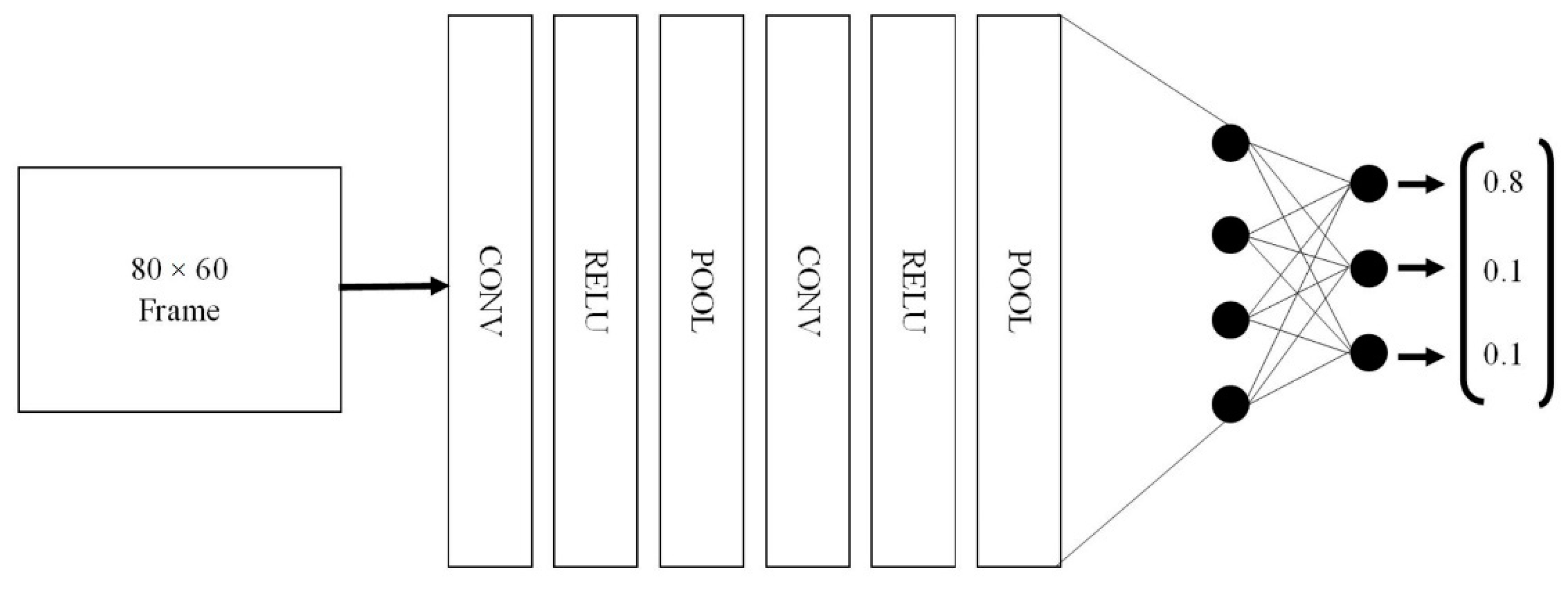
2.3. Setting up the Convolutional Neural Network

In this section, a brief description of the concepts behind the CNN, such as AlexNet by Krizhevsky et al. [29], is given. These concepts will be used to implement a version of AlexNet for this application. For a more in depth understanding, the reader is referred to Karpathy [32].
In CNNs, the inputs are three dimensional, having width, height, and depth. The depth is the number of color channels for the input, but for the hidden layer, it is the feature sets (number of filters) that form the depth. The CNN consists of the following layers:
  • Input Layer—The input layer takes in the RGB or grayscale image in the width, height, and depth format, which is a 3D input and will change according to the image size.
  • Convolution Layer—The convolutional layer consists of a set of learnable filters. These filters are spatially small and will only look at a specific region of the image called the receptive field. The filter slides over the image pixels, producing a value that represents whether a certain feature exists in that field. The number of filters is decided by the user with each filter learning to look for a particular feature in the current receptive field. To reduce the number of parameters, a concept called parameter sharing is used whereby the weights used to detect a feature at one location is used at other locations.
  • ReLU Layer—The output of the convolution layer is passed through the ReLU layer, which introduces non-linearity into the network, the output of which is a stack of 2D activation maps of where the relevant features are in the image.
  • Pooling Layer—The pooling layer is used to reduce the parameter count and can also help with reducing overfitting. The pooling operation is done on each of the individual depth slices separately. For pooling layers, maxpooling is used in which the values that lie in the spatial extent is compared with each other and the maximum value is selected as the pooled value.
  • Fully Connected Layer—This is the last layer of the network and is used to compute the class score for classification. Before this is done, the output from the last convolutional layer is converted to a format that can be given to the fully connected layer. The activation function used in this layer is normally a sigmoid or tanh function, and dropouts are used to reduce overfitting of the network to the data. The final output neurons of this layer are activated using the softmax function, which gives the class probability distribution.
Many convolutional layers can be stacked together, and with the help of other layers, is used to make the deep convolutional neural network, an example of which is shown in Figure 1. This is the network architecture that is going to be used in this application with some modifications to make it more suitable to work with FumeBot. The image from the camera will be given to the network and the predicted class score will be used to navigate the robot.

3. Constructing the Deep Convolutional Neural Network Controller

3.1. Hardware Implementation

The mechanical design for Fumebot was quite straight forward as the robot is a prototype. The main design criteria were that the robot platform had enough space for all the electronics, should be accessible for quick modification and additional equipment if necessary, and must be rigid. A Raspberry Pi single board computer was used as the main controller and this communicated with an on-board microcontroller for low level operations and a remote laptop on which the convolutional neural network was implemented. Fumebot contained a range of sensors, the most important of which for the work presented here was a 5 MP Raspberry Pi Camera v1.3, the image from which was used as the input to the neural network. A differential arrangement using stepper motors was used as the drive configuration and a graphical user interface running on the laptop allowed for visualization of the data and a means for changing system settings. Further details on the hardware configuration may be found in Appendix A and Supplementary Materials. The completed robot is shown in Figure 2.
During training, the robot was driven with a series of key presses on the laptop. For this work, only three key combinations were used to train the network. These were W+A, W, and W+D corresponding to the robot moving forward with potentially a left or right turn. This decision was made as most of the obstacles in the environments required only these movements to navigate around them and also makes the model that was to be learned less complicated and easier to evaluate. At this stage of project development, this was just a precautionary measure for completing the defined task and prevented confusion that may be caused by providing too many options.

3.2. Neural Network Architecture

The deep convolutional neural network was constructed using TensorFlow and Keras. The Python programming language was used so that interfacing the neural network with the graphical user interface (GUI) application could be easily done. The Keras library has built-in functions to create the components of the CNN, making it easy to roll out variations of the neural network as needed and is mainly used for prototyping. In the original AlexNet paper [29], the neural network was spread across two graphics processing units (GPUs) by sharing the learned filters in the convolutional layers and connections in the fully connected layer. This was mainly done because of the number of classifications that the network needed to learn and the millions of training samples required for it. For this application, such a complex network cannot be constructed because the network will be running on a laptop with a single GTX 1050ti GPU with 4 GB of dedicated GPU memory.
To solve the above-described problem, a single convolutional feed forward network was made without utilizing any filter or connection sharing. The network has convolutional, maxpooling, and fully connected layers, as given in the original AlexNet, but is able to fit inside a single GPU. The model will take up at least 3.3 GB of the GPU’s memory when the network is loaded and working to make predictions. As a result of this modification, the architecture of the network does not exactly match the original AlexNet. The architecture of AlexNet for FumeBot is given in Figure 3.
In the architecture of the FumeBot version of AlexNet, maxpooling and zero padding is used after each of the first two convolutional layers. Only zero padding is used after convolution layers 3 and 4. The final convolution layer 5 is again followed by maxpooling and zero padding, after which, the output is flattened and fed to the fully connected layers. The fully connected layer contains two hidden layers consisting of 4096 neurons and dropouts with a 50 percent probability are used to prevent overfitting. The input to the hidden layer is formed by a flattening of the last convolutional output to a 256 neurons input layer and the output layer consists of three neurons corresponding to the three directional control key combinations. The activation function used in the convolutional layer is ReLU, the hidden layers use tanh, and for the final output layer, a three-way softmax function is used to calculate the class scores.
The number of convolutional layers used for the FumeBot application is the same as the original AlexNet. If a smaller number of convolutional layers is used, there is a higher risk of overfitting; on the other hand, if a larger number of convolutional layers were used, underfitting can occur. Therefore, as an initial starting point, five convolutional layers are considered. The number of features learned per convolutional layer is the same as the original AlexNet. However, AlexNet was split between two GPUs with each GPU specializing in different aspects of the images; for example, one would specialize in detecting features in different orientations and the other would be more inclined to detecting colors. This was achieved by not sharing connections on some convolutional layers, and since this is not implemented in the FumeBot version of AlexNet, the features learned here will be mainly frequency- and orientation-based filters [29], along with some grayscale blobs (as grayscale images were used for training the network). As more features are learned, more information about the input image is retained and this can help with generalization or when unfamiliar images are given as the input. The maxpooling operation helps reduce the number of activations and also provides the most important feature detected in the previous convolutional operation to be passed along to the layers following it. Zero padding is used to control the dimension of the input to the next convolutional layer. The final fully connected layers are based on the original AlexNet architecture of 2048 units per GPU with connection sharing but here there is a single layer with 4096 units and 3 units for the output layer, as mentioned above.

3.3. Training Datasets

Finding the right hyperparameter to train a neural network is quite hard as there are only heuristics that can be used to guide in choosing the correct parameter value. Hard evidence cannot be provided that choosing a particular set of hyperparameter values will yield a better result for this particular application other than the performance of the model learned by the network in a task. For this CNN, the main hyperparameters that are important are given below:
  • number of layers (convolutional or fully connected layers)
  • number of filters at each convolutional layer
  • receptive field and stride size
  • activation function for the layer
  • input and output size of the network
  • learning rate
  • number of training epochs
  • batch size.
Since the network architecture is based on AlexNet, the number of layers, number of filters, receptive field, stride, and activation can be based on the already tested and proven neural network by Krizhevsky et al. The input and output size were decided for the application and was chosen to be 80 × 60 (image width × height) with one channel (grayscale frames) and three output neurons as discussed above. The learning rate was set to 0.0001 and the batch size used to calculate the gradient of the cost function was set to 32. The number of training epochs cannot be determined easily as it depends on the size of the network and the amount of training samples that are available. For training the neural network, an Adam optimizer [33] was decided upon as it is widely used and the convergence is much faster when compared to a stochastic gradient decent. During training, the dataset is split into training and test sample sets with a test sample size of 500. Although a validation set is a useful method to assess how the training is progressing, it was not implemented in this case for fear that a further reduction in the training data set would result in overfitting.
Two neural networks were trained, one for a corridor obstacle avoidance test and the other for a lab obstacle avoidance course. The corridor obstacle avoidance course was used to test the performance of the model and learn what hyperparameter values for training epochs and learning rate are a good candidate for training the neural network on the collected data. In the corridor test, obstacles were placed in the path of the corridor, see Figure 4, and the robot was manually driven around this course to collect the data. The dataset that was created was then used to train the CNN. For testing in the lab environment, obstacles were made using paper rolled in to a cylinder of approximately 130 mm in diameter and the edges were glued together. The paper cylinders had an orange color and were placed in the configuration as shown in Figure 5.
For the corridor test, approximately 45,000 samples were collected in this environment to train and test the neural network. Before training the network, the dataset that was made by driving around the test obstacle course in the corridor was checked to determine the distribution of the directional control label, and as expected, the amount of forward (W) keypress label was larger when compared to the forward left (W+A) or right (W+D) turn. The dataset, therefore, needed to be balanced. To do this, the dataset was shuffled and the number of W+A and W+D key combination labels were counted, this number was then used to shrink the amount of W key labels. The processed dataset was shuffled one last time and then saved. The final sample count of the new dataset was approximately 11,000. For the lab test, the robot was driven around the obstacle course for about 3 h, creating a dataset of approximately 63,000 samples. Again, this dataset was balanced, resulting in a sample size of approximately 20,000 samples.
The trained network was saved by storing it in two different files, one was a “.json,” file which contained the actual model of the CNN, and the “.h5” file used to store the weights and biases learned by the network.

3.4. Model Inference

Inference or prediction of the model is required when new data is presented to the network. In this application, the camera frame from the robot is given to the CNN and the network predicts which key needs to be pressed to suitably drive the robot. For this, the saved “.json” model and “.h5”weights were used. The camera frames were formatted to the required size and were provided as input. The output from the network was an array containing the class score for each key combination, namely [“W+A”,”W”,”W+D”]. In principle, this should be a binary output with a definitive decision on which direction to take. In practice, the output is a statistical representation of the preferred direction, for example an output of [0.8,0.1,0.1] shows preferential movement in the left forward (“W+A”) direction. This information cannot directly be used to control the robot and therefore the array is rounded to produce a one hot array in which only one element is set to 1: r o u n d ( [ 0.8 ,   0.1 ,   0.1 ] ) [ 1 ,   0 ,   0 ] . This one hot array is passed to a function to find which key the neural network needs to press and sends the required command to the robot. If the network is uncertain, in which all the keys will have an approximately equal or low-class score, the prediction is rejected and no movement commands are sent to the robot. The inference made by the network are always checked to make sure that it makes sense.

4. Results and Discussion

4.1. Corridor Obstacle Avoidance Test

The accuracy of the model created by the CNN was calculated by using samples that were withheld from the training samples. The models learned always had an accuracy above 90 percent after training, but with more training epochs and by tuning the learning rate, the accuracy was increased. The results are given in Table 1.
To test these models, the robot was placed in the same obstacle course with the obstacles in the middle of the corridor, as shown in Figure 4a, and the model was used to predict which directional keys were required to avoid the obstacle in front of it. Model 1 and 2 did try to avoid the obstacle and the wall of the corridor but the wheels predominantly bumped into the cardboard boxes that acted as the obstacles. However, when models 3 and 4 were tested, the robot directly collided with the obstacles and the wall. The main problem with models 3 and 4 was that the prediction made by the network fluctuated greatly, meaning that the robot was not commanded to move in a particular direction for a prolonged period, resulting in the aforementioned collisions. This problem was probably caused by overfitting of the model because of the small number of samples. Therefore, from these initial tests, only model 2 was used for further testing.
Further tests were conducted on the various object scenarios, as shown in Figure 4. The observations that were made when conducting the test in the corridor is summarized by the following points:
  • If the obstacle was in the middle of the path in the corridor (Figure 4a), the neural network had a hard time navigating around it. Initially the obstacle was successfully avoided, but as the wall became the dominant feature in the image, the resulting course correction caused the robot wheel to collide with the previously avoided obstacle.
  • If the obstacles were placed off-center on one side (Figure 4b), then the network found it easier to navigate around because of the extra space available, enabling the network to find a path that avoided the obstacle and wall.
  • When obstacles were placed off-center but were placed on opposite sides from the middle (Figure 4c), the neural network navigation avoided the first obstacle, but when the second obstacle came into view, occasionally the network immediate applied a course correction causing the wheel to collide with the first obstacle. On most occasions, however, the robot applied the course correction when the second obstacle was closer and after clearing the first obstacle.
  • The robot was able to reorient itself if placed at an angle of 45 degrees to the wall, where the robot predominantly chose the direction that pointed itself to the obstacle course. However, if the robot was placed at 90 degrees to the wall, either a left or right turn was chosen randomly.
  • When collecting the training data, in order to make it obvious to the neural network that the obstacles needed to be avoided, the robot was intentionally driven close to the obstacles before navigating around it. This was learned by the network, and as a result, the robot moved toward the obstacle first before trying to avoid them. If the obstacle was moved, the robot began to follow it. Such user biases should not be introduced when collecting the data.
  • When allowed to move through the corridor without the presence of any obstacles, the robot was able to travel quite smoothly. The neural network kept the robot in the middle of the corridor. Towards the end of the corridor, the robot tried to turn left because of the presence of the wall at the end.
  • When the neural network was placed in an unfamiliar environment, where one of the walls was blue instead of white, the network avoided the obstacle but failed to avoid the blue wall and crashed into it. This points to the fact that the model had not generalized the wall as something to avoid and therefore maybe depended on the grayscale value of the colored wall. This can be caused due to overfitting on the dataset with the white wall as the background.
This initial testing demonstrates the feasibility of the neural network to control the navigation of the robot. The limiting factor was a hardware issue in which the small field of view of the Raspberry Pi camera caused the obstacle to vanish from frame prematurely. This tricked the neural network into assuming that it had avoided the obstacle when in fact the wheels were not clear.

4.2. Lab Obstacle Avoidance Course

The neural network was then trained for the lab-based obstacle course using the new training dataset, the results of which are given in Table 2. Models 1, 2, and 3 all performed well for navigating this obstacle course, but when model 4 was trained, the final testing accuracy obtained was approximately equal to the training accuracy. The testing accuracy should be slightly lower than the training accuracy, but if they are very close, it suggests overfitting on the training examples. This can be caused by not having a wider variety of training examples, as well as the test and training examples being too similar. As a result, model 4 was not used in the lab obstacle course test. This kind of model overfitting can be detected early during training by using a validation dataset but was not used for the reasons mentioned in Section 3.3. Nonetheless, it should be used for all future applications.
For testing, only model 1 was used for navigation to assess its ability to complete the course. The paths made by the robot given below were plotted by observation and were only meant for qualitative analysis of the model’s performance. The different tests were plotted using different colors, a cross near an obstacle indicate collision with the obstacle, and X and Y indicates the start and end positions, respectively.

4.2.1. Normal Obstacle Course

Variations of the training obstacle course arrangement were used to test out the neural network. There were three different versions of this test: one in which only the orange cylinders were used as the obstacles, one with different-colored obstacles replacing the orange obstacles, and finally different shaped/looking obstacles, as shown in Figure 6a–c, respectively. The observations made from these tests are summarized in the points below:
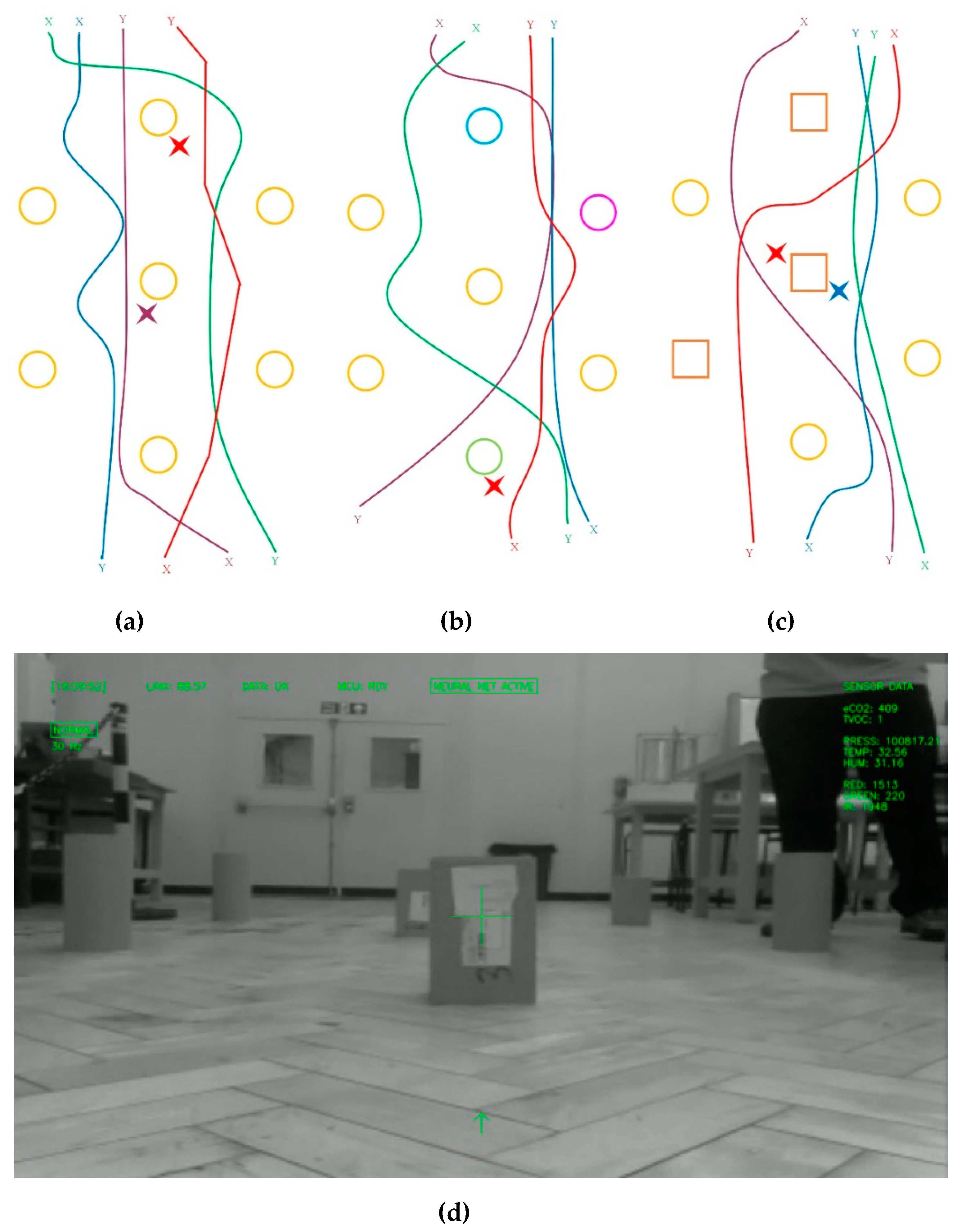
  • The neural network was able to avoid the obstacles and navigate around the obstacle course, predominantly without collisions. The collisions that did occur happened when the course corrections made by the neural network caused the obstacle to go out of the field of view, resulting in the wheel hitting the obstacle.
  • The color obstacle course, in which some of the orange obstacles were replaced with dark and light colors, such as magenta, blue, or green, did not confuse the neural network. When the robot came close to these obstacles, the neural network chose an appropriate directional output to avoid it. As grayscale images were used for inference, this demonstrates that the intensity of obstacles does not matter and the contrast of the object was being recognized.
  • The directional control keys were chosen by the robot in such a way as to keep it within the obstacle course without exiting it, even if no clear bounding walls were provided. This demonstrates that the network appeared to use the obstacles as navigational waypoints to keep the robot within the course and was not just simply demonstrating a collision avoidance random walk. To verify this, the distance between the obstacles at the edges were changed or these edge obstacles were removed completely and the robot was still able to exit the course.
  • The way in which the direction was chosen for avoiding obstacles appears to be based on which side the obstacle lay from the center of the frame. For example, if the obstacle lay to the left of the frame the “forward-right” (W+D key combination) direction was chosen to avoid the obstacle completely. When driving the robot for creating the training dataset, it was not intentionally driven like this, however, a more systematic set of training data was required to see if this was a significant deduction of the neural network.
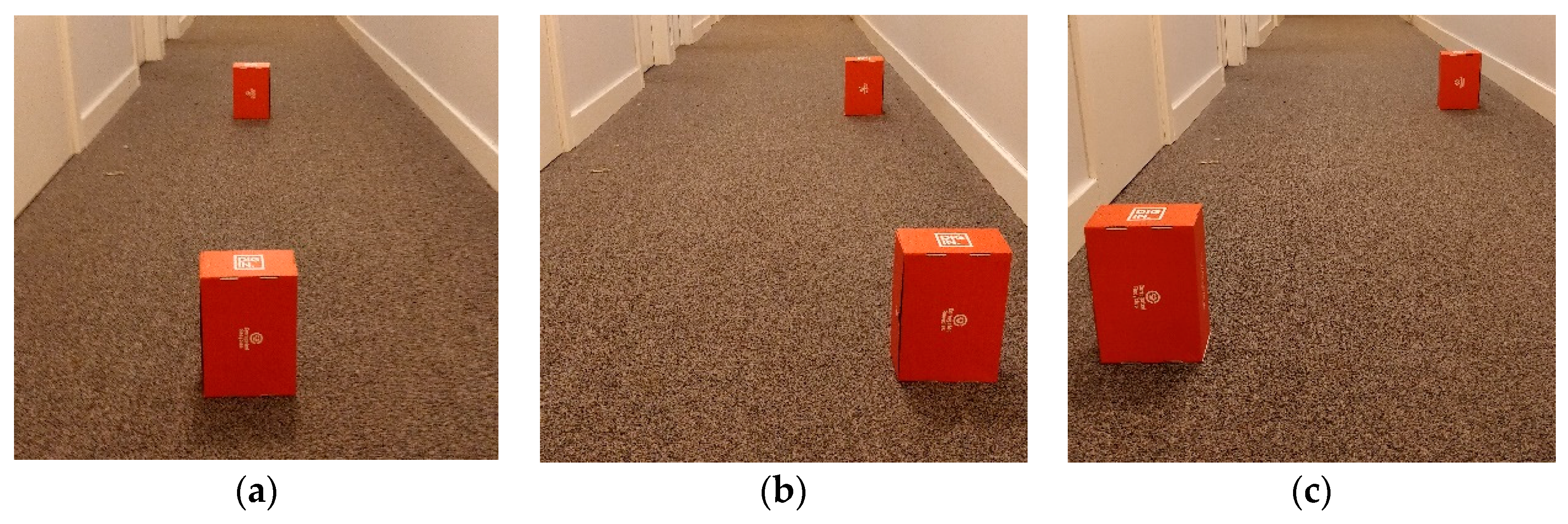
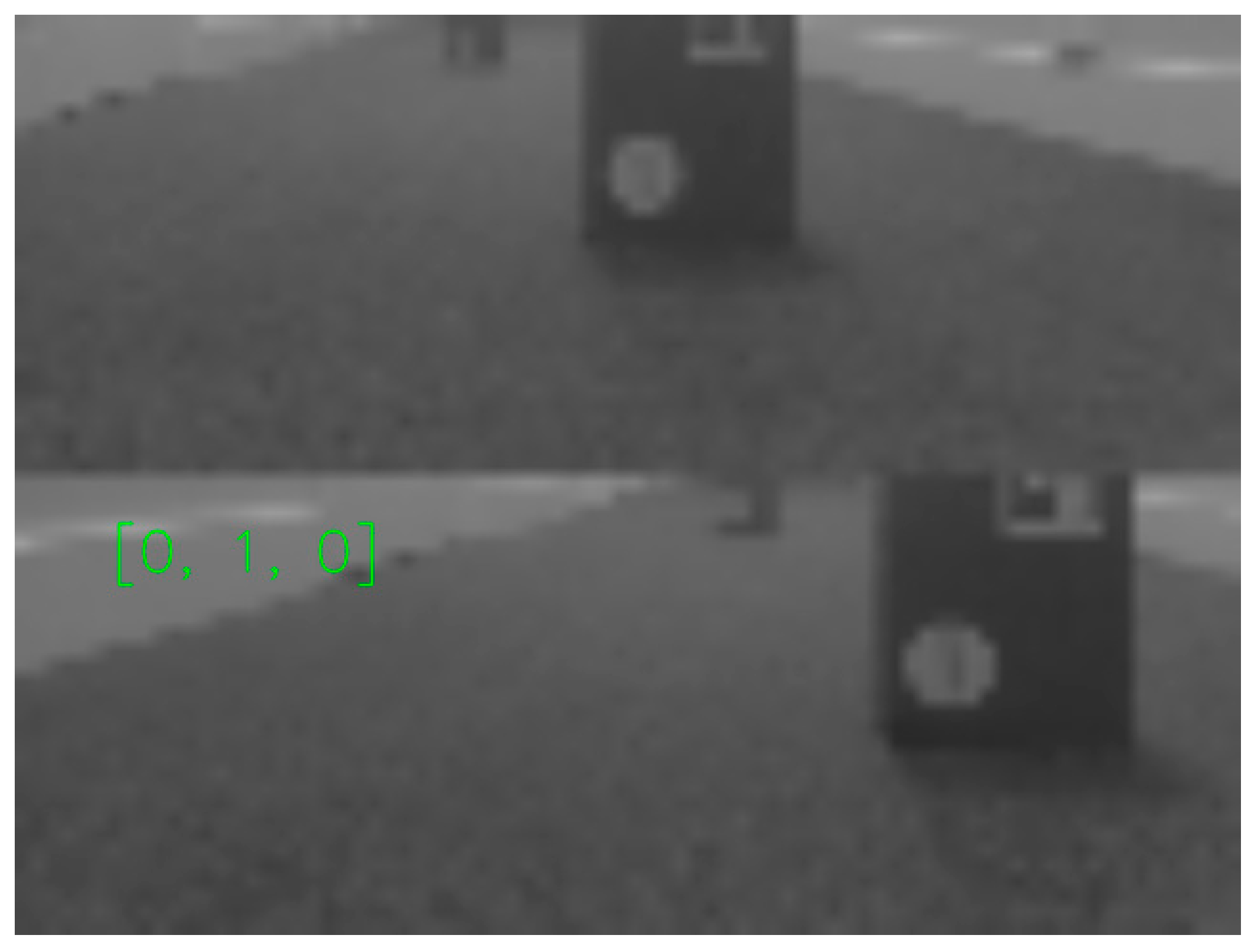
  • When cylindrical obstacles were replaced by box-shaped obstacles (the surface of which contained stickers as shown in Figure 6d), the neural network still recognized them as obstacles and proceeded to navigate around them. Only on a few occasions did collisions occur with the boxes.
  • Although the plots are smooth in Figure 6, in actuality, there was a high level of fluctuation in the way the robot chose the directional control, and as result, the actual trajectory of the robot showed a more pronounced jagged or saw-tooth like pattern. This problem can be associated to the fact that the neural network did not have any memory of the past action or state of the environment.
  • Even when the robot was placed at different starting locations and orientations (but still pointing into the obstacle course), the robot entered the course and completed it successfully.

4.2.2. Gate Test

In this test, the obstacles were placed in such a way that it formed a gate in the middle with a gap of approximately 70 cm, as shown in Figure 7a. Two variations of this were also performed, one with the same arrangement but with different colored cylinders (see Figure 7b), and one where two orange cylinders were laid on their sides to make a gap of approximately 90 cm (see Figure 7c). These types of arrangements were not in the training data and were new to the neural network controller. The expectation would be for the robot to go through the gap without colliding with any of the obstacles. The observations from these tests were:
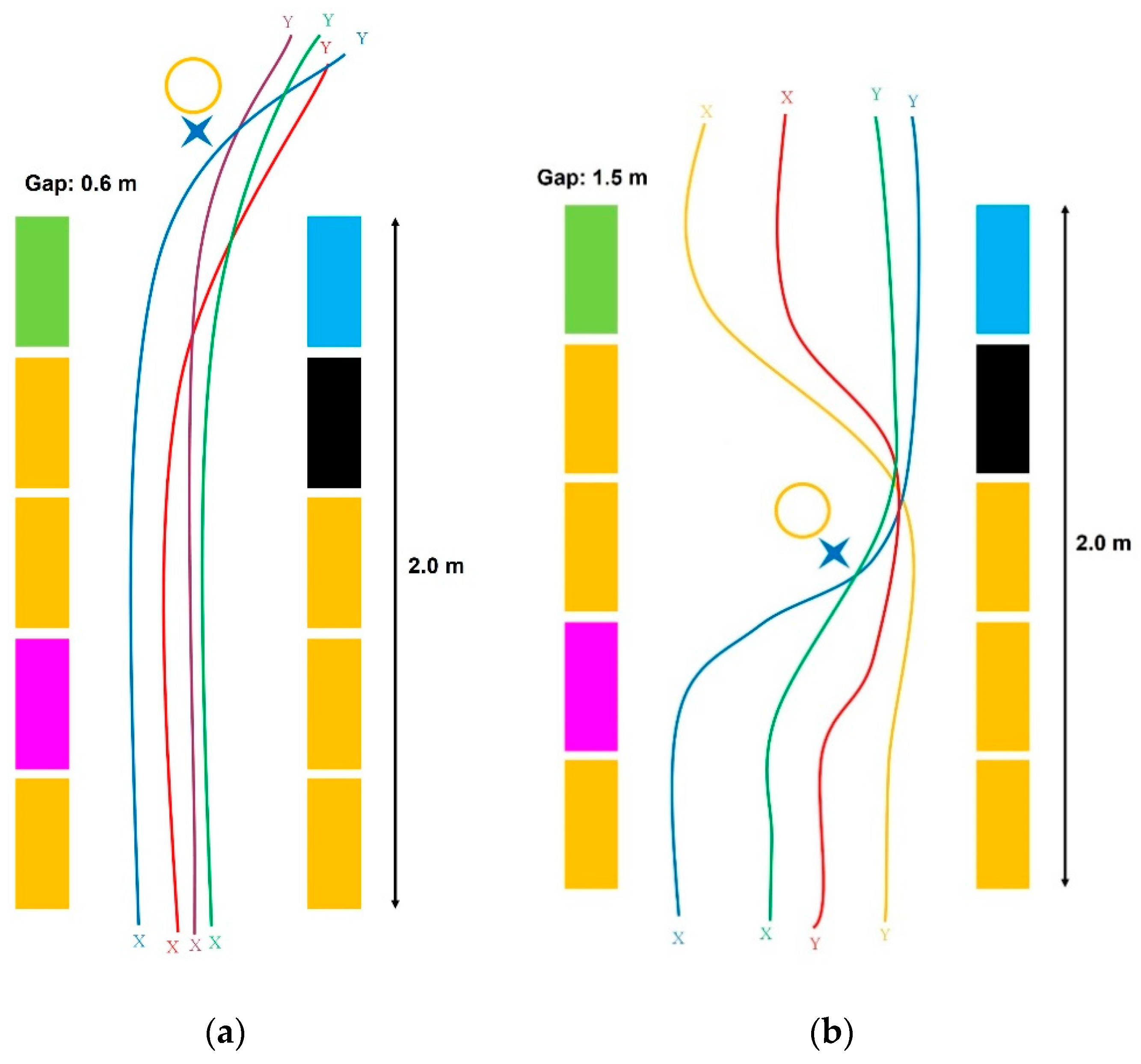
  • The neural network was able to clear the gate most of the time provided that the gate was visible in the frame to some degree. When the robot was either placed with half of the gate showing or at an angle with obstacles and the gate in view, the robot successfully cleared the gate. All of these tests were conducted with a starting distance of at least 1.2 m. If the robot was placed too close to the obstacles, namely at a 0.6 m distance, the neural network failed to use the correct directional control keys, even if the gap came partially into view. This issue was attributed to the limited field of view of the camera.
  • The obstacles were replaced with color ones to confuse the neural network controller but the results were the same as in the case where all the obstacles were orange. Again, if the robot was placed too close to the obstacles initially, a collision occurred.
  • When the obstacles were laid on the ground, the robot managed to pass through the gate. However, on one occasion, the obstacle was seen by the neural network and collision was prevented but the robot veered off to the left and did not pass through the gate. This was probably because the camera had lost sight of the obstacle.

4.2.3. Hallway Test

In the hallway test, the obstacles were laid on the ground as shown in Figure 8. The obstacles on either side were randomly colored as before to see whether the neural network could differentiate this feature. Two variations of the test were performed, one with the obstacle at the end and one with the obstacle placed at the center of the course. The main observations were:
  • The neural network was able to keep the robot between the obstacles on either side even though the colored cylinders were used and this type of environment was not in the dataset. The direction control keys decided by the network still fluctuated, and therefore the actual robot trajectory was jagged and not as smooth as indicated in Figure 8.
  • The obstacle placed at the end of the hallway course was added to provide an additional challenge, but as demonstrated, the robot chose to turn right each time. The exact cause for this remains unknown as the initial training dataset was balanced; the rights were almost equal to the lefts and forwards. It is speculated that some other object in the environment was causing the neural network to preferentially deviate to that side.
  • With the obstacle in the middle of the hallway, the robot negotiated the course on most occasions, but as previously seen, due to losing sight of the obstacle, collisions between the wheel and the cylinder did occasionally occur.

4.2.4. Human Leg Avoidance

As a quick final test, a human leg was used as the obstacle, which the neural network was not trained to avoid. However, the robot still managed to navigate this successfully. This was due to the contrast between the shoe and leg against the background. This result implies that the neural network may have learned to segment the image and be able to differentiate between foreground and background objects.

4.3. Memory Model

As seen in the above tests, most of the collisions that occurred was caused by the correction made by the neural network when the object was out of the frame. This was because the neural network had no memory of the past event. Each new frame was a new world to the neural network that it needed to decide on without the past being remembered. Since the architecture of AlexNet does not have any memory element, a simple solution was considered in which a past frame is stored and the current frame is concatenated with the past, with this combined image then being forwarded through the network. In this way, the network can decide based on a past and current frame and effectively provides a single snapshot memory image to consider.
To do this, the existing dataset of the corridor was used as a test to see whether this solution would work. The dataset was created using the bottom part of a frame at index 1 at a resolution of 80 pixels × 30 pixels, then skipping 10 frames and selecting the bottom part of the image again. The two images were joined together with the old frame set at the top and the new frame set at the bottom. This recreated the image size required for processing by the neural network, an example of which is shown in Figure 9. The process is repeated to create a dataset of approximately 11,500 samples. The training was done for 15 epochs at a learning rate of 0.0001 and achieved an accuracy of 94 percent. This model was used as this was the same configuration that was used in Section 4.1 for the corridor.
When running the neural network on this image format, the input was constructed from the current and previously saved image. Concatenating an image from 10 frames previous at a 20 frames per second rate corresponds to a memory snapshot of 0.5 s ago. Implications of this approach is the memory overhead in needing to store the previous images required for memory, in this case 10 frames. Initial testing of this approach currently indicates no improvement in the performance of the neural network as the network performed similarly to the results shown in Section 4.1.

4.4. Discussion

From the tests, it can be seen that the CNN controller had definitely learned how to navigate an obstacle course using only a single video feed with no purpose-built simulations required to program the network and the results show a comparable performance to previously reported implementations of neural networks on mobile robots [17,18,19,20,21,22,23]. Notable exceptions were that collisions occasionally happened, this being caused by the limited field of view of the camera preventing the robot knowing of an object in close proximity alongside it, and that the current network would also struggle to identify dynamic objects as only single snapshots of time are considered and it would therefore perceive dynamic objects as static ones. Another issue with the current controller was the rapid fluctuations in the predicted trajectory as the network had no memory of the previous action that the robot took. When new frames were given to the network, it considered it as a new environment each time and decided which key it needed to press. A human driver is able to navigate the obstacle course because the driver understands the shape of the robot, keeps in memory that even if the obstacle is not visible, it is still near the robot and therefore continues to move in a way that avoids collision and is able to plan a smooth path. None of these attributes is demonstrated by the CNN controller because this neural network does not understand sequences of events and time. A different architecture is needed that has memory, for example, a convolutional LSTM (long short-term memory) network could be used [34]. In a convolutional LSTM, a CNN network is fitted with an LSTM network at the output and is therefore able to decide actions based on past data. It would therefore be beneficial, not only to account for previously passed static objects, but also trajectories of dynamic objects. For such networks, training must be done with datasets that are sequential.
The results suggest that the network was capable of obstacle identification, where it was using image segmentation to separate out the obstacles from the background. As the color of the obstacle did not matter, this being aided by the fact that the grayscale image was used, the network had learnt the features of an obstacle instead of depending on the color. This could be, for example, edge features or intensity contrasts. It was noted that the robot, after exiting the obstacle course, straightened itself. The CNN controller was possibly using the pattern of the wood tiling used in the floor of the lab to get a sense of orientation. For example, the network may have learned a particular way the floor pattern should look if no obstacles are visible and controlled the robot to achieve the correct floor pattern.
The main change that should be made is to use reinforcement learning instead of supervised learning in which a labeled dataset is needed. The creation of the labeled dataset is a tedious task, but if reinforcement learning, is used the agent will learn the best action that gives the maximum reward; for example, the reward could be considered as keeping a certain distance away from the obstacle and traveling forward. This is one example of how a reward can be provided, but in reality, the problem of reward assignment is challenging. Another problem with reinforcement learning is that it requires trial and error of actually driving the robot around, letting the agent make mistakes and learning from it. This is problematic to do in a real environment because of the resulting damage that may occur. To solve this issue, a simulation is normally used where the agent is allowed to make as many mistakes as it wants. A recent paper by Ha and Schmidhuber [35] called World Models provides a possible solution to this. In this, the authors used reinforcement learning to train a network to drive a car in a top down racing game. A variational autoencoder (VAE) [36] was used to recreate the environment with slight variations and an LSTM network provided information on how the environment evolved after the agent took an action in the virtual world. Once the network learned how to control the car in this virtual world, it was able to successfully control the car in the racing game. An adaption of this technique can be used for FumeBot, in which the robot is able to look at the environment, create a virtual version, and then execute actions in it. Once a good set of controls is achieved, it is then transferred to the real environment and appropriate actions are executed. The challenge to do the above is creating an appropriate reward mechanism in this virtual environment.
An issue faced in this project was the limited amount of memory available for the network. Although circumvented here, this would be problematic if the approach used in the World Model paper was directly used on a real environment as compared to the relatively simpler 2D racing game due to the detail and complexity required. To make the above model work in a real environment, a neural Turing machine (NTM) [37] can be used, in which the memory is separated from the neural network. In this, the DNN learns to interact with a separate memory and is able to learn small algorithms for it. The NTM can also learn longer time steps compared to the LSTM that was used by the authors of World Model. The World Model combined with an NTM could be used for simulating a virtual version of the real environment observed by the robot and train it in that neural network simulation. The NTM also provides the opportunity to learn more complex or multiple tasks when combined with reinforcement learning.

5. Conclusions

The aim of the FumeBot project was to design a deep-neural-network-controlled robot for environmental monitoring. A robotic platform was developed with a range of sensors and cameras with data being streamed wirelessly to a laptop. The GUI application running on the laptop allowed for data monitoring and control of the robot and was also used for interfacing with the convolutional neural network controller for the robot. The CNN controller was used for the navigation of the robot and was trained using a supervised learning technique through the camera feed and directional controls given to the robot. The trained neural network was tested in an obstacle course to see how it was able to perform. The CNN achieved a reasonably good generalization of the task, such that when provided with situations that were not in the dataset, it was still able to complete the required tasks. Incorporating memory capability into the network was identified as the next development to overcome the current limitations in the system. This project also provides a platform to test for new neural network architecture for mobile robots.

Supplementary Materials

Source code used in this project is open source, along with the computer aided design (CAD) files and electrical schematics for the robot, which are available on GitHub at https://github.com/ajithcodesit/FumeBot.

Author Contributions

Conceptualization, A.T. and J.H.; methodology, A.T.; software, A.T.; validation, A.T.; investigation, A.T.; writing—original draft preparation, A.T.; writing—review and editing, J.H.; supervision, J.H.

Funding

This research received no external funding.

Acknowledgments

The authors wish to thank P. Watson, P. Harrison, and F. Atkinson at Newcastle University in assisting with construction of the robot.

Conflicts of Interest

The authors declare no conflict of interest.

Appendix A. Designing Fumebot

Appendix A.1. Chassis

The mechanical design for this prototype robot was kept quite straight forward, allowing enough space for all the electronics, accessibility for quick modification, and space for additional equipment if necessary. A CAD render of the robot is shown in Figure A1a. It has dimensions of 400 mm × 357 mm × 216 mm. The robot utilized a differential drive arrangement, the kinematic model of which was [38]:
φ 1 ˙ = 1 r ( x ˙ + l θ ˙ ) ; φ 2 ˙ = 1 r ( x ˙ l θ ˙ ) ,
where r is the radius of the wheel in meters (m), φ ˙ 1 and φ ˙ 2 are the angular velocity of the left and right wheel, respectively, in radians per seconds (rad/s), l is the half-axle length in m, x ˙ is the x-component of the velocity of the robot in m/s, y ˙ is the y-component of the velocity of the robot (m/s), and θ ˙ is the angular velocity of the rotation of the robot about the z-axis in rad/s. To assist in the training of the network, the robot motion was discretized into eight basic categories, as shown in Figure A1b. The angular velocity of the wheels in rad/s was converted into rpm and was then used to calculate the step frequency to drive the stepper motors at the correct speed. If the rpm of any of the two wheels exceeded the maximum set in the firmware, then the rpm of that wheel was set to the maximum value and the rpm for the other wheel was automatically scaled.
The robot was controlled by an Arduino Mega 2560 microcontroller (Rapid Electronics Limited, Colchester, UK) and a Raspberry Pi 3 Model B (Premier Farnell, Leeds, UK) single board computer (SBC), which was connected to a laptop by a wireless network on which the controlling neural network was being run. The robot used stepper motors for locomotion, which were arranged in a differential configuration and were controlled by the Arduino using commands from the Raspberry Pi. These motors are good for environments where there might be flammable gases present. The stepper motors used for this project were NEMA 17 bipolar stepper motors (17HS19-0854S, OMC Corporation Limited, Nanjing City, China), which run on 5.3 V at 0.85 A per phase. To drive each stepper motor, a Pololu DRV8834 (Hobbytronics Limited, York, UK) was used. Sixteen-bit timers in the Arduino MEGA 2560 were used to control the step frequency and hence control the rpm of the wheels. The motors were powered using an Anker PowerCore 20,100 (Amazon, Seattle, WA, US) battery bank. A separate battery bank was used to power the remaining electronics. The robot was able to stay mobile for at least 2.5 h using these banks. The main parameters used for the robot are summarized in Table A1.
Figure A1. (a) Render of the FumeBot prototype, and (b) basic directions the robot can move in.
Robotics 08 00062 g0a1
Table A1. Main design parameters for FumeBot.
ParametersMinimumTypicalMaximum
Half axle (l)-166 mm-
Wheel radius (r)-70 mm-
Movement   speed   ( x ˙ ) 10.20 ms−1-0.30 ms−1
Turn   speed   ( θ ˙ ) 145°s−1-75°s−1
Turn radius (R) 2-332 mm-
Stepper motor allowed speed 127 rpm-41 rpm
Steps done per command-50 steps-
1 The speed range was limited to prevent skipping of steps when driving the motors. 2 Defined value for curved motion.

Appendix A.2. Sensors and Communications

The robot is fitted with several environmental sensors and two cameras. The sensor array can be expanded to suit the application needs without too much hassle when it comes to changing the firmware of the microcontroller. The main sensors the robot currently has are:
  • a MAX30105 particle sensor (Mouser Electronics, Mansfield, TX, US) used to detect smoke particles in the atmosphere, a CCS811 metal oxide (MOX) gas sensor (Mouser Electronics, Mansfield, TX, USA) used to detect the presence of equivalent carbon dioxide (eCO2) and total volatile organic compounds (TVOC) in the atmosphere, and a BME280 environmental sensor (Mouser Electronics, Mansfield, TX, USA) used to determine temperature, pressure, and relative humidity readings. The data from the BME280 is also used to compensate the CCS811 sensor. All these sensors are connected to an Arduino and use the I2C (inter-integrated circuit) bus for communication.
  • a FLIR Lepton 3 camera (Digi-Key Corporation, Thief River Falls, MN, USA) provides a thermal view of the environment. Communication is via SPI (serial peripheral interface) to the Raspberry Pi at 9 frames per second and a resolution of 160 pixels by 120 pixels. In principle, this camera could be used as the data stream for the neural network; however, in practice, it was found that communication with this device was lost after 5 to 10 min of operation due to the loss of synchronization. It was therefore only used to provide snapshots of the environment rather than a continuous video stream.
  • a Raspberry Pi Camera v1.3 (The Pi Hut, Haverhill, UK) provides a visible view of the environment. The camera is connected to the Raspberry Pi using a CSI (camera serial interface) and with a 5 MP resolution at 30 Hz, the video quality is acceptable for this application. Ultimately, this data is processed on a laptop and therefore, to prevent problems with video feed lags, the raw image data was converted to JPEG format before transmission.
The camera mount for the robot was placed at the front center, and the mount was capable of panning and tilting via two Tower Pro SG90 micro servo motors (Rapid Electronics Limited, Colchester, UK). To avoid vibrations of the tilt assembly caused by the robot’s movement, the fork assembly onto which the tilt assembly was mounted was supported by three bearings that also took some of the load away from the pan servo motor. This made the camera frames less blurry during movement. The normal optical camera and thermal camera were mounted at exactly the center of the robot on the tilt assembly so the view when the camera was facing forwards was balanced.
A schematic of the connectivity of the various subsystems is shown in Figure A2. The laptop acted as the server where the neural network runs and was used for navigation of the robot using the image frames sent from it. The Raspberry Pi acted as the main controller for the robot and performed the heavy computational tasks like image compression and also handled the communications aspect of the robot. Raspberry Pi to Arduino communication was via the universal asynchronous receiver transmitter (UART) with the appropriate 5 V to 3.3 V signal level shifting. The Arduino microcontroller was responsible for low level tasks like interfacing with sensor and drivers. The communication between the Raspberry Pi and the laptop should be wireless, and therefore Wi-Fi was chosen since both the devices supported this communication method. To make use of the Wi-Fi communication, the sockets library that comes standard with Python was used. The laptop acted as the server and the Raspberry as the client. At this point, a GUI application became necessary on the server side since many controls were required, for example, input area to change the internet protocol (IP) address, ports for the wireless connection, a button to start the connection, and a display area for the frames coming from the camera. A GUI application was written to be run on the laptop using Python bindings for Qt4 and sockets in the Python programming language. The socket was set up to use transmission control protocol (TCP)/IP and had to be threaded since the function of the sockets library were of the blocking types, and as a result, could not be used directly in the GUI program as it would hang when sending or receiving data. A similar program was written for the Raspberry Pi side by using sockets and Python to enable communication with the server. Both of the programs have the ability to send and receive data. The structure of the client (Raspberry Pi side) is shown in Figure A3. The client-side program made use of socket and serial libraries in Python.
Figure A2. Overall communication structure of the robot utilizing transmission control protocol/internet protocol (TCP)/IP, camera serial interface (CSI), serial peripheral interface (SPI), universal asynchronous receiver-transmitter (UART), and inter-integrated circuit bus (I2C).
Robotics 08 00062 g0a2
Figure A3. Structure of Raspberry Pi side program.
Robotics 08 00062 g0a3
As a backup communication method for when Wi-Fi is not available, an Adafruit FONA 3G (Rapid Electronics Limited, Colchester, UK) cellular module using the SIMCom SIM5320A chip, a GSM/cellular quad-band antenna (The Pi Hut, Haverhill, UK), and a subscriber identity module (SIM) card was installed on the robot. The module was successfully tested by sending an SMS text alert to a mobile phone when the gas or particle sensor thresholds were reached. Although such back up communication options are necessary for applications involving automated monitoring, it was not required for the work presented here.

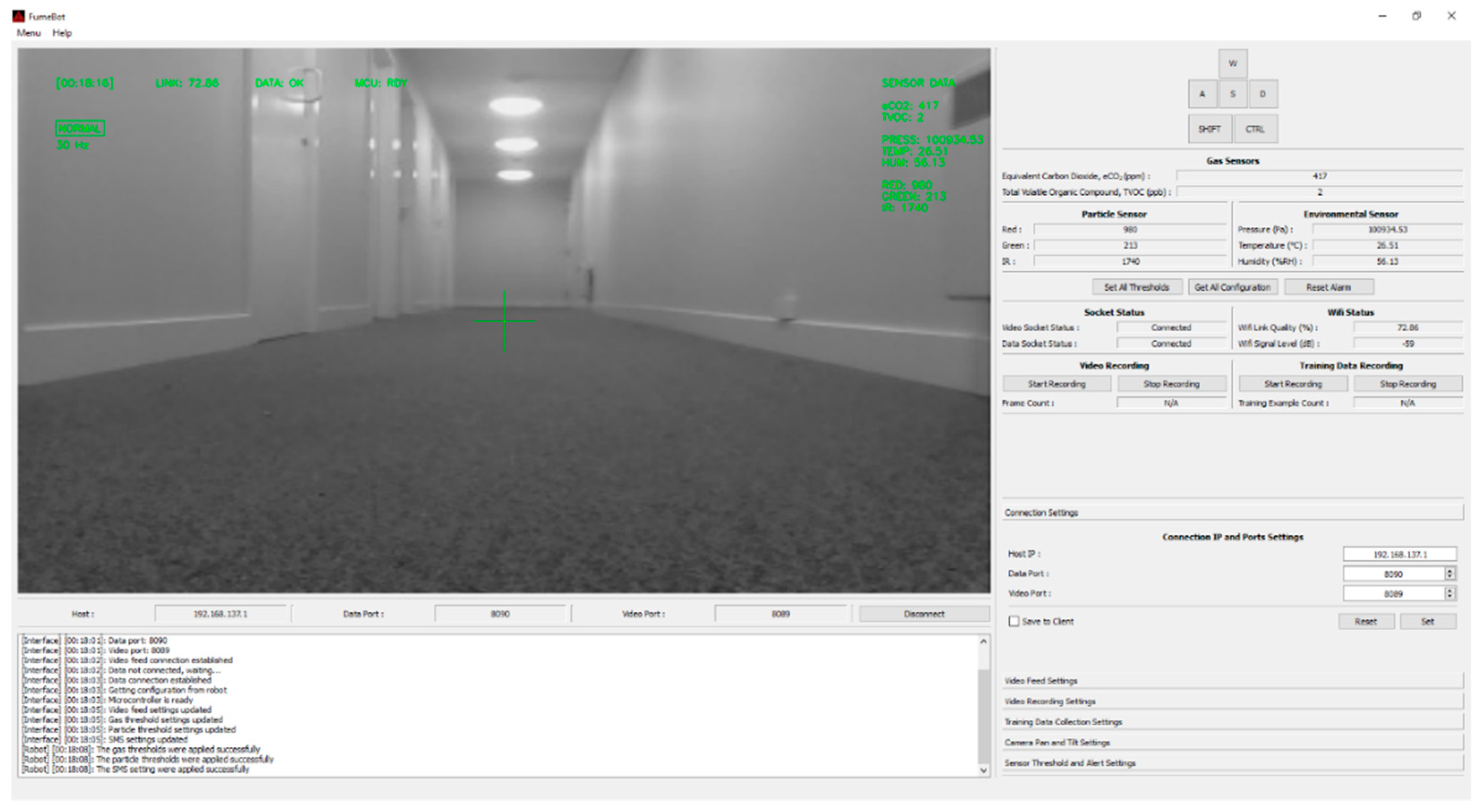
Appendix A.3. Graphical User Interface for FumeBot

The graphical user interface (GUI) shown in Figure A4 has all the features to control the robot, receive and display data coming from the robot’s sensors, displaying the normal optical and thermal camera frames, checking connection statuses, and collecting training data for the neural network. The GUI was made with the help of Qt designer for making the skeleton GUI, PyQt4 (a Python binding for the Qt4 GUI building framework), OpenCV used for computer vision, sockets for communication via TCP/IP using Wi-Fi, Numpy for array manipulation, and other standard libraries in Python.
Figure A4. FumeBot graphical user interface application.
Robotics 08 00062 g0a4
A brief description of the features and settings available to the user are discussed below.
  • The video display area can be toggled to display the images coming from the optical or thermal camera or a blended image of both. A head-up-display is used to display relevant information directly on top of the video frame to avoid looking away from the video display area. For panning and tilting the camera mount, the mouse is dragged across the video display area while holding down the left mouse button.
  • The keyboard is used to control the movement of the robot using the WASD keys while the shift and control keys are used for increasing the speed and braking, respectively.
  • The connection settings are used to change the IP address and ports that are used to communicate with the robot. These settings are also saved to the Raspberry Pi.
  • The sensors tab contains all the alert thresholds for the gas and particle sensors. The SMS settings for text alerts are also available here.
  • The video feed settings tab provides control for image size, frame rate, and color settings. For the capture color, grayscale is preferred as the amount of data that needs to be sent after JPEG compression is considerably less when compared to color frames.
  • The video recording and training data settings tabs are used to record the video feed frames coming from the robot. The video files are recorded with time stamps so each new recording creates a new file. The training data consists of the image frame coming from the normal optical camera of the robot and the WASD key presses to move the robot. Only the optical camera data is collected because of the issues with the thermal camera, as explained above.
For collecting the training data, if any of the keys used to control the movement of the robot are pressed, the video frame that is being currently displayed and the key press is saved to a list. When the user has collected the required amount of data and stops the recording, the list is converted to a Numpy array and then saved to the specified location under the preset name. The training data is saved in to two files, one is the training dataset Numpy file with the “npy” extension and the other is the meta file, which is used to store the configurations used to collect the training data with the “.meta” extension. The meta file contains the file name of the training dataset associated with it and the key order. This way of saving the configuration in a separate file was required because the Numpy library does not have built in support for including meta information.
The training data recording is started either by pressing the T key or by using the GUI buttons. If the GUI is used, the recording can be paused so unwanted key presses when reorienting the robot will not be collected. The neural network is activated or deactivated by pressing the N key or the provided GUI button. The decision made by the neural network is processed by the GUI application and the commands for movement are sent to the robot.

References

  1. Roomba Robot Models. Available online: https://www.irobot.co.uk/home-robots/vacuuming (accessed on 18 July 2019).
  2. Dyson 360 Eye robot. Available online: https://www.dyson.co.uk/robot-vacuums/dyson-360-eye-overview.html (accessed on 18 July 2019).
  3. Bosch Indego. Available online: https://www.bosch-garden.com/gb/en/garden-tools/garden-tools/robotic-lawnmowers-209530.jsp (accessed on 18 July 2019).
  4. Flymo Robot Lawn Mowers. Available online: https://www.flymo.com/uk/products/robot-lawn-mowers/ (accessed on 18 July 2019).
  5. Wilson, G.; Pereyda, C.; Raghunath, N.; de la Cruz, G.; Goel, S.; Nesaei, S.; Minor, B.; Schmitter-Edgecombe, M.; Taylor, M.E.; Cook, D.J. Robot-enabled support of daily activities in smart home environments. Cogn. Syst. Res. 2019, 54, 258–272. [Google Scholar] [CrossRef]
  6. Marek, G.; Peter, S. Design the robot as security system in the home. Procedia Eng. 2014, 96, 126–130. [Google Scholar] [CrossRef]
  7. Song, G.; Yin, K.; Zhou, Y.; Cheng, X. A Surveillance Robot with Hopping Capabilities for Home Security. IEEE Trans. Consum. Electron. 2009, 55, 2034–2039. [Google Scholar] [CrossRef]
  8. Di Paola, D.; Milella, A.; Cicirelli, G.; Distante, A. An Autonomous Mobile Robotic System for Surveillance of Indoor Environments. Int. J. Adv. Robot. Syst. 2010, 7, 19–26. [Google Scholar] [CrossRef]
  9. Tseng, C.C.; Lin, C.L.; Shih, B.Y.; Chen, C.Y. SIP-enabled Surveillance Patrol Robot. Robot. Comput. Integr. Manuf. 2013, 29, 394–399. [Google Scholar] [CrossRef]
  10. Liao, Y.L.; Su, K.L. Multi-robot-based intelligent security system. Artif. Life Robot. 2011, 16, 137–141. [Google Scholar] [CrossRef]
  11. Ahn, H.S.; Sa, I.K.; Choi, J.Y. PDA-Based Mobile Robot System with Remote Monitoring for Home Environment. IEEE Trans. Consum. Electron. 2009, 55, 1487–1495. [Google Scholar] [CrossRef]
  12. Redmon, J.; Divvala, S.; Farhadi, A. You Only Look Once: Unified, Real-Time Object Detection. Comput. Vis. Pattern Recognit. 2015, arXiv:1506.02640. [Google Scholar]
  13. He, K.; Gkioxari, G.; Dollár, P.; Girshick, R. Mask R-CNN. Comput. Vis. Pattern Recognit. 2017, arXiv:1703.06870. [Google Scholar]
  14. Hannun, A.; Case, C.; Casper, J.; Catanzaro, B.; Diamoz, G.; Elsen, E.; Prenger, R.; Satheesh, S.; Sengupta, S.; Coates, A.; et al. Deep Speech: Scaling up end-to-end speech recognition. Comput. Lang. 2014, arXiv:1412.5567. [Google Scholar]
  15. Oord, A.; Dieleman, S.; Zen, H.; Simonyan, K.; Vinyals, O.; Graves, A.; Kalchbrenner, N.; Senior, A.; Kavukcuoglu, K. WaveNet: A Generative Model for Raw Audio. Sound Mach. Learn. 2016, arXiv:1609.03499. [Google Scholar]
  16. Fridman, L.; Brown, D.E.; Glazer, M.; Angell, W.; Dodd, S.; Jenik, B.; Terwilliger, J.; Patsekin, A.; Kindelsberger, J.; Ding, L.; et al. MIT Autonomous Vehicle Technology Study: Large-Scale Deep Learning Based Analysis of Driver Behavior and Interaction with Automation. Comput. Soc. 2017, arXiv:1711.06976. [Google Scholar]
  17. Janglová, D. Neural Networks in Mobile Robot Motion. Int. J. Adv. Robot. Syst. 2004, 1, 15–22. [Google Scholar] [CrossRef]
  18. Parhi, D.R.; Singh, M.K. Real-time navigational control of mobile robots using an artificial neural network. Proc. Inst. Mech. Eng. Part. C J. 2009, 223, 1713–1725. [Google Scholar] [CrossRef]
  19. Shamsfakhr, F.; Sadeghibigham, B. A neural network approach to navigation of a mobile robot and obstacle avoidance in dynamic and unknown environments. Turk. J. Electr. Eng. Comput. Sci 2017, 25, 1629–1642. [Google Scholar] [CrossRef]
  20. Chi, K.H.; Lee, M.F.R. Obstacle avoidance in mobile robot using neural network. In Proceedings of the International Conference on Consumer Electronics, Communications and Networks, Xianning, China, 16–18 April 2011; pp. 5082–5085. [Google Scholar]
  21. Takiguchi, T.; Lee, J.H.; Okamoto, S. Collision avoidance algorithm using deep learning type artificial intelligence for a mobile robot. In Proceedings of the International Multi Conference of Engineers and Computer Scientists, Hong Kong, China, 14–16 March 2018. [Google Scholar]
  22. Wu, K.; Esfahani, M.A.; Yuan, S.; Wang, H. Learn to Steer through Deep Reinforcement Learning. Sensors 2018, 18, 3650. [Google Scholar] [CrossRef]
  23. Xie, L.; Wang, S.; Markham, A.; Trigoni, N. Towards Monocular Vision based Obstacle Avoidance through Deep Reinforcement Learning. Robotics 2017, arXiv:1706.09829. [Google Scholar]
  24. Yang, S.; Konam, S.; Ma, C.; Rosenthal, S.; Veloso, M.; Scherer, S. Obstacle avoidance through deep networks based intermediate perception. Robotics 2017, arXiv:1704.08759. [Google Scholar]
  25. Singla, A.; Padakandla, S.; Bhatnagar, S. Memory-based deep reinforcement learning for obstacle avoidance in UAV with limited environment knowledge. Robotics 2018, arXiv:1811.03307. [Google Scholar]
  26. Hwu, T.; Isbell, J.; Oros, N.; Krichmar, J. A self-driving robot using deep convolutional neural networks on neuromorphic hardware. Neural Evol. Comput. 2016, arXiv:1611.01235. [Google Scholar]
  27. Hinton, G.E.; Srivastava, N.; Krizhevsky, A.; Sutskever, I.; Salakhutdinov, R.R. Improving neural networks by preventing co-adaptation of feature detectors. Neural Evol. Comput. 2012, arXiv:1207.0580. [Google Scholar]
  28. Bengio, Y. Practical recommendations for Gradient-Based training of deep architectures. Learning 2012, arXiv:1206.5533v2. [Google Scholar]
  29. Krizhevsky, A.; Sutskever, I.; Hinton, G.E. ImageNet classification with deep convolutional neural networks. Adv. Neural Inf. Process. Syst. 2012, 25, 1097–1105. [Google Scholar] [CrossRef]
  30. Nair, V.; Hinton, G.E. Rectified linear units improve restricted Boltzmann machines. In Proceedings of the 27th International Conference on Machine Learning (ICML-10), Haifa, Israel, 21–24 June 2010; pp. 807–814. [Google Scholar]
  31. LeCun, Y.; Bottou, L. Efficient BackProp. Neural Networks: Tricks of the Trade; Orr, G.B., Müller, K.R., Eds.; Springer-Verlag: Berlin/Heidelberg, Germany, 1998; pp. 9–50. [Google Scholar]
  32. CS231n Convolutional Neural Networks for Visual Recognition. Available online: http://cs231n.github.io (accessed on 11 June 2019).
  33. Kingma, D.P.; Ba, J. Adam: A Method for Stochastic Optimization. In Proceedings of the 3rd International Conference for Learning Representations, San Diego, CA, USA, 7–9 May 2015. [Google Scholar]
  34. Hochreiter, S.; Schmidhuber, J. Long Short-Term Memory. Neural Comput. 1997, 9, 1735–1780. [Google Scholar] [CrossRef]
  35. Ha, D.; Schmidhuber, J. World Model. Mach. Learn. 2018, arXiv:1803.10122. [Google Scholar]
  36. Kingma, D.P.; Welling, M. Auto-Encoding Variational Bayes. Mach. Learn. 2014, arXiv:1312.6114. [Google Scholar]
  37. Graves, A.; Wayne, G.; Danihelka, I. Neural Turing Machines. Neural Evol. Comput. 2014, arXiv:1410.5401. [Google Scholar]
  38. Siegwart, R.; Nourbakhsh, I.R. Introduction to Autonomous Mobile Robots, 1st ed.; MIT Press: Cambridge, MA, USA, 2004; pp. 51–52. [Google Scholar]
Figure 1. Final CNN layer stacking.
Robotics 08 00062 g001
Figure 2. Prototype of FumeBot. For the purposes of this development phase of the robot, the robot chassis was simply rapid-prototyped out of laser cut plywood.
Robotics 08 00062 g002
Figure 3. AlexNet for FumeBot.
Robotics 08 00062 g003
Figure 4. Various scenarios for the corridor obstacle test with boxes being (a) centered, (b) off-center to one side, and (c) off-center both sides.
Robotics 08 00062 g004
Figure 5. (a) The lab obstacle course, and (b) corresponding dimensions for this course.
Robotics 08 00062 g005
Figure 6. (a) The course used to train and test the neural network, where positions X and Y correspond to the start and end positions, respectively; (b) variation of (a) with different-colored obstacles used for testing; (c) variation of (a) with different-shaped/looking obstacles used for testing; (d) captured image showing the different appearance of the obstacles used in (c).
Robotics 08 00062 g006
Figure 7. (a) Results for the basic gate test, where positions X and Y correspond to the start and end positions, respectively; (b) results for the color gate test; and (c) results for the lying obstacle gate test.
Robotics 08 00062 g007
Figure 8. (a) Results for the tunnel test with an obstacle positioned at the end, where positions X and Y correspond to the start and end positions, respectively; and (b) results for the tunnel test with an obstacle positioned at the middle of the course.
Robotics 08 00062 g008
Figure 9. An example of a concatenated image for assessing a memory model approach. The image consists of an old image (top half) and the current image (bottom half). The directional input for this frame combination is highlighted in green in the figure.
Robotics 08 00062 g009
Table 1. CNN training results for the corridor dataset.
Model NumberLearning RateEpochsTest Accuracy
10.00011293
20.00011595
30.00012096
40.00014096
Table 2. CNN training results for the lab dataset.
Model NumberLearning RateEpochsAccuracy
10.00011295
20.00011595
30.00012096
40.00014097

