A Sensor-Network-Supported Mobile-Agent-Search Strategy for Wilderness Rescue

Abstract

Mobile target search is a problem pertinent to a variety of applications, including wilderness search and rescue. This paper proposes a hybrid approach for target search utilizing a team of mobile agents supported by a network of static sensors. The approach is novel in that the mobile agents deploy the sensors at optimized times and locations while they themselves travel along their respective optimized search trajectories. In the proposed approach, mobile-agent trajectories are first planned to maximize the likelihood of target detection. The deployment of the static-sensor network is subsequently planned. Namely, deployment locations and times are optimized while being constrained by the already planned mobile-agent trajectories. The latter optimization problem, as formulated and solved herein, aims to minimize an overall network-deployment error. This overall error comprises three main components, each quantifying a deviation from one of three main objectives the network aims to achieve: (i) maintaining directional unbiasedness in target-motion consideration, (ii) maintaining unbiasedness in temporal search-effort distribution, and, (iii) maximizing the likelihood of target detection. We solve this unique optimization problem using an iterative heuristic-based algorithm with random starts. The proposed hybrid search strategy was validated through the extensive simulations presented in this paper. Furthermore, its performance was evaluated with respect to an alternative hybrid search strategy, where it either outperformed or performed comparably depending on the search resources available.

1. Introduction

Many real-world problems can be formulated as a mobile-target search problem, including those used to locate lost persons [1,2,3,4,5,6,7,8]. These problems often involve searching for an un-trackable target whose location is unknown in real-time for the entire duration of the search. Planning such a search, typically, necessitates the coordination of resources to maximize the probability of successful target detection [9,10,11,12]. The work presented in this paper, for example, considers the problem of planning a search to locate a (mobile) target with a team of mobile agents supported by a static-sensor network. Namely, it considers planning the best achievable sensor network to be deployed by a team of mobile agents whose motion trajectories have already been predetermined (i.e., which can drop sensors only along their paths), as shown in Figure 1.

Earlier solutions to this problem have focused on using solely mobile agents [12,13,14,15,16,17,18,19,20,21,22,23,24,25,26]. For example, in reference [22], a formation-based search method is presented. The proposed method ensures that searchers always maintain complete coverage along their sweep. In reference [23], a method for dynamic reconfiguration of the search space is presented. The method allows unmanned aerial vehicles (UAVs) to continue tracking targets even after it moves beyond the initial search area boundaries. In reference [24], Bayesian estimation is suggested to estimate and update the target’s location likelihood for search with UAVs. The recursively updated target-location likelihood is, then, used to guide the search.

Static-sensor networks have also been proposed for search and surveillance applications [27,28,29,30,31,32,33]. These, however, have not explicitly considered dynamic scenarios where the target-location likelihood function can change over time and that the search area may expand with time. A modified approach, dealing with these two issues, was proposed in references [34,35], wherein a static-sensor network is deployed in a time-phased manner.

Hybrid approaches that make use of both static and mobile search resources have also been investigated [36,37,38,39,40,41,42,43]. For example, in reference [37], mobile agents supplement a static-sensor network by patrolling uncovered areas. In [38,39,40], a static-sensor network is maintained by a set of mobile service agents. In reference [41], data is ferried from static-sensor positions to a central location by mobile agents, to address the lack of wireless connectivity in some sensor-deployment scenarios.

In general, the above works do not consider dynamic scenarios in which the region of interest may change and only utilize one of the two available search resources for performing the actual search. For time-critical applications, such as the mobile-target search problem, however, all search resources should be utilized to maximize the probability of successful target detection. Furthermore, past work has typically taken a sensor-centric approach to sensor network planning and deployment. Namely, the network- and delivery-planning problems have been addressed separately, assuming that a network is planned first, and delivery occurs to satisfy it. As such, network planning, typically, takes place without considering whether the deployment is feasible. Similarly, delivery planning occurs assuming the network deployment plan already exists. Past works have also not considered time-phased sensor deployments (i.e., sensors have both scheduled deployments time as well as a specified deployment locations). The addition of such a temporal dimension in sensor-network topology and delivery planning problems can significantly increase its difficulty and complexity. In particular, it introduces the possibility of late sensor deployments, which can compromise the optimality of the sensor network being deployed. This is, especially, true when the number of sensors to deploy is much larger than the number of mobile agents available to deploy them.

Outside of search and rescue applications, other works have focused on the design of multi-agent systems operating in dynamic environments for effective operation at different time scales. In reference [44], results have shown that dynamic changes to a multi-agent network are critical to efficient collective performance at various time scales. Other works have investigated the group controllability of multi-agent systems in dynamic environments for real-time applications [45,46].

In the agent-centric search-planning approach proposed in this paper, mobile agents “drop” static sensors optimally as they follow their respective optimal search trajectories. This approach was taken to eliminate concerns with infeasible ideal sensor-network planning that occur in sensor-centric approaches to network planning and deployment. Namely, the method first plans optimal agent-motion trajectories, followed by planning optimal sensor-deployment positions and times on these trajectories, while maximizing the likelihood of mobile-target detection in an unbounded environment. Our previous work presented a method for optimal agent search planning [21]. In this paper, we extend the approach by developing a novel solution to the latter sensor-deployment optimization problem. One may note that the proposed method takes an optimization-based approach to both agent motion-trajectory planning and sensor-deployment planning. The method, thus, yields an overall plan that is optimal in that it optimizes a reward function defined as part of the method. Due to computational time constraints dictated by the search scenario, however, the proposed approach yields only a near-optimal solution. One may note that the solution could be improved upon with more computational time, reaching a global-optimal solution at the limit.

The proposed hybrid approach is novel in that it guarantees the deployment of a near-optimal static-sensor network, without interfering in the search of a target utilizing a team of mobile agents following their respective optimal trajectories. It additionally guarantees that the sensor deployment will be deployed as planned. The focus of this paper is to develop and present the solution of the latter constrained problem involving the deployment of the static-sensor network for effective target search.

While, the proposed method presented is primarily formulated as one for wilderness search and rescue (WiSAR), where the objective is to locate a lost person as soon as possible [19,47,48,49], it can be adapted to any mobile-target search problem, where the target location likelihood can change during the search and the space-time scales are similar. The search and planning strategy is also generalizable to any other performance measure. Examples of such problems include: urban search and rescue [50,51,52,53,54], target pursuit [55,56], wildlife search [57], and surveillance [58].

2. The WiSAR Planning Problem

The problem addressed in this paper is one of planning a hybrid search to locate a lost person in the wilderness. The search resources include $k$ agents and $n$ static sensors deployed by the agents.

2.1. Search Scenario and Assumptions

A WiSAR scenario, typically, starts with a notification of a missing target. At this point, target demographics and the time and location the target was last seen, herein referred to as the target’s last known position (LKP), are provided to the search team. Although, information regarding how the target is moving is generally not known, it can be inferred using demographic information to develop a probabilistic target motion model [59]. The motion model used in this paper generates target trajectories that consist of series of straight-line segments of varying lengths and headings. This is achieved by specifying a random sequence of headings and distances to travel along each heading. Two parameters are used in the model to specify the characteristics of the motion: the degree of wandering, ${\sigma }_{\theta }$, and the degree of decisiveness, $d_{max}$. The degree of wandering is the standard deviation of the distribution from which random headings are sampled. Namely, random headings are sampled from $\mathcal{N}\left({\theta }_t,{\sigma }_{\theta }\right)$, where ${\theta }_t$ is the angular position of the target relative to the LKP. Each distance is similarly sampled from a uniform distribution, $\mathcal{U}\left(0,d_{max}\right)$. Additionally, a distribution of target speed can be inferred from the demographic information to turn paths generated by the motion model into trajectories to estimate target motion throughout the search. One may note that the motion model yields target trajectories with a positive outward propagation. However, a high wandering parameter, ${\sigma }_{\theta }$, can result in a reasonable likelihood that the target would double back towards the LKP.

The goal of the search is to locate the mobile target as soon and as reliably as possible based on estimated target motion using the mobile agents and static sensors that are available for deployment. In this work, static sensors must be delivered to deployment locations by a mobile agent and remain immobile thereafter. Namely, they are incapable of motion by themselves. Mobile agents, on the other hand, can relocate and actively search for the target. The cumulative coverage achievable by a single mobile agent is, thus, significantly greater than that of a static sensor. The static sensors, however, are typically greater in number due to their simplicity and low cost. Furthermore, they can provide persistent coverage of the search area to account for targets who may re-visit locations that were searched by mobile agents in the past.

The WiSAR problem is unique in that the search area is spatially unbounded in all directions and grows with time since the target is mobile and could have travelled in any direction from the LKP. The search-planning method presented in this paper addresses this by utilizing probabilistic predictions of target motion and location. Furthermore, in WiSAR, the search area is, typically, vast and there is a limited availability of search resources. Namely, there are insufficient search resources to effectively cover an appreciable portion of the search area. A “ring of fire” approach in which sensors are deployed to confine all possible target motions to a bounded area is, for example, infeasible. Additionally, infeasibility of the “ring of fire” approach stems from the requirement of the near simultaneous deployment of all sensors to establish an effective barrier coverage. Thus, it is assumed that the coverage of both static sensors and mobile agents are sparse enough such that planning of both agent trajectories and sensor deployments necessitate careful consideration to maximize the likelihood of target detection. Furthermore, it is assumed that the mobile agents available are insufficient to effectively realize an ideal sensor deployment planned with a sensor-centric approach.

Herein, the mobile agents’ and static sensors’ sensing capabilities are assumed to follow a binary disk model. Namely, it is assumed targets are detected if they pass within a fixed distance of an agent or sensor. For agents, it is assumed that they all move as fast as possible throughout the search to maximize their coverage of the search area. It is also assumed that sensors are deployable only by these agents. In both cases, there is no particular sensor type that is under consideration for this work. Namely, there exist numerous sensor types with omnidirectional coverage (e.g., infrared sensors, thermal cameras, etc.) that could be used in practice.

Additionally, the search is assumed to begin sometime after the target left the LKP, $t_{start}$, and is carried out until a pre-defined end of search time, $t_{end}$.

2.2. Problem Formulation

The overall objective of search planning is to maximize the probability of target detection, namely, determining optimal agent search trajectories and sensor deployment positions and times. This overall objective can be expressed as:

$$\mathrm{maximize}P(S=\mathrm{success}|{\mathit{N}}_s,{\mathit{T}}_r),$$

(1)

where $S$ is a random variable denoting a successful search mission, ${\mathit{N}}_s$ is the sensor network deployment plan, the set of all sensor deployment positions and times, and ${\mathit{T}}_r$ is the set of all agent trajectories. A search mission is considered successful if the search target is located by either a mobile agent or static sensor before the end of search time, $t_{end}$.

Due to the size of the solution space and complexity of the objective function, finding the global optima for ${\mathit{N}}_s$ and ${\mathit{T}}_r$ with respect to Equation (1) is, in general, an intractable problem. Proving that any solution is the global optimal solution is similarly intractable due to the uncountable number of variables that influence a search (e.g., target behavior, terrain, search resources). The approach taken in our work, as well as others, is, therefore, to define heuristics that sensibly lead towards a search that may have a high probability of success and to validate the proposed algorithm through simulations. Our initial work has already addressed the individual optimization problems for ${\mathit{N}}_s$ and ${\mathit{T}}_r$ in this way, separately [21,35].

In this paper, thus, we focus mainly on the development of a novel strategy for planning the deployment of a static-sensor network in support of a mobile-agent search for lost targets. In the proposed approach, an optimal sensor-network configuration/topology is planned to be deployed by agents that stay on their optimal motion trajectories as they search for the target. Namely, the agent trajectories are planned first, which is then followed by determining an optimal deployment of a set of static sensors. As noted above, since the optimal agent search-trajectory-planning problem has been addressed previously in reference [21] and other works [14,16,23], our focus herein is on the constrained static-sensor network deployment-planning optimization problem.

The sensor-network deployment problem under consideration deals with determining the set of optimal deployment times $\left\{t_{s1},\dots ,t_{sn}\right\}$ and positions $\left\{{\mathit{x}}_{s1},\cdots , {\mathit{x}}_{sn}\right\}$. The objective, herein, is to maximize the likelihood of target detection while remaining temporally and directionally unbiased. As abovementioned, an unconstrained version of this problem in which an optimal sensor network is planned was previously addressed in reference [35]. Due to the constraints imposed, it is almost certain that the constrained solution will not be able to reach the global optimum that was attained previously. However, the global optimal network deployment plan can be used as an objective to aspire towards. The approach taken herein is, thus, to plan the constrained network deployment plan by making it as close to the global unconstrained optimal solution as possible.

Let us assume that the characteristics of a global unconstrained optimal sensor network are known (e.g., the ideal temporal distribution of sensors for temporal unbiasedness). We can, then, define a measure of error between the characteristics of the optimal and planned network, $\Psi \left({\mathit{N}}_s\right)$. The objective of sensor-network deployment planning in the proposed approach is to determine the sensor network that minimizes this error:

$$\underset{{\mathit{N}}_s}{\min }\Psi \left({\mathit{N}}_s\right).$$

(2)

One may note that our choice of ${\mathit{N}}_s$ is constrained, since sensors must be deployed by agents that must remain on their optimal search trajectories. Namely, let ${\mathit{x}}_{ri}\left(t\right)={\left[x_{ri}\left(t\right),y_{ri}\left(t\right)\right]}^{\top }$ define the optimal search trajectory for agent $i$ (i.e., ${\mathit{x}}_{ri}\left(t\right)$ defines where Agent $i$ is at time $t$). The Sensor $j$ deployment position, ${\mathit{x}}_{sj}$, is, then, constrained to be one of the agent positions, at sensor deployment time $t_{sj}$:

$${\mathit{x}}_{sj}\in \left\{{\mathit{x}}_{r1}\left(t_{sj}\right),\cdots ,{\mathit{x}}_{rk}\left(t_{sj}\right)\right\} ,\forall j\in \left\{1,\dots ,n\right\}.$$

(3)

3. The Proposed Search-Planning Method

The proposed sensor-network supported mobile-agent search planning strategy comprises two main phases: initial planning and re-planning. The former is carried out at the start of the search, while re-planning is invoked if information that makes the current search plan suboptimal (e.g., a clue as to where the target could have been) is found during the search.

3.1. Initial Planning

There are two stages to initial planning: first, the optimal agent trajectories are determined based on available search-scenario information using an iso-probability curve-based method described in Section 3.1.1; then, the best possible static-sensor network, constrained by these trajectories, is determined as described in Section 3.1.2. One may note that planning requires the information described in Section 2.1 regarding the target demographic, the search area, and search resources. If none of these were to be available, planning using the method described herein could not be carried out. An alternative approach in such a case would be to have agents perform a grid search of the region of interest. Sensors could, then, be deployed along search trajectories for uniform coverage of the search area.

3.1.1. Agent-Trajectory Planning

In this paper, optimal mobile-agent trajectories are ones where agents remain on a fixed set of target-location iso-probability curves for the duration of the search [21]. The method used plans optimal search for a set of mobile agents on iso-probability curves, given search scenario information such as the LKP, time at which the target was at the LKP, terrain (e.g., topology, any impassable obstacles, etc.), target demographic, and available search resources. Optimal search trajectory planning begins with the selection of iso-probability curves, followed by trajectory planning for each agent to remain on its assigned curve for the duration of the search. Although the scenario dictates the outcome, the method is generic to accommodate most possible scenarios. However, one must note that the proposed sensor-network deployment strategy detailed in this paper would work with any other agent-trajectory generation method [14,16,23,60].

Iso-probability curves are continuous closed curves that encircle the LKP, denoting the limits of where a given percentile target could travel up to in all directions. Iso-probability curves are constructed based on a probability distribution. The probability distribution is estimated using the target motion model and a Monte-Carlo approach [35]. Figure 2 illustrates the propagation of a set of iso-probability curves over time. Figure 2a shows the 20%, 50%, and 80% curves at some time, $t$. Figure 2b shows the same set of curves at some time later, $t+\mathsf{\Delta }t$.

Mobile-agent trajectory planning, with iso-probability curves, consists of two steps: (1) selection of a set of iso-probability curves, and (2) trajectory generation.

• Iso-probability curves are selected by maximizing a weighted sum of the success rate and search time metrics. Agents are assigned to these curves to achieve a balanced distribution of search effort across all curves.
• After a set of curves is selected, agent trajectories are generated. Agents remain on their respective assigned curve, as each curve propagates outward with time [21].

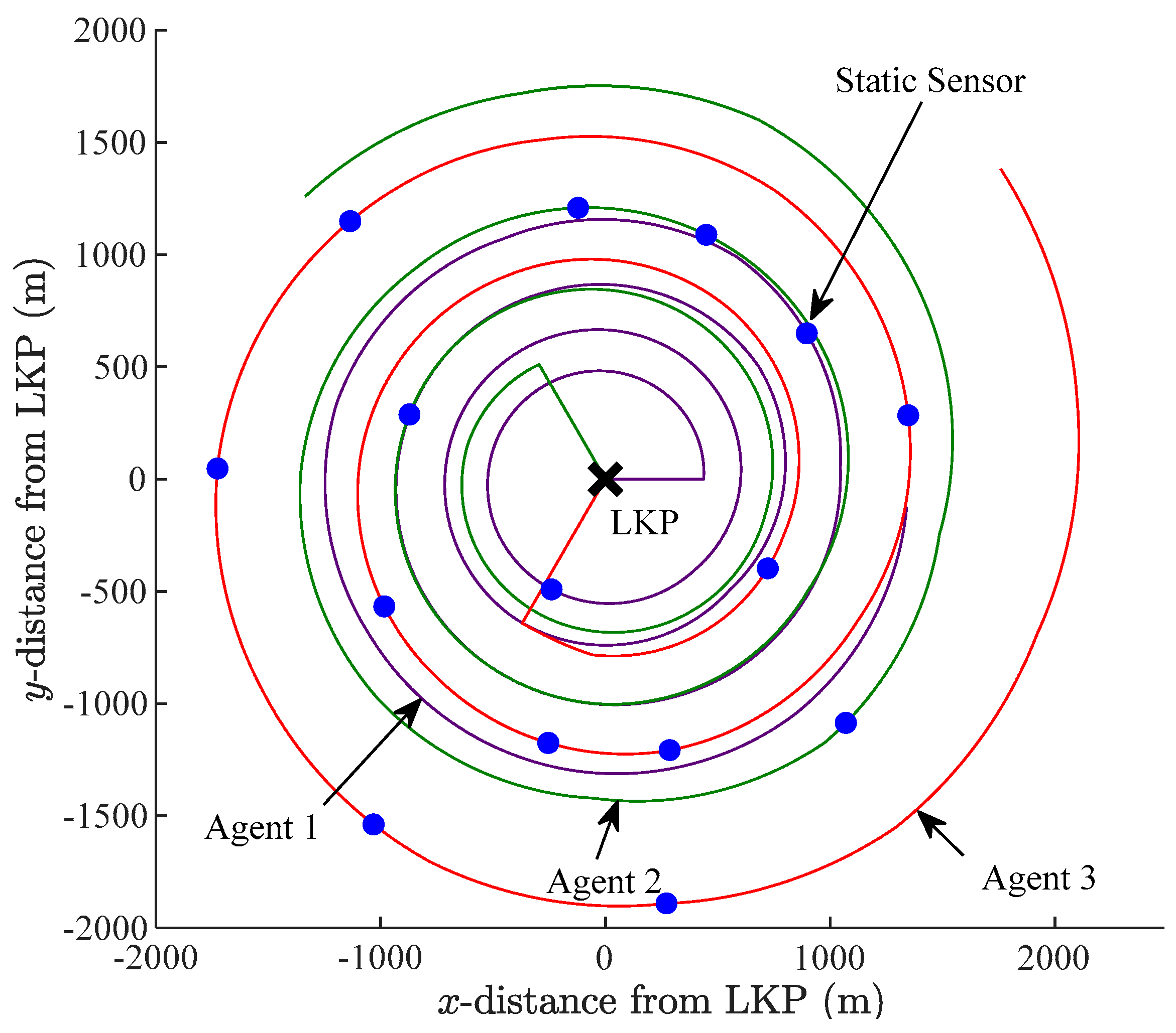
The search trajectories planned are optimal in that they distribute search effort optimally across a set of iso-probability curves. Since the curves themselves are optimally selected to maximize a weighted sum of success rate and search time metrics, the planned mobile-agent search is optimal. One may note that search trajectories can optimally remain on iso-probability curves since these curves, by definition, are continuous closed curves that encircle the LKP and propagate smoothly over time. An example set of agent trajectories for three agents originating from the LKP, assigned to the 25%, 50%, and 75% iso-probability curves, respectively, is illustrated in Figure 3. All trajectories start at the LKP and move outwards.

3.1.2. Sensor-Network Deployment Planning

An optimal sensor-network deployment, herein, is one which maximizes the probability of target detection while remaining adaptive and directionally unbiased. A globally optimal deployment satisfying all these qualities could be planned if sensor deployment positions and times were unconstrained. In this work, however, sensor deployment positions are constrained by the previously planned agent trajectories. The approach taken herein is to minimize the error between the characteristics of the global optimal network and the planned constrained network. The error metric is described in further detail below. The description is then followed by an algorithm for optimizing the sensor network to minimize the metric.

Optimization Metric

Herein, the constrained optimization problem is solved by considering an overall sensor-network deployment error metric, $\Psi \left({\mathit{N}}_s\right)$. This metric comprises three parts: (a) detection probability error, ${\mathrm{e}}_{\mathrm{p}}$, (b) angular positional error, $e_a$, and (c) temporal distribution error, $e_t$:

$$\Psi \left({\mathit{N}}_s\right)=e_p\left({\mathit{N}}_s\right)+e_a\left({\mathit{N}}_s\right)+e_t\left({\mathit{N}}_s\right).$$

(4)

Above, a linear (unweighted) sum of errors is considered as all three types of error are equally important to minimize. Validation of the optimization metric and its correlation with actual sensor network performance is demonstrated at the end of this section. A description of each of these error components is provided below.

(a) Detection probability error $\left({\mathrm{e}}_{\mathrm{p}}\right)$

In order to formulate a metric for detection probability error, time-cumulative likelihood of target detection needs to be defined. The likelihood of a target being at a position $\mathit{X}=\mathit{x}$, at time $\mathit{T}=t$, can be expressed as:

$$\rho \left(\mathit{x},t\right)=P\left(\mathit{X}=\mathit{x}|\mathit{T}=t\right),$$

(5)

where random variables for position and time are represented by $\mathit{X}$ and $\mathit{T}$, respectively. It follows directly that the time-cumulative likelihood of target detection over a time interval $\left[t_a,t_b\right]$ is:

$${\rho }_c\left(\mathit{x},t_a,t_b\right)={{\displaystyle \int }}_{t_a}^{t_b}\rho \left(\mathit{x},t\right)dt.$$

(6)

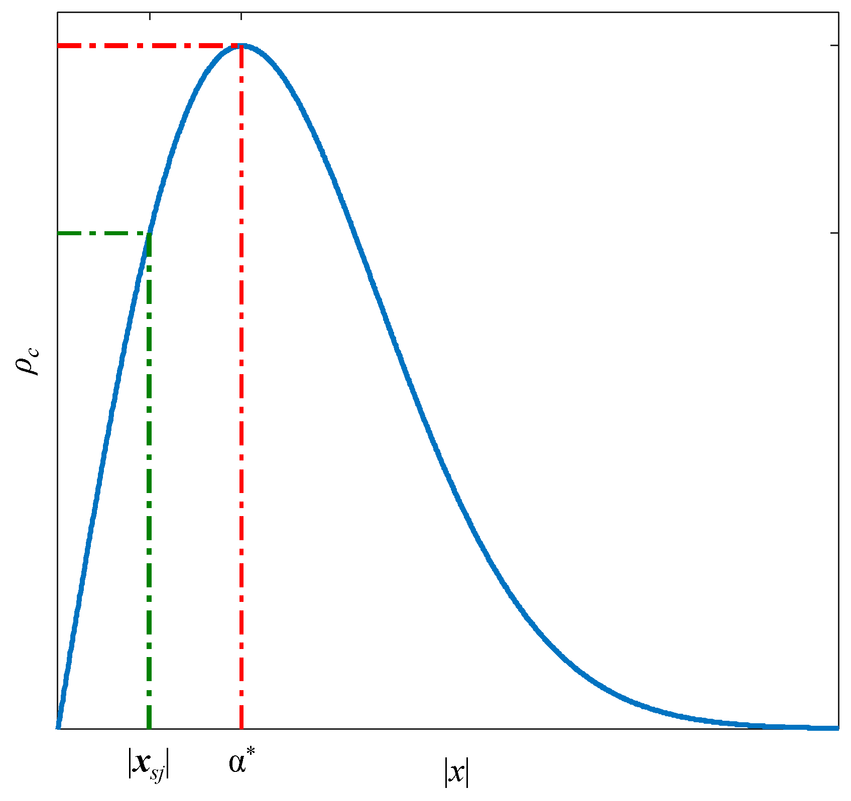
Let us assume that ${\mathit{x}}_{\mathit{s}\mathit{j}}$ represents the actual position at which Sensor $j$ will be deployed at time $t_{sj}$. The direction in which this sensor is deployed, relative to the LKP, is given by ${\theta }_j=\mathrm{atan}\left(y_{sj}/x_{sj}\right)$. The ideal position for the sensor in the same direction, ${\mathit{x}}_{sj}^{*}\left({\theta }_j\right)$ can be expressed as a vector of length ${\alpha }^{*}$ in the direction ${\theta }_j$:

$${\mathit{x}}_{sj}^{*}\left({\theta }_j\right)={\alpha }^{*}{\left[\cos \left({\theta }_j\right),\sin \left({\theta }_j\right)\right]}^{\top },$$

(7)

where ${\alpha }^{*}$ is a constant that maximizes ${\rho }_c$:

$${\alpha }^{*}=\underset{\alpha }{\mathrm{argmax}}{\rho }_c\left(\mathsf{\alpha }{\left[\cos \left({\theta }_j\right),\sin \left({\theta }_j\right)\right]}^{\top },t_{sj},t_{end}\right).$$

(8)

Figure 4 illustrates the position of ${\alpha }^{*}$ along the time-cumulative likelihood of target detection in a given direction.

The ideal deployment of static sensors is one where each sensor is placed at the ideal deployment position at its corresponding deployment time. The time-cumulative probabilistic target detection error, $e_p$, is, therefore, the average percentage difference between the time-cumulative likelihood of detection that could be achieved at the ideal deployment position and the time-cumulative likelihood of detection achieved at the actual deployment position:

$$e_p=\frac{1}{n}{\displaystyle \sum }_{j=1}^n\left|\frac{{\rho }_c\left({\mathit{x}}_{\mathit{s}\mathit{j}}^{*},t_{sj},t_{end}\right)-{\rho }_c\left({\mathit{x}}_{\mathit{s}\mathit{j}},t_{sj},t_{end}\right)}{{\rho }_c\left({\mathit{x}}_{\mathit{s}\mathit{j}}^{*},t_{sj},t_{end}\right)}\right|.$$

(9)

One may note that $e_p$ increases for deployment plans that have sensors deployed at positions with lower time-cumulative probability of target detection than the ideal.

It should be noted that no integral over the binary disk is used in Equation (6), since ${\rho }_c$ is a likelihood and not a probability of detection, and that the likelihood representation is maintained all the way through to Equation (9). This is valid under two assumptions that we make. First, the sensing area of a sensor is much smaller than the length scale of fluctuations in the target location probability distribution function. Under this assumption, the probability of target detection by a sensor can be simply computed as a product of the sensing area and the value of the probability distribution function at the sensor location. Second, all sensors have the same sensing radius. Under this assumption, the probability of target detection is related to the likelihood function by a scalar multiplier. When evaluating the performance of a sensor placement, then, the scalar is cancelled out and can be neglected.

(b) Angular positional error $\left({\mathrm{e}}_{\mathrm{a}}\right)$

It is imperative that search resources be distributed throughout the search area such that they maximize the number of possible target motions that could be intercepted. Namely, sensor deployment locations should be diversified to consider a wide variety of possible target motions. Since the direction taken by the target, moving away from the LKP, is unknown, all possible directions of travel should be searched equally. An important objective in the search problem considered, thus, is distributing the sensors in a directionally unbiased manner.

A directionally unbiased search can be planned by distributing the sensors uniformly in an appropriately defined region of interest. This region, in this case, is defined as the area bounded by the set of ideal sensor positions at the first sensor deployment time and the set of ideal sensor positions at the last sensor deployment time. The area can be visualized as one bounded by two closed curves encircling the LKP. The shape of these curves is influenced by a wide variety of factors including the target motion model, the terrain, and obstacles. Obstacles, for example, may cause the space between the two curves to be small. This indicates that the target will cover less ground in the direction of the obstacles due to the obstacles impeding the target’s motion. As a result, fewer sensors would be allocated to the direction in which the obstacles exist.

An equivalent way of expressing the above described ideal distribution is that the number of static sensors deployed in a direction of interest (e.g., an angular region or sector) should be proportional to the range of optimal deployment positions in that direction. Namely, for a given direction, $\theta$, the radial distance between the ideal sensor position at the first sensor deployment time, ${\mathit{x}}_{s1}^{*}\left(\theta \right)$, and the ideal sensor position at the final sensor deployment time, ${\mathit{x}}_{sn}^{*}\left(\theta \right)$, can be used as a measure of how many sensors should be deployed in that direction. Figure 5 illustrates this region of interest.

Then, the normalized cumulative deployment area $\overline{A}\left(\theta \right)$, in the range [0, θ], is defined as:

$$A\left(\theta \right)={{\displaystyle \int }}_0^{\theta }\left({\mathit{x}}_{sn}^{*}\left(\theta ’\right)-{\mathit{x}}_{s1}^{*}\left(\theta ’\right)\right)d\theta ’,$$

(10)

$$\overline{A}\left(\theta \right)=\frac{A\left(\theta \right)}{A\left(2\pi \right)}.$$

(11)

The normalized empirical cumulative distribution of the angular positions of all sensors in a deployment plan along the angle $\theta$ can, then, be formulated as:

$$\begin{gathered} \overline{N}\left(\theta \right)=\frac{1}{n}{\displaystyle \sum }_{j=1}^{n}u\left(\theta -{\theta }_{sj}\right), \\ \theta \in \left[0,2\pi \right] \end{gathered}$$

(12)

where $u\left(\theta \right)$ is the unit step function and ${\theta }_{sj}$ is the angular position of Sensor $j$.

Angular positional error, $e_a$, can, thus, be expressed as the absolute difference between the empirical and ideal distribution of sensor angular positions:

$$e_a=\frac{1}{2\pi }{{\displaystyle \int }}_0^{2\pi }\left|\overline{A}\left(\theta \right)-\overline{N}\left(\theta \right)\right|d\theta .$$

(13)

From this formulation, one can note that the angular distribution error decreases when the empirical cumulative distribution more closely approximates the ideal cumulative distribution.

(c) Temporal distribution error $\left({\mathrm{e}}_{\mathrm{t}}\right)$

In a dynamic search scenario, such as WiSAR, there is always a possibility of discovering information that leads to a higher-accuracy estimate of the target location while the search is in progress (e.g., a clue regarding where the target passed through). Deploying sensors over an extended time interval allows for the possibility of re-planning the deployment of the remaining undeployed sensors when a clue is found. This allows for a significant increase in the probability of target detection soon after a clue is found. An optimal distribution of deployment times would depend on how frequently and when new information might be discovered. If one were to assume that no new information is expected to be found, sensors could have been deployed earlier in the search to further optimize the probability of target detection. On the other hand, if one were to assume that clues would be found frequently, sensor deployments could be held back for a better understanding of where the target is heading. However, since we do not know the frequency or the number of potential dropped clues, one would be better off to assume that the target is uniformly likely do so at any time during the user defined interval within which sensors are to be deployed. An optimal distribution of deployment times in this case is one in which the deployment of search effort over the interval is temporally unbiased. This can be achieved by deploying sensors throughout the search to achieve a uniform rate of search-effort deployment. Assuming the deployment of Sensor $j$ at a given deployment time, $t_{sj}$, implies deploying a certain amount of search effort, $G\left(t_{sj}\right)$, the cumulative search effort deployed, for $n$ sensors, would be:

$$E\left(t\right)={\displaystyle \sum }_{j=1}^{n}u\left(t-t_{sj}\right)G\left(t_{sj}\right).$$

(14)

An expression for normalized cumulative search effort, $\overline{E}\left(t\right)$, is, then, formulated to be:

$$\overline{E}\left(t\right)=\frac{E\left(t\right)}{E\left(t_{sn}\right)}.$$

(15)

Temporal distribution error, ${\mathrm{e}}_{\mathrm{t}}$, is, then, defined by:

$$e_t=\frac{{{\displaystyle \int }}_{t_{start}}^{t_{last}}\left|\overline{E}\left(t\right)-\left(Mt+B\right)\right|dt}{{{\displaystyle \int }}_{t_{start}}^{t_{last}}\left(Mt+B\right)dt},$$

(16)

where $t_{start}$ is the time the search starts relative to the best estimated time the target left the LKP, and $t_{last}$ is a pre-defined last sensor deployment time. Figure 6 illustrates the metric. The numerator in (16) represents the error between $\overline{E}\left(t\right)$ and the linear function $\left(Mt+B\right)$, that approximates a constant rate of search effort from $t_{start}$ to $t_{last}$. $M$ and $B$ are constants of this linear function. The greater the value of $e_t$, the greater the deviation from deploying a constant rate of search effort, and the more temporally biased the planned sensor network.

Validation of the Optimization Metric

In order to validate that a reliable relationship exists between $\Psi \left({\mathit{N}}_s\right)$ and the deployed sensor-network’s search performance, multiple unconstrained network deployments were randomly generated for empirical analysis. The deployments were generated by randomly selecting angular and radial sensor positions relative to the LKP from a uniform distribution. The upper bound of the radial position in any direction was defined by the maximum distance the target could possibly travel, which is represented by the 100% iso-probability curve. Deployment times were similarly randomly selected from a uniform distribution. In this case, the lower and upper bounds for the uniform distribution were, themselves, sampled from a uniform distribution with a lower and upper bound of a user-defined $t_{start}$ and $t_{last}$. This approach was taken to randomly generate many different variations of temporal bias. For each deployment plan, the network’s deployment error, $\Psi \left({\mathit{N}}_s\right)$, and the network’s search performance were calculated.

Search performance error, ${ϵ}_{perf}$, is defined, herein, as a function of a network’s target detection rate, $\Gamma$, mean detection time, $\tau$, and temporal unbiasedness (measured in terms of the temporal distribution error, $e_t$):

$${ϵ}_{perf}=\left(1-\Gamma \right)+\frac{\tau }{{\tau }_{max}}+e_t,$$

(17)

where the constant ${\tau }_{max}$ is equal to the largest mean detection time by any sensor network considered.

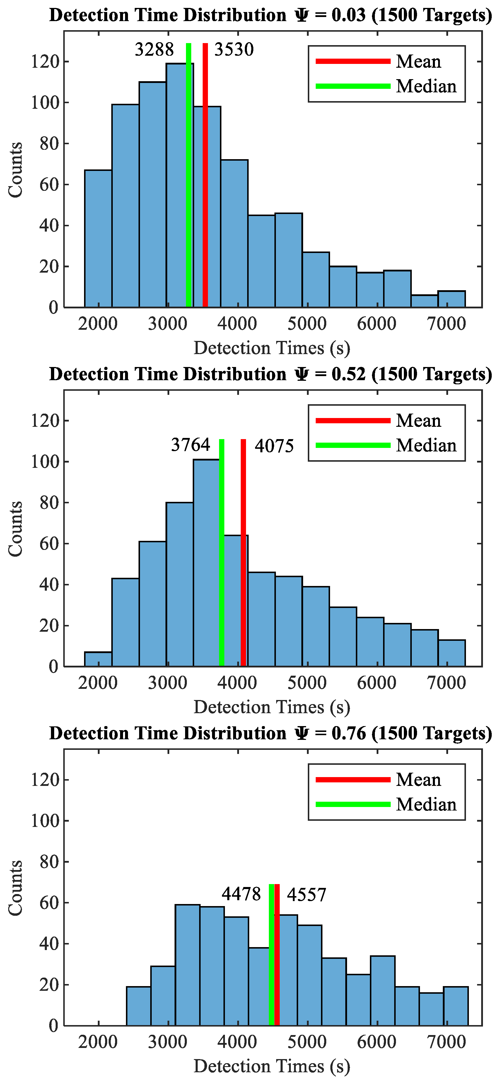
In order to compute the metrics for a given network, numerous simulated searches were run, and the metrics were computed from the results obtained. Each run consisted of a target starting its random motion (specified by the motion model) with a given randomly sampled walking speed at the LKP and recording a search success or failure. If successful, the time at which the target was detected is recorded. The search performance error is, then, calculated to evaluate its overall performance. The detection rate, $\Gamma$, was computed as the proportion of simulated searches that were successful (i.e., the proportion of simulated targets that were detected). The mean detection time was calculated as the mean time at which targets were detected in successful searches. This implies that only the detection times of successful searches contributed to calculating $\tau$. The mean detection time metric is normalized by ${\tau }_{max}$ such that this portion of the performance metric is on the same order of magnitude as the mean detection time and temporal distribution error metrics. Namely, the mean detection time metric (originally in the order of ${10}^2~{10}^4$) is scaled to match the order of the detection rate and adaptability portions of the metric (${10}^0$). One may note that using the median deployment time would have yielded near-identical results. An analysis of the mean and median values showed little difference between the two across multiple sensor deployments. Figure 7 shows the histogram of target detection times for three different sensor networks of varying quality, $\Psi =0.03$, $\Psi =0.52$, and $\Psi =0.76$, demonstrating the minimal difference between the mean and median detection times. Finally, temporal unbiasedness was determined by computing the temporal distribution error defined in Equation (16). A linear, unity-weighted sum is used to combine the three metrics as they are all considered equally important in the context of this work. Variable weights could, naturally, be added to each term in the sum to emphasize the importance of one metric over the others if desired.

A total of 2260 different network deployments were randomly generated to validate the optimization metric. Target detection rate and mean detection time were both evaluated by conducting simulated experiments, with $t_{start}$ = 1800 s, $t_{last}$ = 3600 s, and $t_{end}$ = 7200 s. For each sensor network deployment plan, 1500 different simulated searches were run to evaluate its performance. In each search, target motion was generated using the motion model described in Section 2.1 with ${\sigma }_{\theta }=\mathsf{\pi }/3\mathrm{rad}$ and $d_{max }=100 \mathrm{m}$. The target walking speed for each simulated search was sampled from a normal distribution with a mean of $\mu =0.15\mathrm{m}/\mathrm{s}$ and a standard deviation of $\sigma =0.05\mathrm{m}/\mathrm{s}$. Each deployment plan utilized a total of 76 sensors. The results are illustrated in Figure 8.

In Figure 8, the optimized network constructed by our proposed approach assuming unconstrained sensor deployments is also plotted. One may note that it yielded the lowest $\Psi \left({\mathit{N}}_s\right)$ value (red ×). This is the unconstrained optimal sensor deployment previously mentioned in Section 2.2. Based on these results, it was concluded that a lower $\Psi \left({\mathit{N}}_s\right)$ value indeed corresponds to better search performance for a static-sensor network.

Optimization Algorithm

The minimization of $\Psi \left({\mathit{N}}_s\right)$ directly is intractable for multiple reasons. For example, both the objective function $\Psi \left({\mathit{N}}_s\right)$ and the constraints that the minimization is subject to are non-linear and non-differentiable. The high dimensionality and large solution space of the problem due to its scaling with the number of mobile agents and static sensors considered also contributes to intractability. Trajectory constraints presented in (3) also introduce an additional challenge in that feasible sensor deployment positions in space are directly related to time. Namely, sensor deployment times and positions cannot be sequentially optimized.

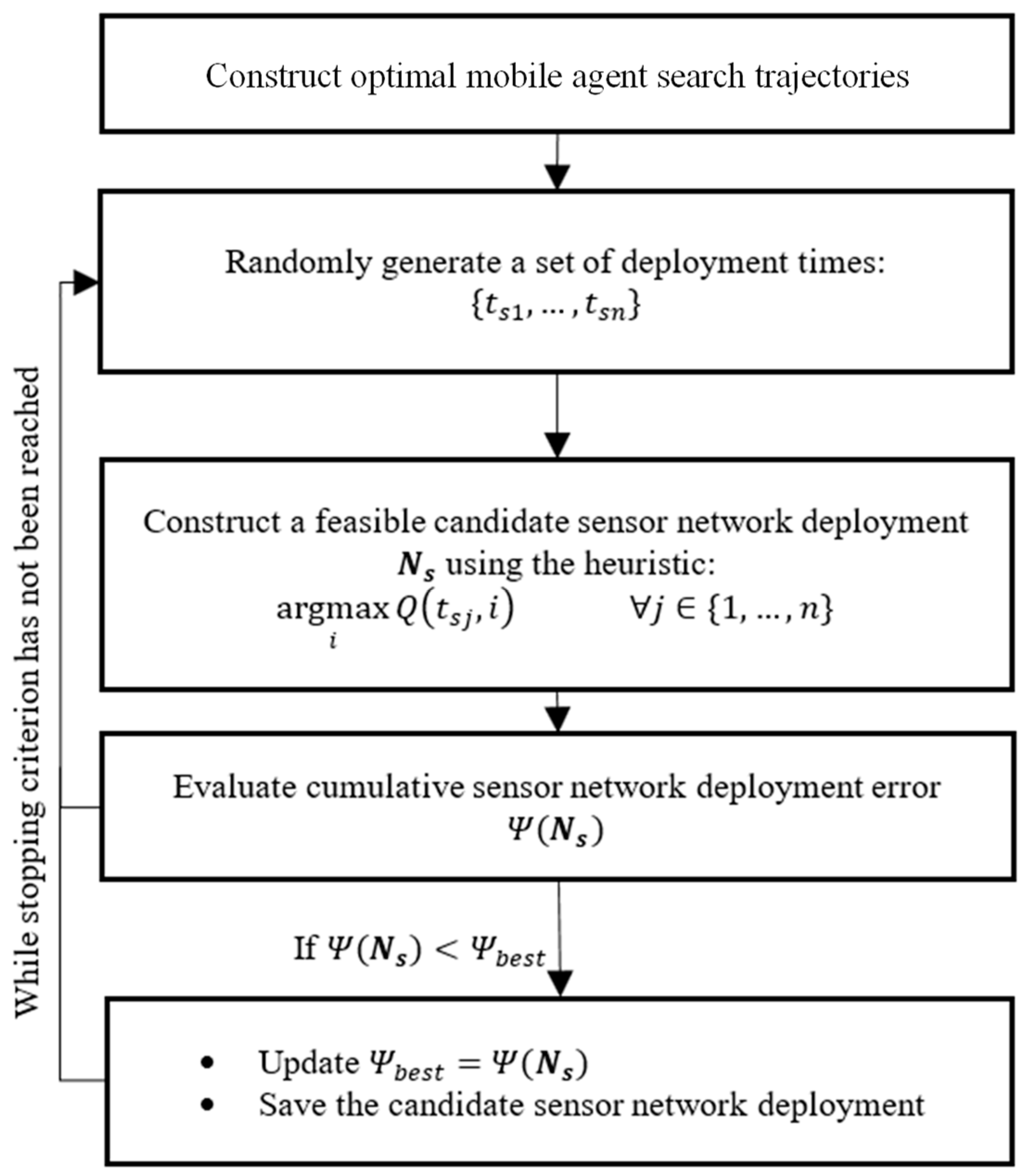
Considering the above complications, an iterative, heuristic-based solution algorithm is proposed herein to determine a near-optimal trajectory-constrained sensor network, Figure 9. This algorithm involves constructing multiple near-optimal solutions from multiple random starts and choosing the best-found solution as the deployment plan to be implemented. One may note that “near-optimal” here refers to a time-limited solution. Namely, it refers to a solution obtained by allowing an optimization algorithm to run until some time limit is reached. It is as close (near) to global optimal as the algorithm could reach within the allotted time. During planning, thus, the proposed optimization algorithm is executed for the entire duration of the limited time available. In the context of this paper (i.e., WiSAR search planning), the optimization algorithm is allowed to run until the search resources arrive in the field and the search needs to begin.

Planning begins with a random selection of deployment times in the range $\left[t_{start},t_{last}\right]$. With deployment times fixed, a heuristic is used to greedily select the agent whose position maximizes the quality of a sensor deployment, $Q$, for each deployment time. The quality of a sensor deployment is computed considering the deployment’s optimality in terms of time-cumulative likelihood of target detection, as well as how spatially distributed the sensor is with respect to the rest of the network. As such, the sensor deployment quality of Sensor $j$ deployed at time $t_{sj}$ by Agent $i$ is defined as:

$$Q\left(t_{sj},i\right)=\varrho \left(t_{sj},i\right)+S\left(t_{sj},i\right).$$

(18)

The first term above, $\varrho \left(t_{sj},i\right)$, represents the likelihood of a sensor deployment detecting the target in this case. Namely, it is the ratio between a Sensor $j$’s time-cumulative likelihood of target detection if it was to be deployed at time $t_{sj}$ at Agent $i$’s position, and the maximum time-cumulative likelihood of target detection achievable if Sensor $j$ was to be deployed at the ideal deployment position in the same direction at time $t_{sj}$:

$$\mathit{\varrho }\left({\mathit{t}}_{\mathit{s}\mathit{j}},\mathit{i}\right)=\frac{{\mathit{\rho }}_{\mathit{c}}\left({\mathit{x}}_{\mathit{r}\mathit{i}},{\mathit{t}}_{\mathit{s}\mathit{j}},{\mathit{t}}_{\mathit{e}\mathit{n}\mathit{d}}\right)}{{\mathit{\rho }}_{\mathit{c}}\left({\mathit{x}}_{\mathit{s}\mathit{j}}^{*},{\mathit{t}}_{\mathit{s}\mathit{j}},{\mathit{t}}_{\mathit{e}\mathit{n}\mathit{d}}\right)}.$$

(19)

The second term in (18), $S\left(t_{sj},i\right)$, is a spatial metric that considers how spread out the next planned sensor deployment will be relative to any previously planned sensor deployments. This results in an overall increase spread of sensors throughout the search area. Maximizing spread diversifies sensor deployment locations and, thus, covers a larger number of possible target motions. This term is the ratio that quantifies how far the considered sensor deployment is from all previously planned sensor deployments:

$$S\left(t_{sj},i\right)=\frac{\min \left|d\left({\mathit{x}}_{sw},{\mathit{x}}_{ri}\left(t_{sj}\right)\right)\right|}{d_{largest}\left(t_{sj}\right)}.$$

(20)

Above, $d\left({\mathit{x}}_{sw},{\mathit{x}}_{ri}\left(t_{sj}\right)\right)$ is the Euclidean distance between the sensor position ${\mathit{x}}_{sw}$ of an already planned sensor deployment $w$, and the position ${\mathit{x}}_{ri}\left(t_{sj}\right)$ of Agent $i$, which is being considered for sensor deployment at time $t_{sj}$. The numerator, then, is the distance between a deployment position under consideration and the nearest already planned sensor deployment. In the denominator, the term $d_{largest}$ takes on the value of the greatest $\min \left|d\left({\mathit{x}}_{sw},{\mathit{x}}_{ri}\left(t_{sj}\right)\right)\right|$ evaluated up to the considered deployment of Sensor $j$.

Therefore, for each deployment time, Agent $i_j^{*}$ that maximizes $Q$ is selected to deploy Sensor $j$:

$$i_j^{*}=\underset{i}{\mathrm{argmax}}Q\left(t_{sj},i\right).$$

(21)

It should be noted that the probabilistic component $\varrho$ and spatial spread component $S$ approximate $e_p$ and $e_a$ respectively in $\Psi \left({\mathit{N}}_s\right)$. Maximizing $\varrho$ will tend to reduce $e_p$, while maximizing $S$ will tend to reduce $e_a$. The difference between maximizing sensor deployment quality $Q,$ and minimizing cumulative sensor network deployment error $\Psi \left({\mathit{N}}_s\right)$, is that $Q$ quantifies the quality of a single sensor deployment at a single deployment time $t_{sj}$, while $\Psi \left({\mathit{N}}_s\right)$ considers the error associated with the complete static-sensor network deployment (i.e., for the entire sensor network). One may also note that the selection of agents is not constrained by a fixed inventory of sensors on each agent at this point. Namely, after the search is planned and prior to starting its search, each agent will be loaded with the exact number of sensors it is planned to deploy.

In order to minimize $\Psi \left({\mathit{N}}_s\right)$, the proposed heuristic algorithm is iterated for as many times as allowable during WiSAR planning, Figure 9. This allows for the evaluation of many possible deployment plans to find a near-optimal solution. This approach is taken as there is often a limited amount of time available to plan a search (i.e., planning with a deadline) and a heuristic approach cannot guarantee a globally optimal sensor network. The generation of a random set of deployment times is proposed at each iteration since it will allow the heuristic to explore a wider range of the solution space. The solution with the smallest value of $\Psi \left({\mathit{N}}_s\right)$ is kept as the best-found sensor deployment plan that should be implemented during execution.

Figure 10 presents a simple example of a sensor network consisting of 15 sensors planned on the same three mobile agent trajectories shown in Figure 3. The algorithm was executed with a stopping criterion of 300 iterations to generate the sensor network shown.

3.2. Re-Planning

The above detailed hybrid search-planning process may need to be re-initiated when new target-motion information becomes available during the search. Information could be discovered, for example, in the form of clues left behind by the target (e.g., clothing, footprints, etc.). These clues can be found by agents as they search the region of interest. Re-planning follows the same process as the initial planning. Namely, optimal agent trajectories are re-planned first, followed by sensor-network deployment re-planning around the new clue position, all starting from the point at which the clue was found. One may note that, while a clue could give some indication of the target’s travel direction since leaving the LKP, it must not be used to bias search planning to favor any direction. The target, since leaving the LKP, could have changed its heading for any number of reasons. The target could have, for example, dropped the clue after it realized it was lost and was heading back to the LKP. The proposed method, thus, continues to consider all possible directions as being equally likely travel directions for the target in search re-planning.

Re-planning of agent trajectories first requires each agent to reach its assigned iso-probability curve in the shortest travel time, $t_{travel}$, possible. As such, agents are re-assigned to re-planned iso-probability curves to minimize (the maximum) overall travel time, so that all agents are re-deployed as soon as possible. This agent-to-curve re-assignment problem can be formulated as a Linear Bottleneck Assignment Problem (LBAP) and solved efficiently in polynomial time using a threshold algorithm given in reference [61], as was done in previous work [4]. After the re-assignment is complete, agent trajectories are planned to first intercept their new iso-probability curves in the shortest amount of time. Then, agent trajectory planning continues with the planning of optimal search trajectories as described in Section 3.1.1. Namely, trajectories are planned for agents to remain on their assigned iso-probability curves as the curves propagate.

Following trajectory re-planning is sensor-network deployment re-planning. Namely, determining when and where the remaining (undeployed) sensors will be placed along the re-planned agent trajectories. The new static-sensor network is planned as described in Section 3.1.2, with the additional constraint that the sensor supply of individual agents is limited. Namely, since agents cannot return to a central location to restock or transfer sensors between them, they have a fixed number of (undeployed) sensors on them when re-planning occurs. As such, a capacity constraint must be placed on each agent such that it will not be planned to deploy more sensors than it has available for deployment. This capacity constraint was not present in initial planning since it was assumed that any number of sensors could be loaded onto any agent.

If a chronological deployment time sequence is always used in the sensor-deployment- planning algorithm, the agents with fewer sensors will be unable to deploy sensors later in the search. In order to alleviate this problem resulting from the capacity constraint, the order of deployment times considered for agent selection is randomized in subsequent iterations of the construction algorithm.

Finally, re-planning differs from initial planning in that additional consideration is given to the set of already deployed sensors. A subset of the sensors that were deployed prior to re-planning are considered when computing $Q.$ Namely, the positions of some already deployed sensors are taken into consideration during sensor-network re-planning since ignoring them may cause redundant coverage of the search area. The sensors that could provide redundant coverage are defined to be those within the region where sensors could be redeployed.

4. Simulated Search Examples

The hybrid search-planning method proposed in this paper was validated via multiple simulated WiSAR search scenarios.

4.1. Example 1: Target Search

In this example, the target’s walking speed of 0.22 m/s was sampled from a normal distribution for the pertinent demographic group according to ($\mu$ = 0.24 m/s, $\sigma$ = 0.08 m/s). The motion model also involved the target wandering up to a maximum degree of ${\sigma }_{\theta }$ = π /3 rad, while maintaining a given heading up to a maximum distance of $d_m$ = 100 m.

A total of ten mobile agents and 135 static sensors were made available for the search. Each static sensor had a sensing range of 10 m, while the agents all had a sensing range of 5 m. The agents were capable of moving at a speed of 2.4 m/s.

Following the notification of the missing target, the search started at $t_{start}$ = 3600 s, with all agents being at the LKP. The last static sensor was deployed at $t_{last}$ = $t_{s135}$ = 10,800 s, with the overall end of search time being $t_{end}$ = 12,600 s.

Figure 11 illustrates the complete initial plan of optimal agent trajectories and the static-sensor network. Figure 12, in turn, shows the end of the search, with the target (green ×) being successfully located by Agent #4 at (−497 m, 1404 m) at time $t$ = 10,140 s. In this figure, the target path traveled is shown by a magenta-colored line, originating from the LKP (black $\times$). The positions of 118 already deployed sensors (blue dots) and current agent positions (black squares) are also indicated.

4.2. Example 2: Target Search with Re-Planning

In this example, the same target motion model, search environment, and search time parameters that were in Example 1 are utilized. The target walking speed was 0.20 m/s for this experiment.

Search resources provided included ten mobile agents and 90 static sensors. Each static sensor had a sensing radius of 20 m, and each agent had a sensing radius of 10 m. All agents were assumed to travel at a constant speed of 2.4 m/s.

Figure 13 presents the complete initial plan of optimal agent trajectories and the static sensor network. Figure 14, in turn, shows a snapshot of the search, where Agent #2 has found a clue that was dropped by the target at (−178 m, −960 m) (cyan ×) at time $t$ = 7503 s. At this point of time, 39 sensors have already been deployed (blue dots).

The discovery of the clue, as shown in Figure 14, triggers re-planning of the search. The resulting re-planned agent trajectories and remaining sensor deployments are shown in Figure 15. Figure 16, in turn, shows the end of the search with the target being successfully located (green ×) at (−333 m, −1280 m) by Sensor #36 at time $t$ = 9577 s. A total of 68 static sensors have been deployed by this time.

5. Comparative Study

The search-planning approach proposed in this paper was compared to the sensor-centric WiSAR search-planning method outlined in reference [62]. In reference [62], the motion trajectories of a team of multiple agents were planned to carry out the scheduled deployment of an optimal static-sensor network while allowing the agents to be on the look-out for the target as they were moving from one deployment position to another. Namely, in this approach, the (global) unconstrained optimal sensor network is planned first. Agent motions are, then, planned with the primary objective of deploying the sensors according to the set optimal schedule.

As will be shown below through extensive experiments, it is hypothesized here that, although in certain search scenarios, the two hybrid approaches would perform comparably, in cases where the sensors could not be deployed at their (global) optimal times and positions, as dictated by reference [62], due to few available agents, the agent-centric approach proposed herein would perform significantly better than the sensor-centric approach detailed in reference [62]. Since it would be difficult to predict ahead of time which approach the user should select in a real WiSAR scenario, our recommendation is that prior to the start of a search for a lost person, both approaches be simulated in parallel and the hybrid plan produced by the method with the greater potential to succeed quickly be chosen for implementation.

5.1. Two Comparative Experiments

As an example of how the proposed agent-centric and alternative sensor-centric approach can be compared, the result of using a search plan generated by the sensor-centric method on the two search examples in Section 4 are presented herein. In Example 1, detailed in Section 4.1, the target was found at (−605 m, 1420 m) at time $t$ = 10,798 s by Agent #5. This outcome, as expected, although slightly worse, is comparable to the one obtained through the method described in this paper, i.e., $t$ = 10,140 s.

Similarly, Example 2 detailed in Section 4.2. was also addressed using the sensor-centric method. In this case, the target was found at (−462 m, −1400 m) at time $t$ = 10,641 s by Sensor #82. This outcome, as expected, although worse, is still comparable to the one obtained through the method described in this paper, i.e., $t$ = 9577 s.

5.2. Large Sets of Simulations

In order to compare the proposed agent-centric method with the alternative sensor-centric method, numerous simulated searches were run for each search scenario and performance metrics were computed from the results obtained. Namely, in the experiments examined in this sub-section, 1000 different target motions were simulated for each scenario and the number of targets found (out of 1000) by the search planned by each method was examined for making a comparison. Targets were assumed to be found if they passed within the sensing radius of a sensor or an agent. The primary focus of these experiments was to investigate the impact of various agent-to-sensor combinations on the search success of our method versus the one proposed in [62]. The search success rate for a given search scenario was selected as the metric of scrutiny because it most accurately represents the true concern at hand (i.e., the probability of finding the target, in a real-life mobile-target search scenario).

In the search scenarios simulated, demographics information was used to infer normally-distributed target walking speeds ($\mu$ = 0.24 m/s, $\sigma$ = 0.08 m/s). A target motion model, previously described in Section 2.1, with angular heading deviations of ${\sigma }_{\theta }$ = π/3 rad, and $d_m$ = 100 m, was assumed. Target-motion simulation, then, consisted generating a path and simulating the target following this path using a walking speed sampled from the aforementioned target walking speed distribution.

Each search began at $t_{start}$ = 3600 s after the target was known to be at the LKP and was planned to continue until $t_{end}$ = 53,000 s, with the latest static sensor deployment at $t_{last}$ = 10,800 s. A search was considered successful if the target was found by a static sensor or a mobile agent before $t_{end}$.

Table 1. Target-detection Comparison—1000 Trials.

# of Agents	# of Sensors	# of Targets Found by Proposed Method	# of Targets Found by Method in [62]	Improvement over [62] (%)	Significance Confidence (%)
10	45	352	325	8	63.3
2	45	183	125	46	98.9
2	90	278	128	117	99.9

shows the results of the experiments where the static sensors had a sensing radius of 15 m and the mobile agents had a sensing radius of 3 m.

As can be noted from Table 1, in cases where the sensors could not be deployed at their (global) optimal times and positions, as dictated by [62], due to few available agents, the proposed agent-centric method performed significantly better (with 98.9% and 99.9% confidence by confidence interval analysis) than the sensor-centric approach–last two rows of the table. Namely, a large gap in detection rate performance is attributable to multiple extremely late sensor deployments, as determined by reference [62]. Moreover, a “snowball effect” was observed where one late sensor deployment led to further and increasingly other late sensor deployments. Unlike the method proposed in reference [62], the approach presented in this paper is robust to low agent-sensor ratios due to the trajectory-constraints sensor deployments are subject to. It should be noted that both hybrid methods performed significantly better when static sensors were present than when they were not. Namely, both methods found 216 and 46 targets, with 10 and 2 agents, respectively. One may note that the hybrid methods performed identically when no static-sensors are present as they both reduce to the method presented in references [4,20,21].

6. Conclusions

This paper proposes a novel hybrid-search planning strategy where autonomous mobile search agents are supported by a static-sensor network. The agent trajectories are planned first, to maximize the likelihood of target detection. The planning of static-sensor deployments, constrained to the already planned agent trajectories, then follows.

The strategy is novel in that the mobile agents deploy static sensors without deviating from their optimal search trajectories. The trajectory-constrained sensor network is planned to maximize the likelihood of target detection, while maintaining temporal and directional unbiasedness in target motion over the course of the search. The proposed planning method utilizes an objective function quantifying the error between the considered and ideal static sensor-network deployment plan to optimize sensor deployments. A strong correlation was established between this error metric and actual sensor-network search performance. Planning of the sensor network was done via an iterative heuristic-based algorithmic approach with randomly initialized deployment times to efficiently minimize the error metric. The proposed method was validated via simulated WiSAR experiments.

Simulations were also used to compare the search performance with the proposed hybrid search method and that of a sensor-centric hybrid planning approach (where sensor deployment planning occurs prior to mobile agent trajectory planning). Results of the simulations showed that the proposed hybrid method outperforms the sensor-centric method in reference [62] when the optimal sensor network is not realizable. As such, it is suggested that the proposed agent-centric and the sensor-centric method be run in parallel and their results evaluated through simulation when choosing a search plan in an actual WiSAR scenario.

The search strategy presented in this work is not limited to WiSAR and can be applied to any general mobile-target search problem, assuming target-motion model and target-location likelihood information are provided or can be estimated. While this paper proposes an iterative heuristic algorithmic model to minimize sensor network deployment error, future work could include an investigation of more efficient optimization methods that yield trajectory-constrained sensor networks with better search performance.

References

- Berger, J.; Lo, N. An innovative multi-agent search-and-rescue path planning approach. Comput. Oper. Res. 2015, 53, 24–31. [Google Scholar] [CrossRef]
- Doherty, P.J.; Guo, Q.; Doke, J.; Ferguson, D. An analysis of probability of area techniques for missing persons in Yosemite National Park. Appl. Geogr. 2014, 47, 99–110. [Google Scholar] [CrossRef]
- Israel, M.; Khmelnitsky, E.; Kagan, E. Search for a mobile target by ground vehicle on a topographic terrain. In Proceedings of the IEEE Convention of Electrical & Electronics Engineers in Israel, Eilat, Israel, 14–17 November 2012; pp. 1–5. [Google Scholar]
- Macwan, A.; Nejat, G.; Benhabib, B. Optimal Deployment of Robotic Teams for Autonomous Wilderness Search and Rescue. In Proceedings of the IEEE/RSJ International Workshop on Intelligent Robots and Systems, San Francisco, CA, USA, 25–30 September 2011; pp. 4544–4549. [Google Scholar]
- Wong, E.-M.; Bourgault, F.; Furukawa, T. Multi-vehicle Bayesian Search for Multiple Lost Targets. In Proceedings of the IEEE Robotics and Automation Society’s, Barcelona, Spain, 18–22 April 2005; pp. 3169–3174. [Google Scholar]
- Champagne, L.; Carl, E.G.; Hill, R. Search theory, agent-based simulation, and u-boats in the Bay of Biscay. In Proceedings of the Simulation Conference, New Orleans, LA, USA, 7–10 December 2003; pp. 991–998. [Google Scholar]
- Arora, A.; Dutta, P.; Bapat, S.; Kulathumani, V.; Zhang, H.; Naik, V.; Mittal, V.; Cao, H.; Demirbas, M.; Gouda, M.; et al. A line in the sand: A wireless sensor network for target detection, classification, and tracking. Comput. Netw. 2004, 46, 605–634. [Google Scholar] [CrossRef]
- Kehagias, A.; Mitsche, D.; Prałat, P. Cops and invisible robbers: The cost of drunkenness. Theor. Comput. Sci. 2013, 481, 100–120. [Google Scholar] [CrossRef]
- Lin, L.; Goodrich, M.A. Hierarchical heuristic search using a gaussian mixture model for UAV coverage planning. IEEE Trans. Cybern. 2014, 44, 2532–2544. [Google Scholar] [CrossRef] [PubMed]
- Zhao, W.; Meng, Q.; Chung, P.W.H. A Heuristic distributed task allocation method for multivehicle multitask problems and its application to search and rescue scenario. IEEE Trans. Cybern. 2016, 46, 902–915. [Google Scholar] [CrossRef] [PubMed]
- Keller, C.M. Applying optimal search theory to inland SAR: Steve Fossett case study. In Proceedings of the Conference on Information Fusion, Edinburgh, UK, 26–29 July 2010; pp. 1–8. [Google Scholar]
- Hohzaki, R. A cooperative game in search theory. Nav. Res. Logist. NRL 2009, 56, 264–278. [Google Scholar] [CrossRef]
- Benkoski, S.J.; Monticino, M.G.; Weisinger, J.R. A survey of the search theory literature. Nav. Res. Logist. NRL 1991, 38, 469–494. [Google Scholar] [CrossRef]
- Grundel, D.A. Searching for a moving target: optimal path planning. In Proceedings of the IEEE Netw. Sens. Control, Tucson, AZ, USA, 19–22 March 2005; pp. 867–872. [Google Scholar]
- Goodrich, M.A.; Morse, B.S.; Engh, C.; Cooper, J.L.; Adams, J.A. Towards using Unmanned Aerial Vehicles (UAVs) in Wilderness Search and Rescue: Lessons from field trials. Interact. Stud. 2009, 10, 453–478. [Google Scholar]
- Ding, Y.F.; Pan, Q. Path planning for mobile robot search and rescue based on improved ant colony optimization algorithm. Appl. Mech. Mater. 2011, 66–68, 1039–1044. [Google Scholar] [CrossRef]
- Xiao, H.; Cui, R.; Xu, D. A sampling-based bayesian approach for cooperative multiagent online search with resource constraints. IEEE Trans. Cybern. 2017, 48, 1773–1785. [Google Scholar] [CrossRef] [PubMed]
- Pack, D.J.; DeLima, P.; Toussaint, G.J.; York, G. Cooperative control of UAVs for localization of intermittently emitting mobile targets. IEEE Trans. Syst. Man Cybern. Part B Cybern. 2009, 39, 959–970. [Google Scholar] [CrossRef] [PubMed]
- Agcayazi, M.T.; Cawi, E.; Jurgenson, A.; Ghassemi, P.; Cook, G. ResQuad: Toward a semi-autonomous wilderness search and rescue unmanned aerial system. In Proceedings of the International Conference Unmanned Aircraft Syst., Arlington, VA, USA, 7–10 June 2016; pp. 898–904. [Google Scholar]
- Macwan, A.; Vilela, J.; Nejat, G.; Benhabib, B. Multi-robot deployment for wilderness search and rescue. Int. J. Robot. Autom. 2016, 31, 10.2316/Journal.206.2016.1.206–4366. [Google Scholar] [CrossRef]
- Macwan, A.; Vilela, J.; Nejat, G.; Benhabib, B. A multirobot path-planning strategy for autonomous wilderness search and rescue. IEEE Trans. Cybern. 2015, 45, 1784–1797. [Google Scholar] [CrossRef] [PubMed]
- Rogge, J.A.; Aeyels, D. Multi-robot coverage to locate fixed and moving targets. In Proceedings of the Control Application Intelligence Control, St. Petersburg, Russia, 8–10 July 2009; pp. 902–907. [Google Scholar]
- Lavis, B.; Furukawa, T.; Durrant Whyte, H.F. Dynamic space reconfiguration for Bayesian search and tracking with moving targets. Auton. Robots 2008, 24, 387–399. [Google Scholar] [CrossRef]
- Sung, Y.; Furukawa, T. Information measure for the optimal control of target searching via the grid-based method. In Proceedings of the International Conference on Information Fusion, Heidelberg, Germany, 5–8 July 2016; pp. 2075–2080. [Google Scholar]
- Yuan, H.; Xiao, C.; Zhan, W.; Wang, Y.; Shi, C.; Ye, H.; Jiang, K.; Ye, Z.; Zhou, C.; Wen, Y.; et al. Target detection, positioning and tracking using new UAV gas sensor systems: Simulation and analysis. J. Intell. Robot. Syst. 2018, 1–12. [Google Scholar] [CrossRef]
- Hanna, D.; Ferworn, A.; Lukaczyn, M.; Abhari, A.; Lum, J. Using Unmanned Aerial Vehicles (UAVs) in locating wandering patients with dementia. In Proceedings of the IEEE/ION Position, Location and Navigation Symposium, Monterey, CA, USA, 23–26 April 2018; pp. 809–815. [Google Scholar]
- Amaldi, E.; Capone, A.; Cesana, M.; Filippini, I. Design of wireless sensor networks for mobile target detection. IEEEACM Trans. Netw. 2012, 20, 784–797. [Google Scholar] [CrossRef]
- Clouqueur, T.; Phipatanasuphorn, V.; Ramanathan, P.; Saluja, K.K. Sensor deployment strategy for detection of targets traversing a region. Mob. Netw. Appl. 2003, 8, 453–461. [Google Scholar] [CrossRef]
- Phipatanasuphorn, V.; Ramanathan, P. Vulnerability of sensor networks to unauthorized traversal and monitoring. IEEE Trans. Comput. 2004, 53, 364–369. [Google Scholar] [CrossRef]
- Lazos, L.; Poovendran, R.; Ritcey, J.A. Detection of mobile targets on the plane and in space using heterogeneous sensor networks. Wirel. Netw. 2009, 15, 667–690. [Google Scholar] [CrossRef]
- Yoon, Y.; Kim, Y.-H. An Efficient Genetic Algorithm for maximum coverage deployment in wireless sensor networks. IEEE Trans. Cybern. 2013, 43, 1473–1483. [Google Scholar] [CrossRef]
- Mukherjee, K.; Gupta, S.; Ray, A.; Wettergren, T.A. Statistical-mechanics-inspired optimization of sensor field configuration for detection of mobile targets. IEEE Trans. Syst. Man Cybern. Part B Cybern. 2011, 41, 783–791. [Google Scholar] [CrossRef]
- Karatas, M.; Craparo, E.; Akman, G. Bistatic sonobuoy deployment strategies for detecting stationary and mobile underwater targets. Nav. Res. Logist. NRL 0 2018, 65, 331–346. [Google Scholar] [CrossRef]
- Vilela, J.; Kashino, Z.; Ly, R.; Nejat, G.; Benhabib, B. A dynamic approach to sensor network deployment for mobile-target detection in unstructured, expanding search areas. IEEE Sens. J. 2016, 16, 4405–4417. [Google Scholar] [CrossRef]
- Kashino, Z.; Kim, J.Y.; Nejat, G.; Benhabib, B. Spatiotemporal adaptive optimization of a static-sensor network via a non-parametric estimation of target location likelihood. IEEE Sens. J. 2017, 17, 1479–1492. [Google Scholar] [CrossRef]
- Shue, S.; Conrad, J.M. A survey of robotic applications in wireless sensor networks. In Proceedings of the IEEE Southeastcon, Jacksonville, FL, USA, 4–7 April 2013; pp. 1–5. [Google Scholar]
- Lambrou, T.P.; Panayiotou, C.G.; Felici, S.; Beferull, B. Exploiting Mobility for Efficient Coverage in Sparse Wireless Sensor Networks. Wirel. Pers. Commun. 2009, 54, 187–201. [Google Scholar] [CrossRef]
- Suzuki, T.; Sugizaki, R.; Kawabata, K.; Hada, Y.; Tobe, Y. Autonomous deployment and restoration of sensor network using mobile robots. Int. J. Adv. Robot. Syst. 2010, 7, 105–114. [Google Scholar] [CrossRef]
- Li, X.; Fletcher, G.; Nayak, A.; Stojmenovic, I. Randomized carrier-based sensor relocation in wireless sensor and robot networks. Ad Hoc Netw. 2013, 11, 1951–1962. [Google Scholar] [CrossRef]
- Li, X.; Falcon, R.; Nayak, A.; Stojmenovic, I. Servicing wireless sensor networks by mobile robots. IEEE Commun. Mag. 2012, 50, 147–154. [Google Scholar] [CrossRef]
- Wang, Y.; Wu, C.H. Robot-assisted sensor network deployment and data collection. In Proceedings of the International Symposium on Computational Intelligence in Robotics and Automation, Jacksonville, FI, USA, 20–23 June 2007; pp. 467–472. [Google Scholar]
- Deshpande, N.; Grant, E.; Henderson, T.C. Target localization and autonomous navigation using wireless sensor networks—A pseudogradient algorithm approach. IEEE Syst. J. 2014, 8, 93–103. [Google Scholar] [CrossRef]
- Woiceshyn, K.; Kashino, Z.; Nejat, G.; Benhabib, B. Vehicle routing for resource management in time-phased deployment of sensor networks. IEEE Trans. Autom. Sci. Eng. 2018, 16, 716–728. [Google Scholar] [CrossRef]
- Mateo, D.; Horsevad, N.; Hassani, V.; Chamanbaz, M.; Bouffanais, R. Optimal network topology for responsive collective behavior. Sci. Adv. 2019, 5, eaau0999. [Google Scholar] [CrossRef] [Green Version]
- Wagner, T.; Lesser, V. Evolving real-time local agent control for large-scale multi-agent systems. In Intelligent Agents VIII, Proceedings of the International Workshop on Agent Theories, Architectures, and Languages, Seattle, WA, USA, 1–3 August 2001; Meyer, J.-J.C., Tambe, M., Eds.; Springer: Berlin, Heidelberg, Germany, 2002; pp. 51–68. [Google Scholar] [CrossRef]
- Long, M.; Su, H.; Liu, B. Group controllability of two-time-scale multi-agent networks. J. Frankl. Inst. 2018, 355, 6045–6061. [Google Scholar] [CrossRef]
- Lin, L.; Goodrich, M.A. A bayesian approach to modeling lost person behaviors based on terrain features in wilderness search and rescue. Comput. Math. Organ. Theory 2010, 16, 300–323. [Google Scholar] [CrossRef]
- Hayat, S.; Yanmaz, E.; Brown, T.X.; Bettstetter, C. Multi-objective UAV path planning for search and rescue. In Proceedings of the IEEE International Conference on Robotics and Automation, Singapore, 29 May–3 June 2017; pp. 5569–5574. [Google Scholar]
- Niedzielski, T.; Jurecka, M.; Miziński, B.; Remisz, J.; Ślopek, J.; Spallek, W.; Witek-Kasprzak, M.; Kasprzak, Ł.; Świerczyńska-Chlaściak, M. A real-time field experiment on search and rescue operations assisted by unmanned aerial vehicles. J. Field Robot. 2018, 35, 906–920. [Google Scholar] [CrossRef]
- Liu, Y.; Nejat, G. Multirobot cooperative learning for semiautonomous control in urban search and rescue applications. J. Field Robot. 2016, 33, 512–536. [Google Scholar] [CrossRef]
- Ramirez-Paredes, J.P.; Doucette, E.A.; Curtis, J.W.; Gans, N.R. Urban target search and tracking using a UAV and unattended ground sensors. In Proceedings of the American Control Conference, Chicago, IL, USA, 1–3 July 2015; pp. 2401–2407. [Google Scholar]
- Yu, H.; Meier, K.; Argyle, M.; Beard, R.W. Cooperative path planning for target tracking in urban environments using unmanned air and ground vehicles. IEEEASME Trans. Mechatron. 2015, 20, 541–552. [Google Scholar] [CrossRef]
- Zhang, Z.; Nejat, G.; Guo, H.; Huang, P. A novel 3D sensory system for robot-assisted mapping of cluttered urban search and rescue environments. Intell. Serv. Robot. 2011, 4, 119–134. [Google Scholar] [CrossRef]
- Hong, A.; Igharoro, O.; Liu, Y.; Niroui, F.; Nejat, G.; Benhabib, B. Investigating human-robot teams for learning-based semi-autonomous control in urban search and rescue environments. J. Intell. Robot. Syst. 2019, 94, 669–686. [Google Scholar] [CrossRef]
- Chung, T.H.; Hollinger, G.A.; Isler, V. Search and pursuit-evasion in mobile robotics. Auton. Robots 2011, 31, 299–316. [Google Scholar] [CrossRef] [Green Version]
- Zheng, J.; Yu, H.; Liang, W.; Zeng, P. Probabilistic strategies to coordinate multiple robotic pursuers in pursuit-evasion games. In Proceedings of the IEEE International Conference on Robotics and Biomimetics, Sanya, China, 15–18 December 2007; pp. 559–564. [Google Scholar]
- Körner, F.; Speck, R.; Göktogan, A.H.; Sukkarieh, S. Autonomous airborne wildlife tracking using radio signal strength. In Proceedings of the IEEE/RSJ International Workshop on Intelligent Robots and Systems, Taipei, Taiwan, 18–22 October 2010; pp. 107–112. [Google Scholar]
- Bakhtari, A.; Naish, M.D.; Eskandari, M.; Croft, E.A.; Benhabib, B. Active-vision-based multisensor surveillance—An implementation. IEEE Trans. Syst. Man Cybern. Part C Appl. Rev. 2006, 36, 668–680. [Google Scholar] [CrossRef]
- Koester, R.J. Lost Person Behavior: A Search and Rescue Guide on Where to Look for Land, Air and Water; dbS Productions: Charlottesville, VA, USA, 2008. [Google Scholar]
- Croft, E.A.; Benhabib, B.; Fenton, R.G. Near-time optimal robot motion planning for on-line applications. J. Robot. Syst. 1995, 12, 553–567. [Google Scholar] [CrossRef]
- Burkard, R.M.; Dell’Amico, S. Martello Assignment Problems; SIAM, Society for Industrial and Applied Mathematics: Philadelphia, PA, USA, 2009. [Google Scholar]
- Kashino, Z.; Nejat, G.; Benhabib, B. A hybrid strategy for target search using static and mobile sensors. IEEE Trans. Cybern. 2018, 1–13. [Google Scholar] [CrossRef]
Figure 1.
A conceptual illustration of the problem addressed in this paper.
Figure 2.
Iso-probability curves at (a) some time, , and (b) sometime later, .
Figure 3.
Search trajectories for three mobile agents assigned to the 25% (purple), 50% (green), and 75% (red) iso-probability curves.
Figure 4.
The position of and along a time-cumulative likelihood of target detection function in a given direction.
Figure 5.
The region of interest when considering angular positional error.
Figure 6.
The temporal error (blue) is the area between the empirical cumulative effort deployed (red) and the ideal, linear cumulative effort function (black).
Figure 7.
Target detection time histograms with mean and median indicated for several different networks of varying quality.
Figure 8.
A correlation between static sensor network deployment error and search performance error for various static sensor networks.
Figure 9.
Proposed iterative algorithm for the construction of an effective agent-centric hybrid search-plan.
Figure 10.
Planned sensor network.
Figure 11.
Initial plan of agent trajectories and static sensor network for Example 1.
Figure 12.
End of search for scenario in Example 1.
Figure 13.
Initial plan of agent trajectories and static sensor network for Example 2.
Figure 14.
Discovery of a clue in Experiment 2.
Figure 15.
Planned and re-planned agent trajectories and sensor deployments for Example 2.
Figure 16.
End of search scenario in Example 2.
© 2019 by the authors. Licensee MDPI, Basel, Switzerland. This article is an open access article distributed under the terms and conditions of the Creative Commons Attribution (CC BY) license (http://creativecommons.org/licenses/by/4.0/).
Share and Cite
MDPI and ACS Style
Chong Lee Shin, J.; Kashino, Z.; Nejat, G.; Benhabib, B. A Sensor-Network-Supported Mobile-Agent-Search Strategy for Wilderness Rescue. Robotics 2019, 8, 61. https://doi.org/10.3390/robotics8030061
AMA Style
Chong Lee Shin J, Kashino Z, Nejat G, Benhabib B. A Sensor-Network-Supported Mobile-Agent-Search Strategy for Wilderness Rescue. Robotics. 2019; 8(3):61. https://doi.org/10.3390/robotics8030061
Chicago/Turabian StyleChong Lee Shin, Jason, Zendai Kashino, Goldie Nejat, and Beno Benhabib. 2019. "A Sensor-Network-Supported Mobile-Agent-Search Strategy for Wilderness Rescue" Robotics 8, no. 3: 61. https://doi.org/10.3390/robotics8030061
Note that from the first issue of 2016, this journal uses article numbers instead of page numbers. See further details here.