Locomotion of a Cylindrical Rolling Robot with a Shape Changing Outer Surface


1
Department of Mechanical Engineering, Kettering University, Flint, MI 48504, USA
2
Department of Mechanical and Aerospace Engineering, Oklahoma State University, Stillwater, OK 74078, USA
3
Amazon Corporation, Sumner, WA 98390, USA
*
Author to whom correspondence should be addressed.
Robotics 2018, 7(3), 52; https://doi.org/10.3390/robotics7030052
Submission received: 27 July 2018
/
Revised: 28 August 2018
/
Accepted: 30 August 2018
/
Published: 10 September 2018
(This article belongs to the Special Issue Mechanism Design for Robotics)
Abstract
:A cylindrical rolling robot is developed that generates roll torque by changing the shape of its flexible, elliptical outer surface whenever one of four elliptical axes rotates past an inclination called trigger angle. The robot is equipped with a sensing/control system by which it measures angular position and angular velocity, and computes error with respect to a desired step angular velocity profile. When shape change is triggered, the newly assumed shape of the outer surface is determined according to the computed error. A series of trial rolls is conducted using various trigger angles, and energy consumed by the actuation motor per unit roll distance is measured. Results show that, for each of three desired velocity profiles investigated, there exists a range of trigger angles that results in relatively low energy consumption per unit roll distance, and when the robot operates within this optimal trigger angle range, it undergoes minimal actuation burdening and inadvertent braking, both of which are inherent to the mechanics of rolling robots that use shape change to generate roll torque. A mathematical model of motion is developed and applied in a simulation program that can be used to predict and further understand behavior of the robot.
1. Introduction
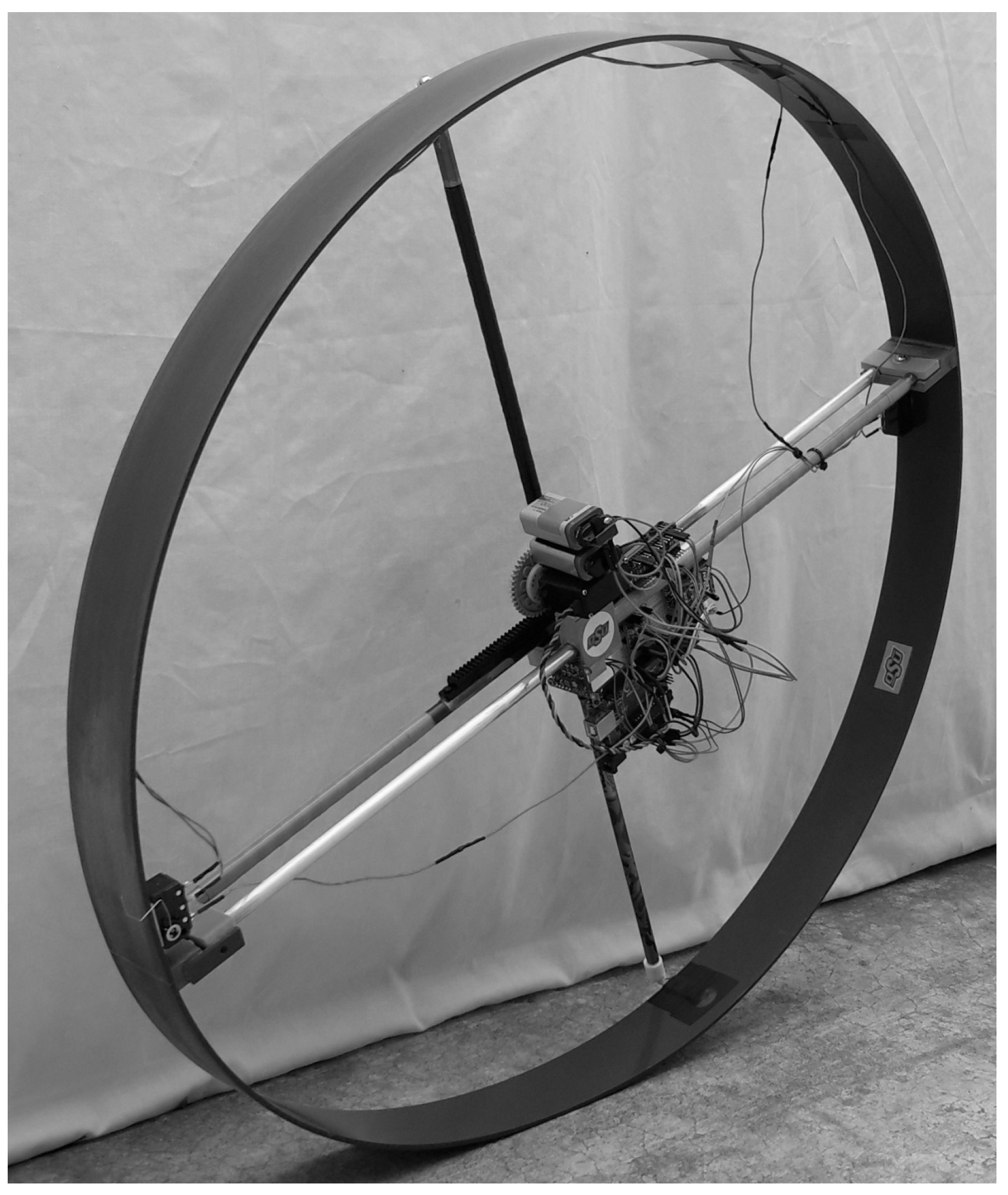
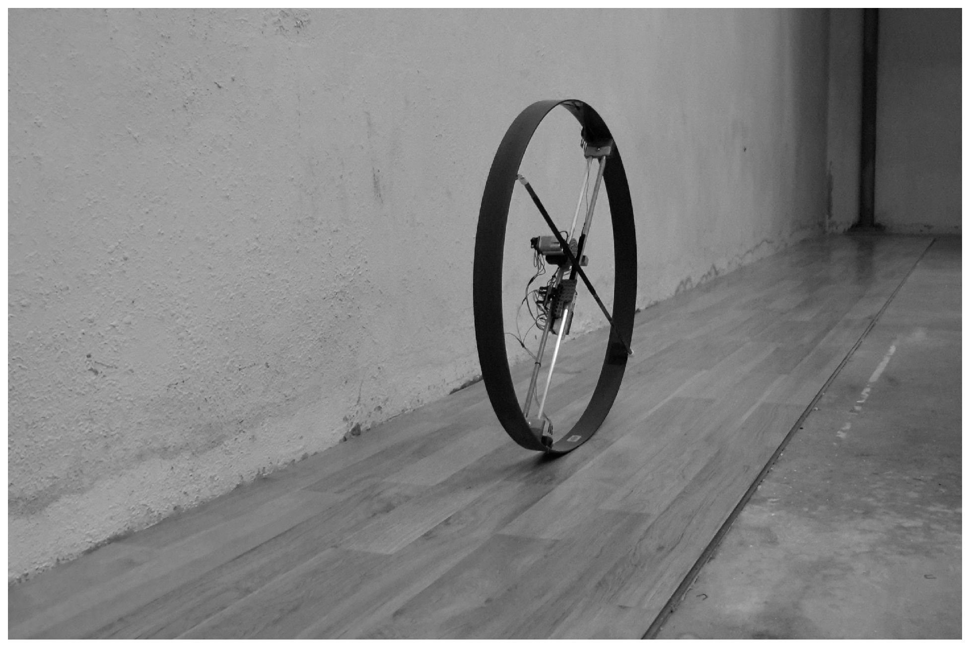
Ground based robots typically move from place to place using wheels, legs, or by changing shape in a biomimetic fashion, as with peristaltic or slithering locomotion [1,2,3]. Wheeled robots are the most common of these three locomotion styles because, in general, wheeled robots are highly efficient and they can move faster than other types of ground based robots [1]. A special class of wheeled robots is the rolling robot, which rolls exclusively on an outer, driven surface that entirely envelopes the system [4]. The study herein investigates locomotion of an autonomous rolling robot, developed at the Unmanned Systems Laboratory at Oklahoma State University (OSU) and pictured in Figure 1, which generates torque by means of changing its outer surface. By executing shape change at just the right time, the robot repeatedly configures itself into a forward-tilting elliptical cylinder and subsequently rolls forward under the force of its own weight. In addition to being shape changing and partially gravity powered, locomotion of the OSU Roller, as it is entitled, is categorized as dynamic [5], meaning it has a natural rocking tendency and exhibits inertial motion. In other words, if the outer surface were to suddenly stop changing shape in the middle of a roll, the robot would likely require several seconds to come to rest. Non-dynamic rollers, such as crawling rolling robots [6,7], move slowly in comparison and do not exhibit dramatic inertial effects after motion input has ceased. The OSU Roller is also an underactuated system [8], referring to how the robot exploits its own natural dynamics in order to achieve steady, rolling locomotion.
Locomotion via gravity power has previously been studied as a field of interest in biomechanics. In [9], researchers presented a mathematical model of human gait using a notional three-link machine with muscles that acted only to periodically configure the gait, leaving the machine to move entirely under the force of gravity for most of its motion. Others [10,11] investigated gaits in which gravity alone generated motion of simple link-composed machines down a slanted ramp. Authors of these studies pointed to the simplicity and efficiency of gravity powered gaits and suggested that power and control could be added using small, strategically timed energy inputs that do not interrupt the natural motion of the machine. Although the OSU Roller is not a linked walking machine like those presented in [10,11], the concept of applying strategically timed inputs during a gravity-powered gait is, in essence, how the OSU Roller works.
With the rise in popularity of modular robotics, researchers have developed shape changing rollers whereby six or more servo motor modules [2] are stacked end-to-end to form a dynamic rolling loop. In [5], researchers presented a modular loop robot composed of ten CKBot modules. On each module of the robot, there was a touch sensor for knowing when a side of the loop was in contact with the ground, at which point the loop quickly morphed into a newly configured football-like shape, now with its long axis aligned closer to the vertical, and continued rolling forward until the next side of the loop touched down. In [12], researchers constructed a modular rolling loop composed of six SuperBot modules that was programmed to deform its shape by contracting and relaxing its hexagonal shape, thereby shifting the robot center of gravity forward and causing the robot to roll. Using their hexagonal rolling loop, researchers performed an experiment that measured endurance by lapping the robot around an inside building corridor for a total distance of roughly one kilometer while voltage in the module batteries was monitored.
Modular loops, while they are highly configurable and allow roboticists to experiment with different locomotion strategies and gaits, are bulky and mechanically complicated systems [13,14]. In contrast to modular loops, researchers in [15] presented a dynamic rolling robot whose outer surface was a thin, lightweight strip of plastic that morphed by means of a singular servo motor. The robot used all onboard sensing and power to achieve velocity control relative to a desired step profile. Results of the research showed that when the robot was given a set of advantageous initial conditions, it was able to accelerate from rest and maintain constant average velocity with significant accuracy. The robot used for the investigation herein, the OSU Roller, is a modified version of the robot presented in [15].
Although shape change has been shown to be a viable locomotion format in the aforementioned research endeavors, the subtle aspects associated with locomotion of dynamic rolling loops have previously not been unearthed. One of these aspects is how driving torque is affected by variation of shape change input timing. Along these lines, a unique characteristic of the OSU Roller is that it has the capability to measure energy consumed by its singular actuator during a trial roll, and this capability is utilized in an experiment documented herein that determines the effect of shape change actuation timing on energy consumption of the robot. Results of this experiment provide insights that can be applied to control shape changing rolling robots, including modular loop robots, more efficiently.
2. Materials and Methods
2.1. Physical Composition of the Robot
The outer surface of the rolling robot is a flat strip of polyvinyl chloride plastic put into the shape of an open, elliptical cylinder. The outer surface is firm enough to provide a steady dynamic roll surface, yet it is limber enough to be reshaped by the pull of a linear actuator positioned along the diameter of the cylinder [15]. When the actuator is not being commanded to move, its static holding force maintains a constant cylindrical shape of the outer surface. On a smooth and level floor, the robot rolls straight without leaning to the side or tipping over, and where the robot meets the floor, the outer surface bends slightly under the weight and motion of the robot. There is negligible slipping of the outer surface against the floor, as verified through high-speed video analysis. The outer surface strip measures cm by cm and has a perimeter of m (Figure 1). Total mass of the robot is kg.
Contained onboard the robot and inside the cylindrical outer surface are a microprocessor board, an inertial measurement unit (IMU) board equipped with a micro-electrical-mechanical gyroscope, two rechargeable 9 V lithium batteries that power the robot, mechanical switches that allow for continual measurement/computation of angular position of the robot, a linear actuator, and an electrical energy sensor. There is also a radio transmitter that sends data regarding robot locomotion to a receiver-equipped, external laptop computer for analysis. The microprocessor is given values of angular position and angular velocity as feedback, and brings about shape change of the outer surface via the linear actuator in order to affect velocity. These hardware components are fastened to the robot in such a way that, even as the actuator elongates and the robot changes shape, the robot center of mass remains approximately in the same location—at the central axis of the outer surface cylinder. A telescoping column orientated in a perpendicular fashion relative to the linear actuator is comprised of male and female tubes whose ends are secured to the inside of the outer surface. This telescoping column, seen in Figure 1, is not a powered actuator. Rather, it serves as an air displacement damper to limit vibration and bending of the outer surface.
In addition to the IMU board and the mechanical switches, a sensor that computes servo motor energy consumption is employed onboard the OSU Roller. At the heart of the sensor is a highly accurate current sensing chip that works in cooperation with a low ohmage resistor placed in series between the motor power supply (a regulated 5 V output from the microprocessor) and the motor load. The sensing chip receives voltage across the resistor, and in turn outputs a voltage that is representative of current that flows into the motor. The representative voltage is received at an analog-to-digital converter on a dedicated microprocessor that is separate from the main microprocessor. In a similar manner, voltage at the positive lead of the servo motor is passed to a second analog-to-digital converter on the dedicated microprocessor. During operation of the robot, a computer program running on the dedicated microprocessor samples these voltages, converts them into values of current, multiplies them for power [16], and then multiplies power by the program’s sample period (200 s) to give energy consumed by the servo motor in the span of one sample period. A running sum gives total electrical energy used by the servo motor since initiation of the program. Every tenth of a second after the computer program has begun, total electrical energy is computed, and these values are passed to the main microprocessor after a trial roll is completed.
2.2. Mathematical Model of Robot Motion
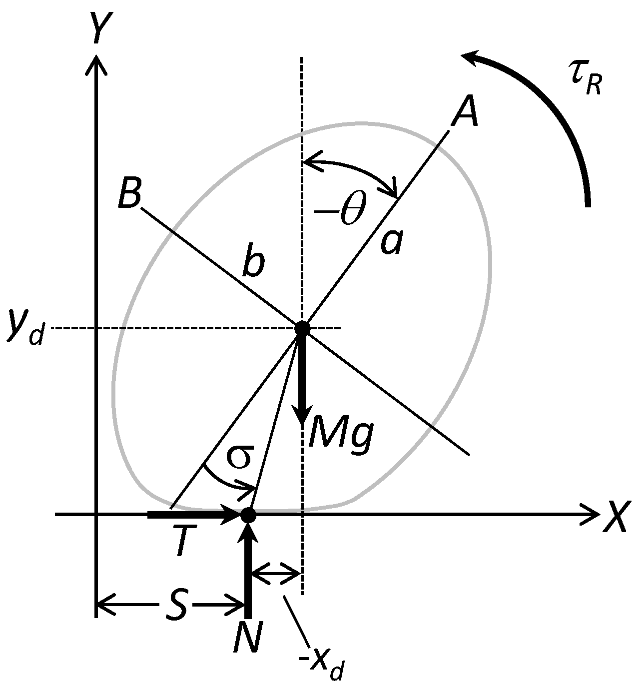
A two-dimensional model of the OSU Roller is developed in which the outer surface is an ellipse with a deflected center due to bending, as illustrated in the free body diagram in Figure 2. The ellipse rolls in one direction along a straight line in the laboratory-fixed Cartesian coordinate frame, , with X as the floor line. A moving rectangular coordinate frame, , is concentrically attached to the ellipse center and rolls with the ellipse. Axis A is coincidental with the actuator line of motion. Lengths a and b of the elliptical semi-major axes are measured along A and B, respectively. The point where the outer surface ellipse touches the floor is denominated as the touch point. The value, , is the horizontal position of the touch point on X with respect to the ellipse center, and is the vertical distance from X to the ellipse center. The angle defined by the positive branch of A and the vertical line passing through is the roll angle of the robot, . (In keeping with the right-hand rule mnemonic [17], is negative with clockwise rotation.) As shown in Figure 2, touch angle, , is defined as the angle made by the A axis and the line from the ellipse center to the touch point:
Touch point location, S, is equivalent to the elliptical arc length integrated over roll angle, plus a constant value [18]:
with
and
Referring to the free body diagram in Figure 2, traction, T, and the normal force, N, act on the robot at the touch point. Weight, , acts at the robot center of mass, which is located at the ellipse center. Rolling resistance torque, , opposes roll motion of the robot. Newton’s second law is applied in the horizontal and vertical directions and also about the center of mass, resulting in three coupled differential equations of motion:
where kg is total mass of the robot. is the time derivative of the angular momentum of the robot about its center of mass, derived by modeling the robot as a collection of point masses that represent the outer surface and hardware components [15]. Equations (5)–(7) are combined into one equation of motion:
where and are constant coefficients of and , respectively, of the term [15,19]. Variables and in Equation (8) are expressed as:
where (, ) is location of the robot center of mass if the outer surface were a perfect ellipse, and and d are changes to and brought on by bending of the outer surface at the floor line, as illustrated in Figure 2. By observing that X is equivalent to the tangent line of the ellipse at the touchpoint, the following expressions are derived for and [13]:
In order to quantify and d, static deflection of the robot center is measured for various orientations of the robot, and the following functions are fitted in relation to an angular position parameter, :
Rolling resistance torque of the outer surface is modeled as , where is a positive value that changes with . This model rightly predicts that when and when . In addition, because d and are never negative during trial rolls, the model rightly predicts that always acts in the clockwise direction, resisting rotation of the robot whenever it moves and bends. The power of two on angular velocity causes the model to capture sharp decelerations that are observed only when the robot moves with relatively high angular velocity. In order to determine appropriate values of , three trial rolls of the robot are performed at three different steady state angular velocities. In the first of these rolls, the robot is controlled to reach rad/s and continue, on average, at this velocity for eight seconds. While the roll is in progress, angular velocity of the rolling robot is sampled using the onboard gyroscope and recorded as a function of time. Afterwards, the simulation program (described subsequently in this section) is run using the same initial conditions as the trial roll. Values of are iteratively used in the program until the simulated response best matches that of the actual robot. Matching is done by comparing total distance rolled and plots of angular velocity at steady state. The value of used in the best match simulation is taken as the appropriate model value: N/s. This process is repeated for rad/s, and the appropriate value of is found to be N/s. For rad/s, the appropriate value of is found to be N/s.
2.3. Robot Velocity Control System
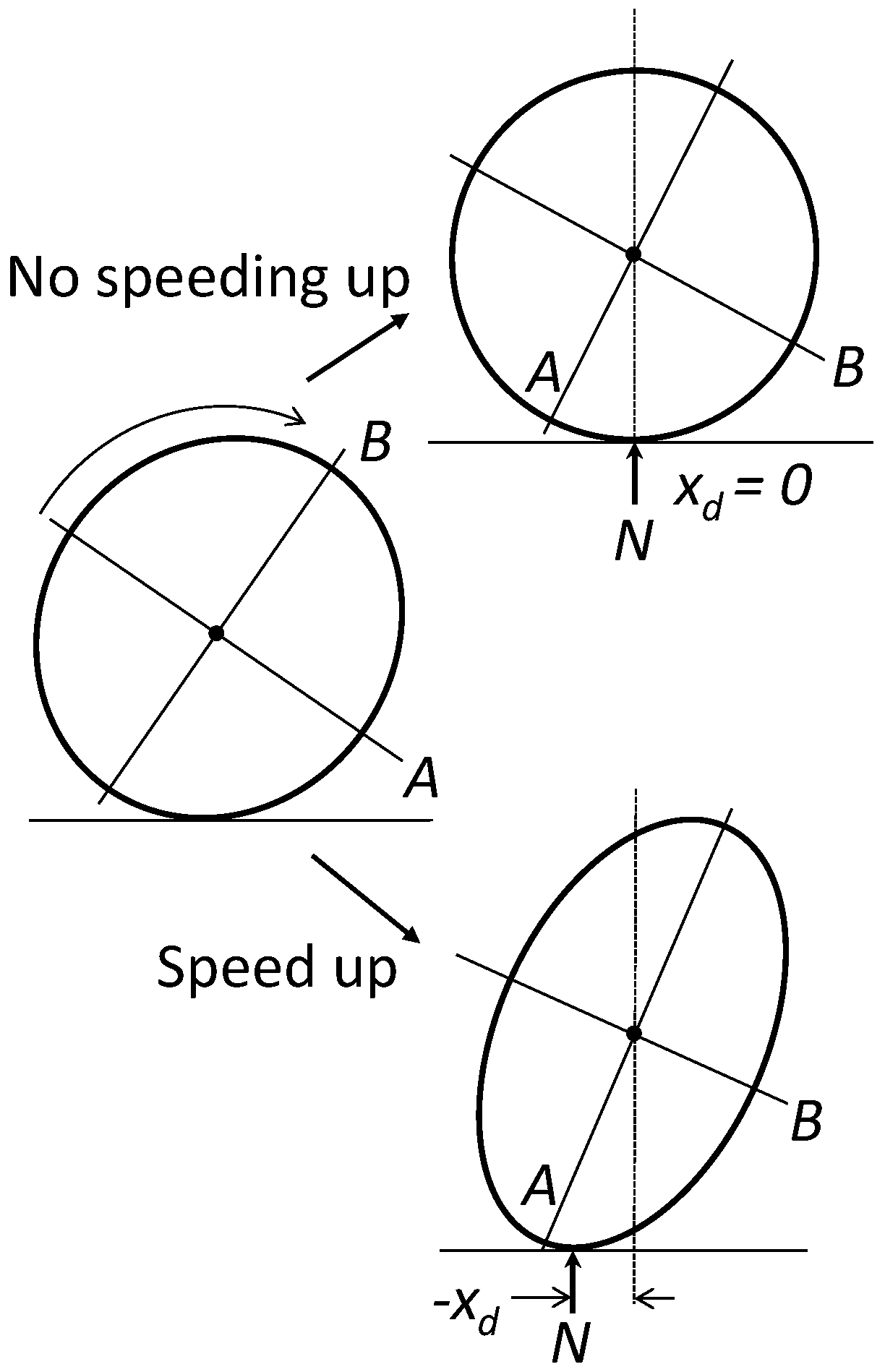
Shape change actuation is triggered when axis A or axis B leans into the roll and passes a certain inclination. When this triggering happens, the robot control system immediately causes the linear actuator to either extend or contract, and the shape of the robot is changed [15]. Upon completion of shape change, the linear actuator remains at the newly changed length until actuation is again triggered. Consider the illustration in Figure 3, in which the rolling robot is shown rolling to the right when shape change actuation is triggered by axis B. The control system responds by changing linear actuator length along axis A, and, consequently, outer surface eccentricity changes as the robot continues to roll to the right. Roughly a quarter-turn after actuation commences, two scenarios are shown in Figure 3. If a has been made longer as A leans into the roll, the robot undergoes an induced torque imbalance about its center of mass that pushes the robot forward and increases speed, as illustrated by the lower ellipse in Figure 3. On the other hand, if a is changed so that the ellipse is now a circle, there is no resulting torque imbalance due to offset, and average speed is not increased.
Shape change actuation is triggered using the concept of tilt. Tilt angle of the robot is
and can be thought of as forward inclination of the robot measured either by A or B relative to the vertical. Tilt angle is used by the control system to perform two actions. First, a special measurement of robot angular velocity () is performed by the onboard gyroscope when newly becomes greater than or equal to a set angle, , which is usually 35° for the trial rolls conducted in the experiment documented herein in Section 2.5.2. This special measurement of angular velocity is referred to as . The second action is actuation triggering, which occurs when newly becomes greater than or equal to the set trigger angle, . In general, as desired speed of the robot increases, must be decreased, or else there is not enough time for the robot to change shape before the next trigger moment. For the experiment documented herein in Section 2.5.2, varies from 25° to 65°.
Upon actuation triggering, the microprocessor prepares for shape change by performing several computations to determine target length of the linear actuator. The first of these computations is that of error:
where is the desired angular velocity, and is a positive constant that is slightly greater than unity. Scaling the desired velocity by is necessary because even when the robot is rolling with nearly the desired velocity (that is, when ), the robot must speed up to compensate for the natural slowing of rolling resistance in order to stay close to the desired angular velocity by the next trigger moment. With computed in this manner, it is in turn used to compute an intermediary value of the target length for the semi-major axis that will be next to lean into the roll [15]. That length is given by
where is equal to m, the radius of the outer surface while in the circular configuration, and is a positive control constant. If is negative (the robot is rolling to the right too slowly), the control system prepares to elongate the semi-major axis relative to the circular configuration. If is positive (the robot is rolling to the right too quickly), is temporarily set to zero until the next trigger moment. In this latter case, the robot assumes the circular configuration and is slowed by rolling resistance. Final target length of the axis is computed according to a saturation operation that ensures the ellipse stays within the physical bounds of the system [15]:
where and are the smallest and largest allowable values of the outer surface semi-major axis due to rotation limits of the actuator servo motor, and they are equal to m and m. Since the linear actuator lies along A, if A is the next axis to lean into the roll, the control system causes the linear actuator to elongate or shorten so that a is equal to . If B is the next axis to lean into the roll, the control system changes a so that b becomes equal to . Time duration of the actuation depends on the orientation of the linear actuator and the magnitude of shape change; when the robot rolls with steady state velocity, time duration of actuation is roughly one-third of a second.
2.4. Simulation Program
A Matlab/Simulink computer program (version R2017a, MathWorks, Natick, MA, USA) is developed to solve Equation (8) numerically for as a function of roll time. The program code is a loop structure that uses initial conditions for and a to solve the equation for at the first pass of the loop. After this first pass, the program “loops back” values that are needed in order to compute . As part of this process, the program checks at each pass to determine if actuation has been triggered, and if it has, a, b, and are newly computed; and are modeled as trapezoidal velocity profiles that, when integrated, give a and b as functions of roll time. Updated values of a, b, , , , and are then looped back, along with values for and obtained through numerical integration, which the program performs using Simulink’s Runge–Kutta [20] solver, and is newly computed. Due to difficulty in finding exact expressions for some of the derivatives on the right side of Equation (8), a numerical derivative algorithm is employed to find the following values: , , , , and . Once is newly computed, it is integrated yet again, and the process is repeated until the simulated roll is completed. At each pass of the loop, motion parameters of the robot, including , are logged and can be plotted as a function of roll time after the program has terminated.
2.5. Experimental Procedure
2.5.1. Control Program
The robot moves under control of a program that is run onboard the microprocessor. The control program is written in C++ programming language, and is essentially an invocation of one primary function [21] named loop that repeats every 10 ms. Prior to loop, the control program has two precursor sections of code that each run only once when the program is executed. The first is a variable definition section, where several variables are set by the user to form a combination of control values and initial conditions that define the trial roll. The variables that can be set are: , , , , and . After the variable definition section, the program performs various initialization tasks, including enablement of microprocessor ports, sensors, communication lines, and moving the actuator to the set value of . After these precursor sections have run, the loop function is finally invoked, but before loop is executed for the first time, the control program sends the energy sensor a digital high voltage signal, causing the sensor to begin the process of measuring current and voltage into the servo motor to compute energy consumed. Roll time of a trial roll begins when this signal is sent, and an LED on the microprocessor board is illuminated as indication. When roll time goes beyond 15 s, the control program electronically detaches the servo motor and enters an idle state until it is manually turned off when the robot is retrieved.
As described in a previous section, position switches are placed on the outer surface of the robot in a manner such that voltage in the switch circuit goes low when one of the position switches is activated, and activation occurs whenever A is in the vertical position, i.e., , , , etc. In the loop function, the control program checks the digital line connected to the switch circuit to see if voltage has gone low since the last cycle of loop. If it has, a flag is momentarily turned on in the program, and a count is tallied of how many times the flag has been turned on since the trial roll began. If loop sees the flag presently on, roll angle of the robot is computed from the flag count. If loop sees the flag presently off, is computed in the sensor program by numerically integrating the sampled angular velocity, according to the trapezoidal rule [20], starting from the last angle measured by the switch circuit.
With computed at every cycle of loop, the control program uses to compute and checks for initiation of angular velocity measurement and an actuation trigger. If angular velocity measurement has been initiated, the current reading of the gyroscope is saved as . If actuation has been triggered, the control program computes and , and then initiates shape change actuation of the robot. Regardless of triggering, at every cycle of loop, the control program computes the predicted values of a, b, and their time-derivatives. Roll distance, S, is also computed at every cycle of loop using an implementation of Equation (2).
The rolling robot possesses a radio transmitter, by which the microprocessor communicates with a receiver-equipped laptop computer located near the roll track. Every 100 ms (or every tenth cycle of loop), the control program transmits several locomotion-related parameters to the laptop, where the parameters are printed as a line of comma separated values to a serial monitor window. The transmitted/printed parameters are: , (which is the same as ), S, a and total energy. In addition, just before entering an idle state, the control program reads the total energy array from the energy sensor and transmits energy values to the laptop computer for every 100 ms of roll time.
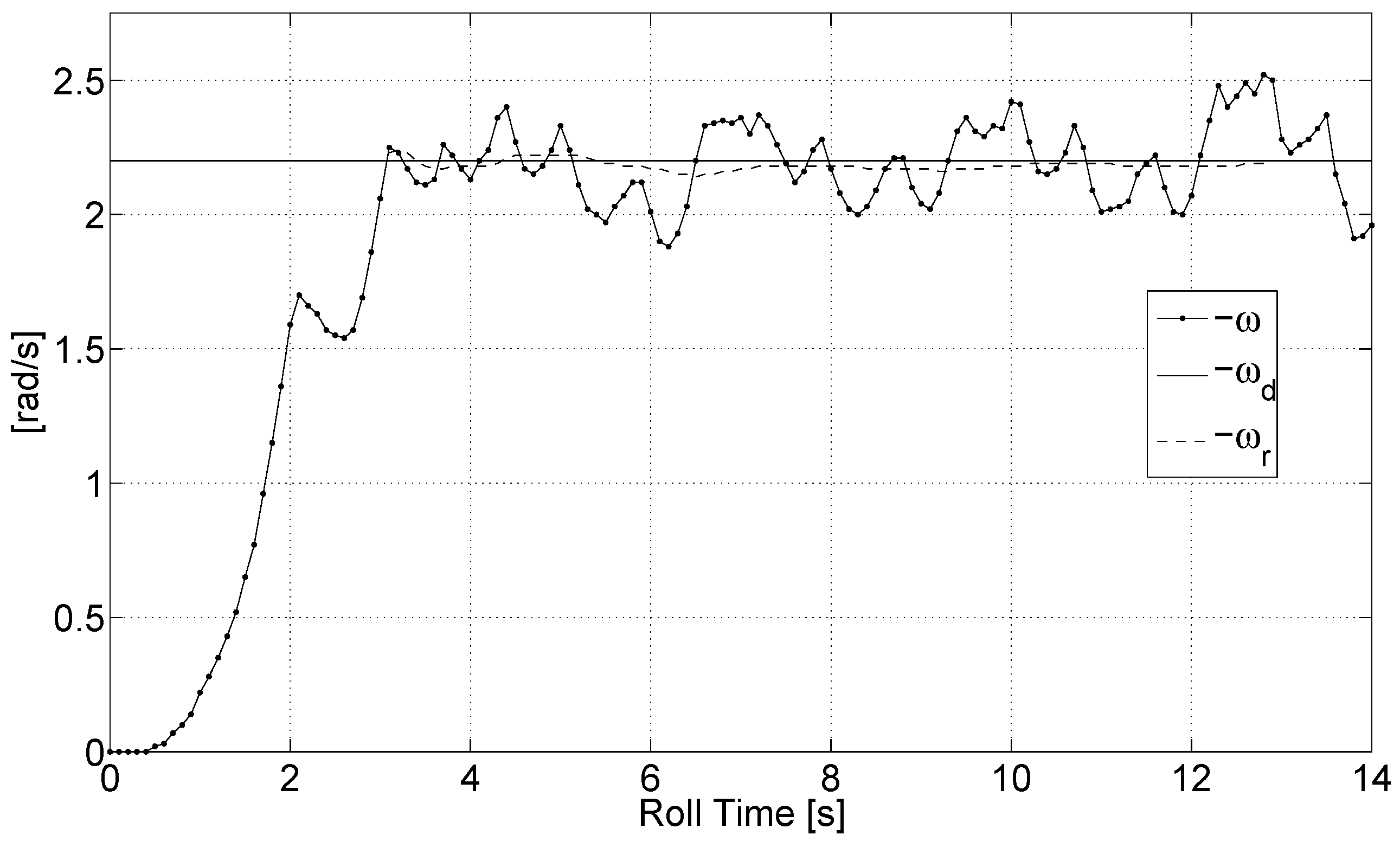
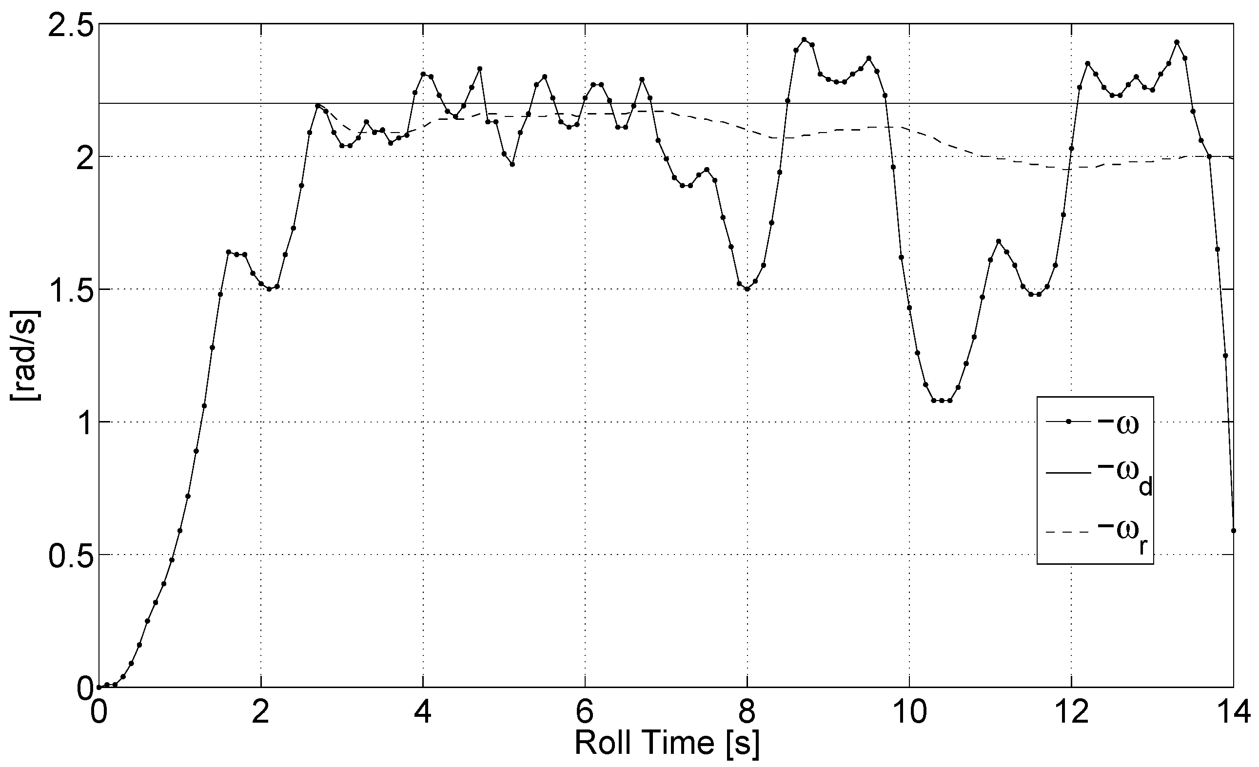
In Figure 4 and Figure 5, angular velocity during two example trial rolls of the robot are plotted versus roll time. In Figure 4, the robot displays stable locomotion, and, in Figure 5, the robot displays unstable locomotion. Stability, as used herein, refers to two conditions being met relative to controlled angular velocity of the robot. The first condition is the robot must speed-up quickly from rest, so that rise time is no more than 6 s. If rise time is longer than 6 s, there is not enough length on the roll track to facilitate a sufficient span of steady state motion for analysis. The second condition is that after robot velocity has risen to , a running average, , of its measured angular velocity must thereafter remain close to the desired constant velocity. Some reasonable variation of within several degrees per second is permissible, but large and fluctuating dips in angular velocity or a steady increase of over time are considered unstable response characteristics.
2.5.2. Trial Rolls
Experimental trial rolls are conducted and provide information used to solve the following three optimization problems:
Find that minimizes for
- rad/s with
- rad/s with
- rad/s with
where is energy consumed per unit roll distance of the robot servo motor, and it is calculated according to a method described in Section 2.5.3. Values of that are suitable for stable locomotion for the various angular velocities have been identified before the experiment is conducted in order to quantify the constraints on for Problems 1–3. Combinations of , and that result in minimization of for the various velocities have also been identified previously and are used in the trial rolls conducted for Problems 1–3.
The experiment starts by fully charging the batteries and allowing the servo motor to remain unpowered for at least three hours to reach the ambient temperature of the laboratory. Next, columns of the linear actuator are cleaned and lubricated, and various parameters in the control program are set. For Problem 1, the desired velocity, , is set to rad/s, is set to 35°, and is set to 35°. Ten preliminary trial rolls of the robot are then conducted in order to warm-up the servo motor. All trial rolls in the experiment are conducted on the same roll track (Figure 6) with a consistent set of initial conditions: , , and m.
A random number generator is employed to shuffle the order of the trial rolls for Problem 1 relative to viable values of . Shuffling is done to avoid any would-be biasing caused by rising temperature of the servo motor. Then, using the order of from the shuffled sequence, 40 trial rolls are conducted in order to collect information to address Problem 1. The first of these trial rolls is conducted with set to the first entry in the sequence, and information from the trial roll is saved. Afterward, is set to the second entry in the sequence, and a second trial roll is conducted, timed to start 45 s after the first roll ends, and information from the trial roll is saved. By the time the last value in the sequence is used, ten trial rolls are conducted for each value of . After trial rolls for Problem 1 are finished, columns of the linear actuator are newly cleaned/lubricated, the batteries are fully recharged, and the motor is allowed to cool. The roll sequence is reshuffled, and is changed to rad/s in order to address Problem 2. For Problem 3, is changed to rad/s. For all problems, the value of is set to 25° when ; otherwise, it is set to 35°.
Upon completing trial rolls for Problems 1–3, saved roll parameters are used to calculate for each roll, resulting in ten-member populations that each correspond to a value of for a given problem. Uncertainty in the calculation of , a quantity that is based largely on propagation of measurement errors associated with total energy, is also calculated for each trial roll. From there, central tendencies of the populations for a given problem are compared using a computerized implementation of the Monte Carlo method [22], in which the populations are repeatedly perturbed according to the largest uncertainty and subjected to the median test [23]. Results of the comparison are used to rank populations for a given problem with regard to central tendency. As it turns out, due to uncertainty, it is impossible to confidently establish one population as having the least positive central tendency for any given problem; rather, for each problem, at least two populations are determined to have central tendencies that are equivalent and yet significantly less positive than all others. Corresponding values of for these populations are deemed superior because they result, on average, in lowest energy consumption per unit roll distance of the robot. Further details of the aforementioned Monte Carlo process and how superiority of is determined can be found in [24].
2.5.3. Energy Per Unit Roll Distance,
As the robot rolls in a controlled manner, various resistive agents perform non-conservative work that retards motion, causing the robot to move slower than it would if these agents were not present. The primary resistive agents are: servo motor inefficiency, friction in columns of the linear actuator, and rolling resistance torque. For a given roll distance, , of the robot, the sum of non-conservative work performed by these agents is a negative value denoted herein as , and non-conservative work performed per unit distance rolled is defined as
The negative sign used in the definition is meant to ensure that is always positive, a convention adopted merely for convenience in reporting results. When comparing two trial rolls at a given velocity, the roll that registers a lower value of is less-burdened and is thus a more economical roll. In addition to being an indicator of burden, can be thought of as the amount of electrical energy required to move the robot a roll distance of one meter. In the experiment documented herein, values of for trial rolls of the robot are compared in order to determine which values of result in the most economical locomotion in terms of energy consumption.
After an experimental trial roll is completed, the robot control system reports locomotion-related parameters collected during the trial roll at every tenth of a second to a laptop computer. Reported parameters are saved in a digital spreadsheet as successive rows containing values of , , S, a, and total energy consumed by the servo motor. In order to calculate for each trial roll, two roll time points are chosen from the spreadsheet. Point 1 is chosen from points at the beginning of the trial roll after the robot has achieved steady state velocity and when the robot is in, or is very close to, the circular configuration (with m). Point 2 is chosen from points at the end of the roll when the robot is close to being in the circular configuration. Even though selection of Points 1 and 2 vary from trial roll to trial roll, they almost always envelop about nine seconds of steady state velocity of the robot.
After Points 1 and 2 have been chosen, the work-energy equation [17] is applied, by which the following conservation equation is derived:
where and are changes in kinetic and potential energy, respectively, of the robot from Point 1 to Point 2, and is total energy supplied to the servo motor between Points 1 and 2. is the non-conservative work performed between Points 1 and 2. Change in kinetic energy, , in Equation (20) is calculated according to the assumption that the robot is a rigid body:
where I is mass moment of inertia of the robot about its center of mass in the circular configuration (0.071 kg·m), and v and are subscripted to signify linear and angular velocities at Points 1 and 2. Because the robot is in, or nearly in, the circular configuration at Points 1 and 2, height of robot center of mass is equal to , where h is radius of the unloaded outer surface cylinder in the circular configuration. Treating as the radius of the rolling robot, the arc length formula is applied in order to calculate velocity of robot center of mass at Points 1 and 2, resulting in: and , where and are changes in height of robot center of mass due to bending at Points 1 and 2. Substituting for and , Equation (21) becomes
Potential energy of the robot at any point is equal to gravity potential of the robot center of mass plus potential stored in deflection of the flexible outer surface. For the purpose of calculating these values, an imaginary reference datum is placed at the surface of the roll track, and the outer surface is treated as having variable stiffness, . Accordingly, potential energy of the robot at Point 1 is
and potential energy at Point 2 is
The change in potential energy between Points 1 and 2 is
3. Results
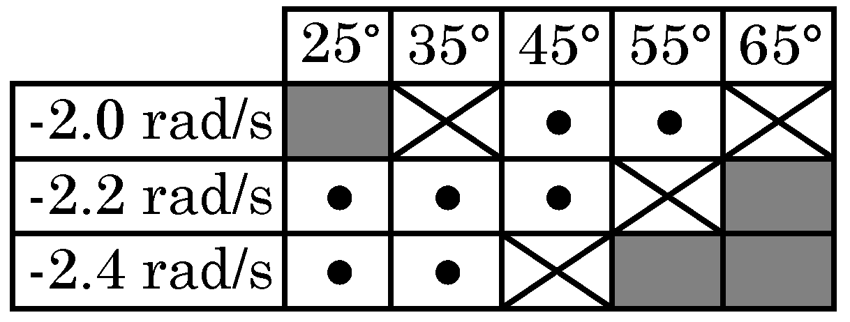
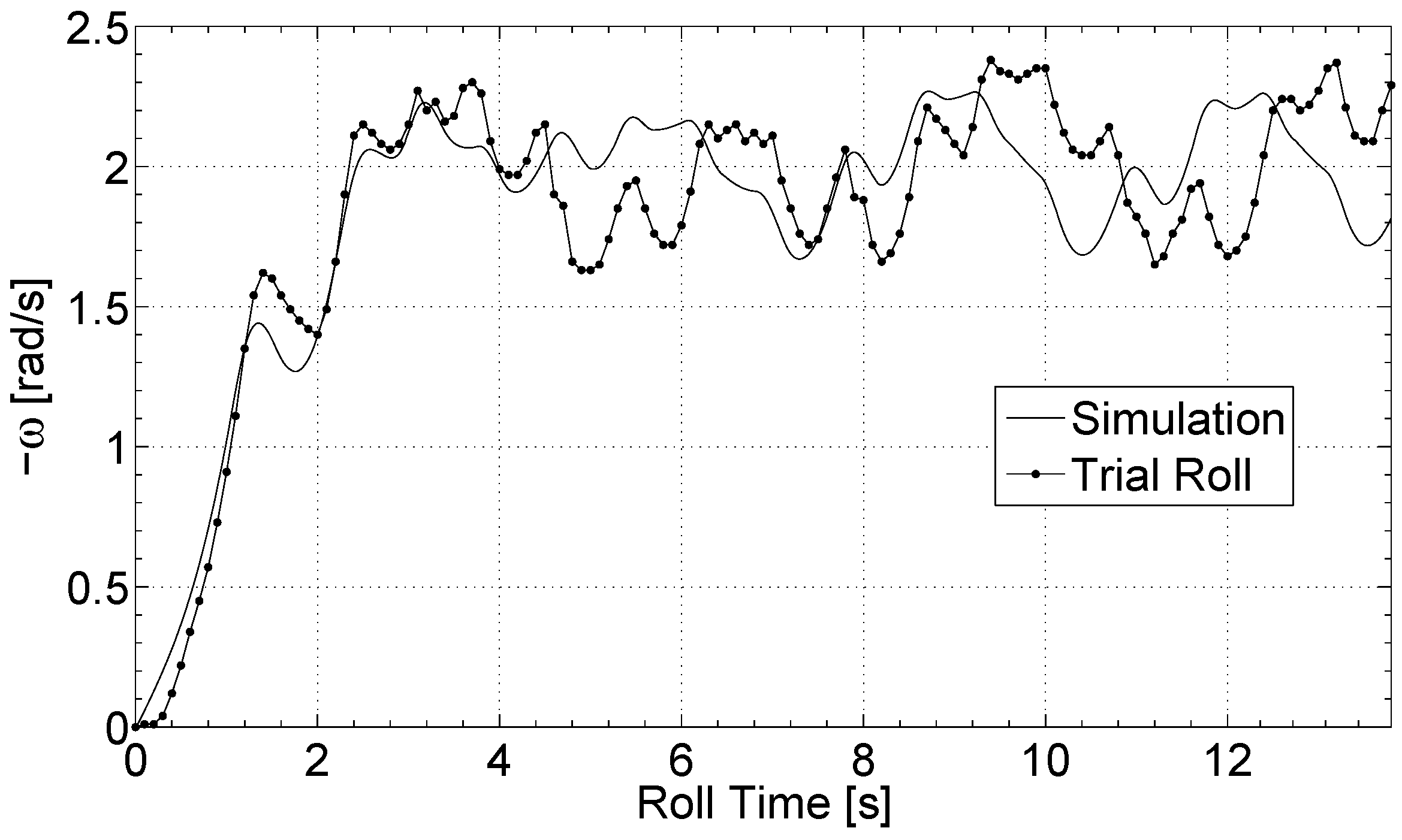
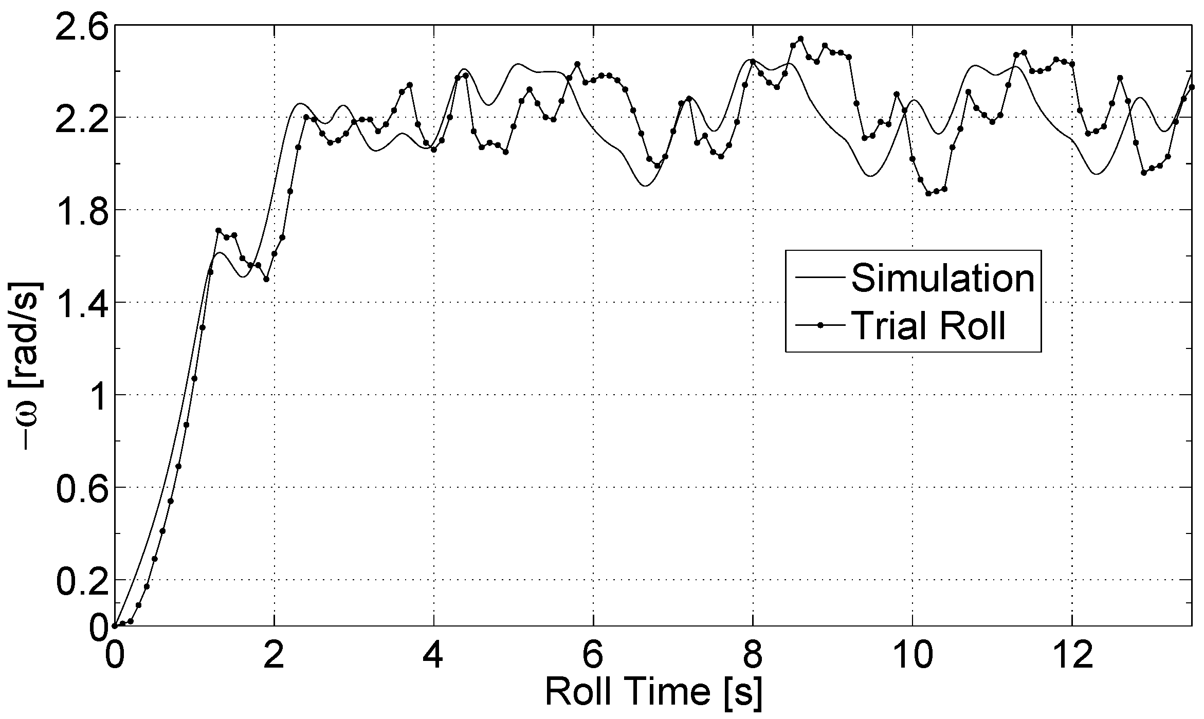
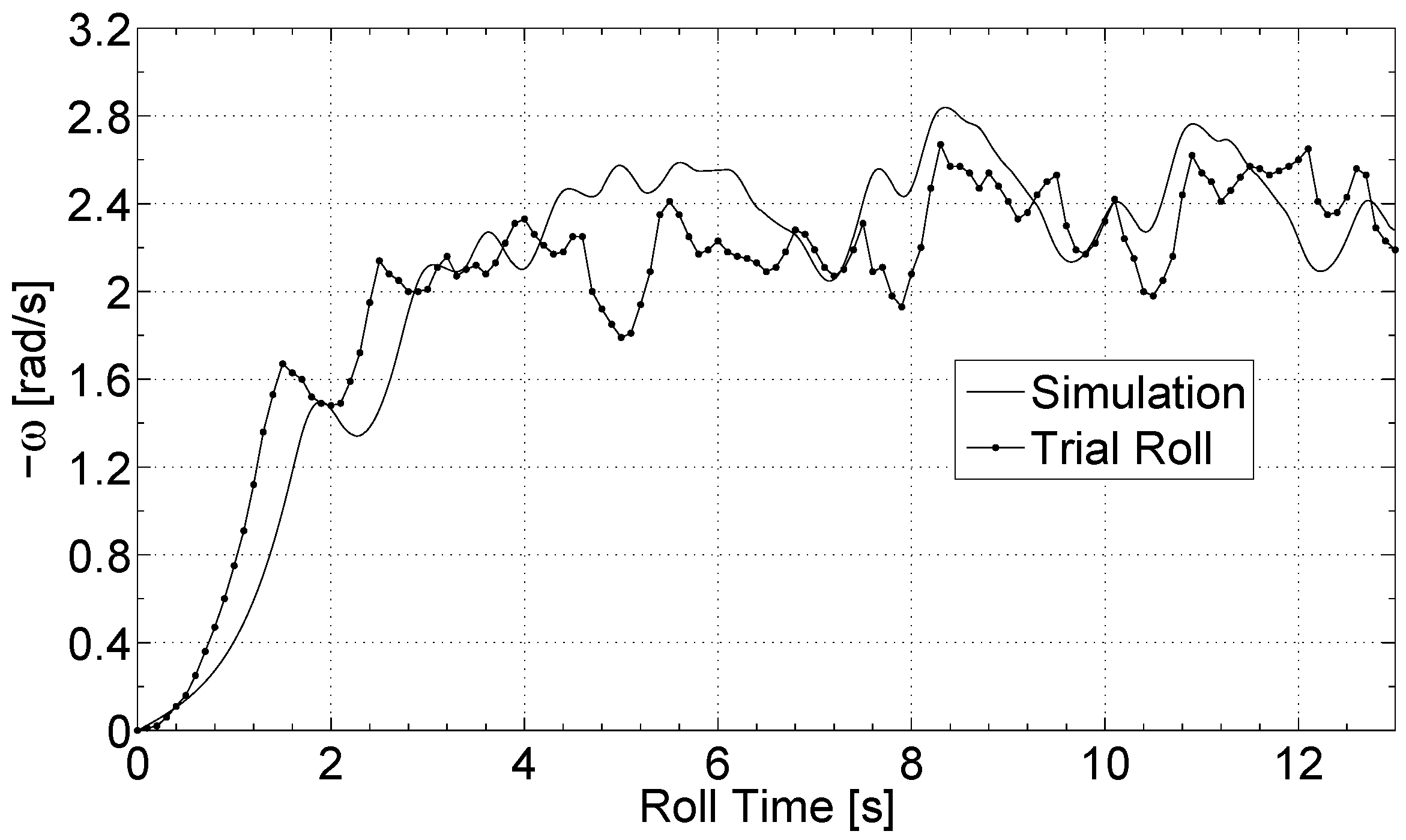
Figure 7 is a tabulated summary of results from the trial roll experiment, in which superior values of are identified for the various values of . In addition, the simulation program is configured to perform three rolls of the robot. Each of the simulated rolls has a set of initial conditions and control constants that are identical to a trial roll conducted in the experiment. Roll 1 is from Problem 1 with , , and rad/s. Roll 2 is from Problem 2 with , , and rad/s. Roll 3 is from Problem 3 with , , and rad/s. By design, the rolls have desired angular velocities and trigger angles whose collective values span the ranges of these parameters tested in the experiment. The simulation program is configured to output locomotion parameters, including , at 10 millisecond intervals of roll time for the simulated trial rolls. Output values of angular velocity from the simulated rolls are gathered and plotted along with angular velocity from actual trial rolls, and the resulting comparison plots for Rolls 1–3 are included in Figure 8, Figure 9 and Figure 10.
4. Discussion
The most interesting takeaway from the research documented herein is that, for each tested in the experiment, there exists a range of two or three values of that are determined to be superior in terms of energy economy of robot locomotion. When is decreased relative to this range, so that actuation is triggered with less tilt of the triggering axis with respect to the vertical, energy economy of robot locomotion is observed to decrease; and when is increased relative to this range, so that actuation is triggered with more tilt of the triggering axis, energy economy of robot locomotion is again observed to decrease. There is therefore an optimal range of with regard to energy economy for each tested in the experiment. Furthermore, results of the experiment reveal that as desired angular velocity of the robot is changed, the optimal range of changes as well. In general, this optimal range shifts downward (i.e., less tilt of the triggering axis) as velocity magnitude of the robot is increased from rad/s to rad/s.
In order to understand the existence of this range of and why it shifts with robot speed, recall that the robot control system works by repeatedly morphing outer surface shape in order to change location of the normal force relative to the robot center of mass. In this way, the control system ensures that the normal force is most often located to the left of the center of mass during stable locomotion of the robot, causing input torque to be applied in a clockwise sense to drive the robot along X in the positive direction and to follow, on average, a desired angular velocity. However, upon careful scrutiny of controlled motion of the robot, it is apparent that the control system, which actuates shape change at most four times per revolution of the robot, has mixed consequences—that is, the control system speeds up the robot, but it sometimes slows it down as well.
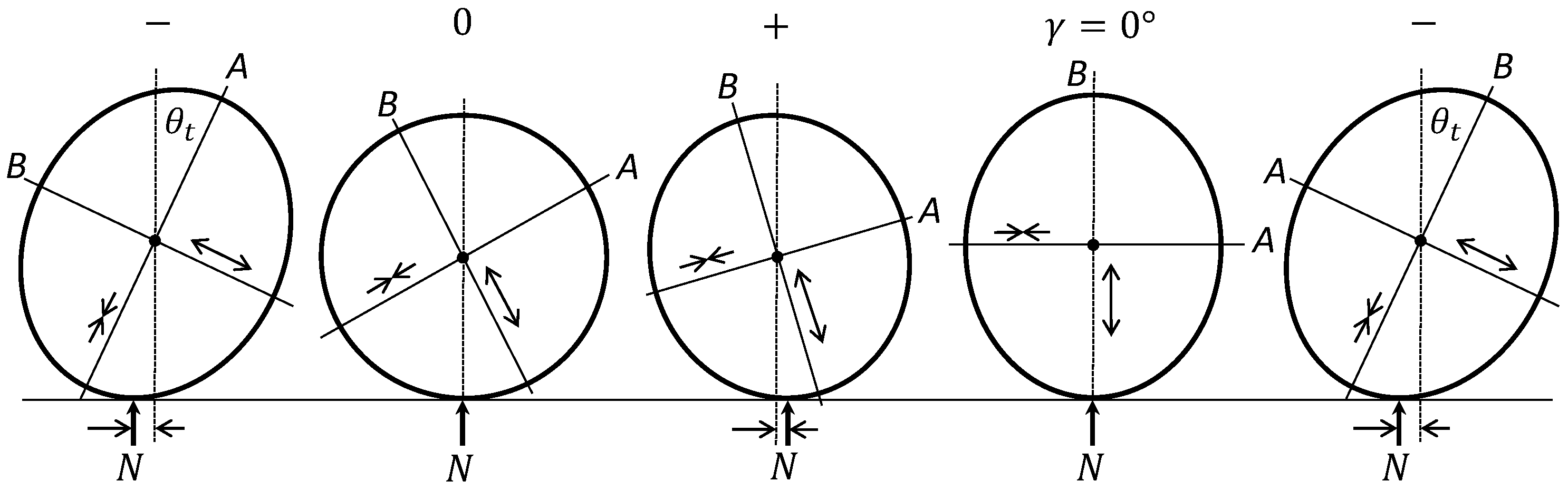
Imagine the roll scenario illustrated in Figure 11 where roll instances are arranged chronologically from left to right. In this scenario, is set below the optimal range for rad/s, meaning that actuation occurs “early" in the cycle when . At the first instance in the scenario, A has just swept past the trigger angle, and shape change actuation has begun. The moment arm, , is negative because oblongness of the outer surface, combined with the slight tilt of the robot, place the touchpoint to the left of the robot center of mass. With a negative moment arm, is clockwise in the first instance, and the robot speeds up as a result. Because shape change actuation occurs early in this scenario, the outer surface of the robot actuates to the circular configuration, as in the second instance in Figure 11, before A crosses the horizontal orientation. In the circular configuration, is zero. At instance three, the robot has become oblong about B, and A still has not crossed the horizontal, so that has become positive and is now counterclockwise, and the robot briefly undergoes inadvertent braking. At instance four, A has rotated into the horizontal, at which point and inevitably become zero again, and the scenario subsequently repeats with A and B in switched positions by the fifth instance.
A symbolic representation is introduced to characterize the input torque pattern on the robot in this early actuation scenario, wherein a plus sign is used to represent counterclockwise torque on the robot, and a negative sign is used to represent clockwise torque. The “0” digit is used to represent zero torque on the robot, and the expression, , is used to represent the instance when A or B is oriented horizontally, when gamma and are both zero. Starting at the first instance and using this symbolic representation, the pattern displayed by the early actuation scenario is: −, 0, +, , −, 0, +, , −, etc. A marked feature of this actuation pattern is the sequence: +, , −; that is to say, when , torque on the robot is changing from counterclockwise to clockwise.
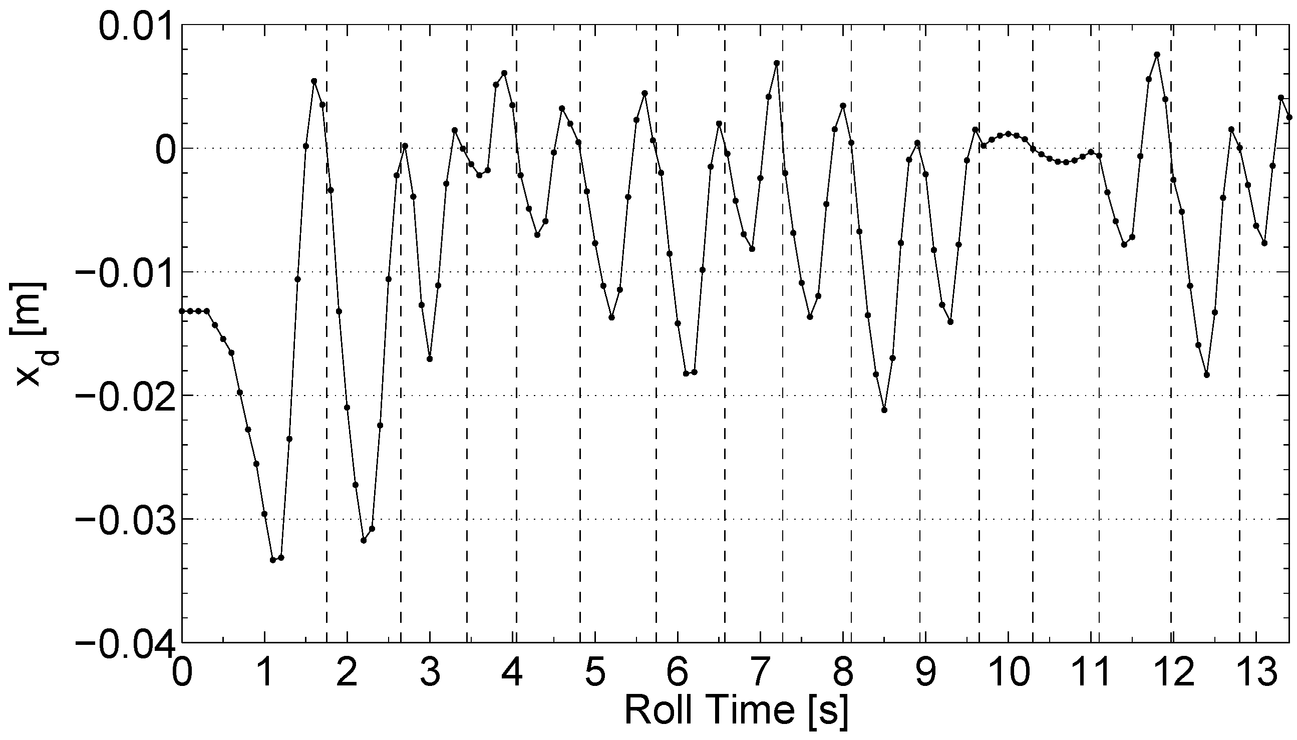
For the purpose of learning if the robot exhibits the early actuation pattern during actual locomotion, four individual trial rolls from Problem 1, one for each viable value of , are chosen and investigated. The values of for the chosen rolls are consistent with average values of the corresponding populations. The four trial rolls are referred as Roll A, Roll B, Roll C and Roll D, respectively corresponding to = 35°, 45°, 55°, and 65°. Equation (14) is used with reported roll data to compute at every tenth of a second for each roll. In Figure 12, computed values of are plotted versus roll time for Roll A. Dashed, vertical lines in the graph represent approximate moments during the roll when . A plot of angular velocity versus roll time for Roll A is also included in Figure 13.
The plot of in Figure 12 reveals that is frequently positive, which means the rolling robot experiences repeated inadvertent braking during steady state. These times are relatively short-lived, and the magnitude of during inadvertent braking is generally smaller than when is negative, and this result means driving torque supplies more energy to the robot than does inadvertent braking, which is expected, since the purpose and demonstrated outcome of the control system is to maintain forward motion of the robot. The actuation pattern for Roll A is clearly that of early actuation. The graph in Figure 12 shows 13 times at which , and at ten or more of these times, the pattern is: +, , −, which is that of early actuation. For Roll A, is set to 35°, which is below the optimal range of identified for rad/s, so it is not surprising that the early actuation pattern would manifest here.
The early actuation pattern manifested during Roll A sheds light on why there is a lower limit on optimality of in Problem 1. When is set too low (actuation triggering is too early), the robot is prone to inadvertent braking, potentially at every cycle. Notice from Figure 12 that, when braking occurs, it is not always beneficial. That is to say, the robot often works against itself with considerable energy during the roll, slowing itself down when it is already going too slow. A good example occurs at roughly 5.5 s. At this time, the robot is already rotating too slowly (see Figure 13) relative to the desired velocity magnitude when inadvertent braking comes on at 5.8 s and slows down the robot even more. Consequently, the linear actuator is subsequently forced by the control system to move at a large magnitude to create driving torque in order to speed up the robot and maintain the desired velocity. A similar thing happens between 11 and 12 s. With so much ill-timed braking, it is understandable why Roll A with is not optimal in terms of energy economy.
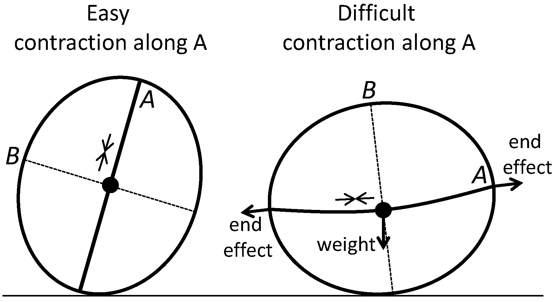
Similar investigations into Rolls B, C and D reveal that there is nothing about the respective plots of that points to why robot locomotion during Rolls B and C are relatively economical compared to Roll D, as is established by the results of the experiment (Figure 7). This absence of contrast leads one to believe there is a factor separate from actuation patterning that affects energy economy of rolls in Problem 1. In an effort to identify this factor, reported information from Roll D is scrutinized, and it is noticed that high energy consumption rates during Roll D correspond to periods of actuation when A is the trigger axis. With this correspondence in mind, the average rate of energy consumption by the servo motor is calculated for actuation when A is the trigger axis, and it is found to be higher, on average, than when B is the trigger axis or during periods when the actuator is holding a constant. The reason higher trigger angle values are associated with greater actuation burden is that deformation of the outer surface is greater during such actuation moves, resulting in outwardly directed end effects that pull on the actuator and resist contraction. In contrast, when orientation of A during actuation is closer to the vertical, there is less bending of the telescoping columns and hence less friction; furthermore, gravity actually helps the actuator contract when it is orientated in an upright orientation. The effect of orientation of A on actuation burden is illustrated in Figure 14.
With these insights, energy economy results from Problem 1 can now be understood as stemming from a combination of inadvertent braking and actuation burden. To summarize, at one extreme when is set low at 35°, angular velocity of the robot, which is rad/s on average, is small enough in magnitude so the actuating outer surface often attains the circular configuration before . In other words, the robot exhibits the early actuation pattern, as illustrated in Figure 11, in which it frequently undergoes inadvertent braking and works against itself. For this reason, robot locomotion has relatively low energy economy for . At the other extreme, when is set high at 65°, actuation becomes increasingly burdensome due to the effects of gravity and bending of the outer surface, thereby nullifying gains in economy that might otherwise be had. In between 35° and 65°, there is an optimal range where is high enough for the robot to largely avoid the averse early actuation pattern, yet low enough so that actuation burden does not greatly hinder the system. The same explanation given here for energy economy in Problem 1 applies to trial rolls in Problems 2 and 3, but with the difference that at higher rotation speeds, actuation burden is shifted downward on relative to Problem 1, so that = 55° and 45° are rendered least economical for Problems 2 and 3, respectively, while the lower trigger angles tested for each of these problems are most economical.
5. Conclusions
A rolling robot has been developed that generates torque by changing shape of its elliptical outer surface, which is flexible and can be morphed to retain oblongness about one of two notional, elliptical axes that are fixed to the robot and roll with it. The robot has been equipped with a sensing/control system by which it measures its angular position and angular velocity, computes error with respect to a desired step velocity profile, and changes the shape of its outer surface accordingly. Shape change actuation occurs four times per revolution, whenever an elliptical axis rotates past a predetermined trigger angle. The robot has demonstrated stability during roll tests, in the sense that it was able to quickly reach a constant desired angular velocity and remain close to it thereafter.
A series of trial rolls of the robot were performed using various trigger angles, while energy consumed by the servo motor was measured and used to calculate energy economy for each roll. Results of this experiment showed that, depending on the velocity of the robot, there exists a range of trigger angle values that are superior in terms of energy economy. This region of optimality on trigger angle generally shifts towards the vertical as desired angular velocity is increased. In search for an explanation, it was found that economical trial rolls featured a synchronicity of actuation timing and angular velocity, wherein the robot avoided agents of inefficiency that slowed the robot or burdened the servo motor. At higher magnitude angular velocities of the robot, actuations triggered at sufficiently small tilt angles preserved the synchronicity.
A mathematical model was developed for the robot that included bending of the outer surface and rolling resistance torque. Based on the model, a computer program was developed that simulated locomotion of the robot and was used to plot various motion parameters such as angular velocity and roll distance versus roll time. The program was configured to perform three simulation runs corresponding to actual trial rolls of the robot. Angular velocity from the simulations was compared to measured values from actual trial rolls, and the model was found to be significantly accurate.
In future research efforts, the authors would like to investigate the possibility of making an extraction of the OSU Roller with an outer surface that is bigger or smaller in circumference than the OSU Roller. Having developed a mathematical model of the robot, the effects on performance of such changes in size could easily be investigated in theory. In addition, perhaps future shape changing rolling robots could be constructed of adaptive materials such as Nitinol, pneumatic muscles, or a thermally tunable foam that acts as frame, wheel and actuator all-in-one. Imagining such extractions, which are presumably not too far off in the future, highlights how shape changing rollers have the potential to be simple, ultralightweight, efficient robots for use in various applications, including space exploration [25].
Author Contributions
E.G. contributed to the design of the robot energy sensor and revised the paper; J.D.J. contributed to the design of the experiment, interpreted data, and performed substantial revisions to the paper; M.G.P. designed and manufactured the robot, programmed the robot, contributed to the design of the experiment, interpreted data, performed the experiment, developed the mathematical model, and wrote the paper.
Funding
This research was funded in part by the Unmanned Systems Research Institute at Oklahoma State University.
Acknowledgments
The authors would like to acknowledge helpful discussions with Russ Rhinehart and donations of materials for the robot by Slate Rehm, Darby Rehm, and Chanten Rehm.
Conflicts of Interest
The authors declare no conflict of interest.
References
- McKerrow, P.J. Introduction to Robotics; Chapter Components and Subsystems; Addison Wesley Publishing Company: Sydney, Australia, 1991; p. 57. [Google Scholar]
- Bogue, R. Shape Changing Self-Reconfiguring Robots. Ind. Robot Int. J. 2015, 42, 290–295. [Google Scholar] [CrossRef]
- Watanabe, W.; Sato, T.; Ishiguro, A. A Fully Decentralized Control of a Serpentine Robot Based on the Discrepancy between Body, Brain and Environment. In Proceedings of the 2009 IEEE/RSJ International Conference on Intelligent Robots and Systems, St. Louis, MO, USA, 10–15 October 2009; pp. 2421–2426. [Google Scholar]
- Armour, R.; Vincent, F. Rolling in Nature and Robotics: A Review. J. Bionic Eng. 2006, 3, 195–208. [Google Scholar] [CrossRef]
- Sastra, J.; Chitta, S.; Yim, M. Dynamic Rolling for a Modular Loop Robot. Int. J. Robot. Res. 2009, 28, 758–773. [Google Scholar] [CrossRef] [Green Version]
- Sugiyama, Y.; Hirai, S. Crawling and Jumping by a Deformable Robot. Int. J. Robot. Res. 2006, 25, 603–620. [Google Scholar] [CrossRef]
- Matsuda, T.; Murata, S. Stiffness Control—Locomotion of Closed Link Robot with Mechanical Stiffness. In Proceedings of the 2006 IEEE International Conference on Robotics and Automation, Orlando, FL, USA, 15–19 May 2006; pp. 1491–1498. [Google Scholar]
- Tedrake, R. Underactuated Robotics: Algorithms for Walking, Running, Swimming, Flying and Manipulation (Course Notes for MIT 6.832). 2016. Available online: http://underactuated.mit.edu (accessed on 8 March 2017).
- Mochon, S.; McMahon, T.A. Ballistic Walking. J. Biomech. 1980, 13, 49–57. [Google Scholar] [CrossRef]
- McGeer, T. Passive Dynamic Walking. Int. J. Rob. Res. 1990, 9, 62–82. [Google Scholar] [CrossRef]
- Tavakoli, A. Gravity powered locomotion and active control of three mass system. In Proceedings of the ASME 2010 Dynamic Systems and Control Conference, Cambridge, MA, USA, 12–15 September 2010; pp. 141–148. [Google Scholar]
- Chiu, H.C.; Rubenstein, M.; Shen, W.M. Multifunctional SuperBot with Rolling Track Configuration. In Proceedings of the 2007 IEEE/RSJ International Conference on Intelligent Robots and Systems, San Diego, CA, USA, 29 October–2 November 2007. [Google Scholar]
- Mellinger, D.; Kumar, V.; Yim, M. Control of Locomotion with with Shape-Changing Wheels. In Proceedings of the 2009 IEEE International Conference on Robotics and Automation, Kobe, Japan, 12–17 May 2009; pp. 1750–1755. [Google Scholar]
- Melo, K.; Velasco, A.; Parra, C. Motion Analysis of an Ellipsoidal Kinematic Closed Chain. In Proceedings of the 2011 IEEE IX Latin American Robotics Symposium and IEEE Colombian Conference on Automatic Control, Bogota, Colombia, 1–4 October 2011. [Google Scholar]
- Puopolo, M.G.; Jacob, J.D. Velocity control of a cylindrical rolling robot by shape changing. Adv. Robot. 2016, 30, 1484–1494. [Google Scholar] [CrossRef]
- Chitode, J.; Bakshi, U. Power Devices and Machines; Technical Publications Pune: Maharashtra, India, 2009; pp. 7.20–7.23. [Google Scholar]
- Serway, R.A. Physics for Scientist and Engineers, 3rd ed.; Saunders College Publishing: Philadelphia, PA, USA, 1990; Chapters 7, 27; pp. 152–173, 740–760. [Google Scholar]
- Chandrupatla, T.R.; Osler, T.J. The Perimeter of an Ellipse. Math. Sci. 2010, 35, 122–131. [Google Scholar]
- Hibbeler, R. Dynamics, 12th ed.; Chapter Kinetics of a Particle: Impulse and Momentum; Prentice Hall: Upper Saddle River, NJ, USA, 2010; pp. 262–297. [Google Scholar]
- Pal, S. Numerical Methods; Oxford University Press: Oxford, UK, 2013; Chapters 14, 15; pp. 439–440, 522–538. [Google Scholar]
- Savitch, W. Absolute C++; Chapter C++ Basics; Pearson: Boston, MA, USA, 2013; p. 4. [Google Scholar]
- Chou, Y. Statistical Analysis; Chapter Queing Theory and Monte Carlo Simulation; Holt, Rinehart & Winston of Canada: Toronto, ON, Canada, 1969; pp. 720–730. [Google Scholar]
- Pett, M.A. Nonparametric Statistics for Health Care Research; Chapter Addressing Differences Among Groups; Sage Publications: Thousand Oaks, CA, USA, 1997; pp. 204–211. [Google Scholar]
- Puopolo, M.G. Locomotion of a Cylindrical Rolling Robot with a Shape Changing Outer Surface. Ph.D. Thesis, Oklahoma State University, St. Walter, OK, USA, 2017. [Google Scholar]
- Antol, J.; Calhoun, P. Low Cost Mars Surface Exploration: The Mars Tumbleweed; Technical Report NASA/TM-2003-212411; National Aeronautics and Space Administration: Washington, DC, USA, 2003. [Google Scholar]
Figure 1.
The OSU Roller has a mass of 0.950 kg with a perimeter of 2.095 m.

Figure 2.
The robot model includes affects of bending and has three forces acting on the robot: weight, normal force and traction. The model also includes torque caused by rolling resistance.
Figure 2.
The robot model includes affects of bending and has three forces acting on the robot: weight, normal force and traction. The model also includes torque caused by rolling resistance.

Figure 3.
The moment, , causes a torque imbalance about the robot center of mass, affecting roll dynamics of the robot.
Figure 3.
The moment, , causes a torque imbalance about the robot center of mass, affecting roll dynamics of the robot.

Figure 4.
An example of stable locomotion of the robot for rad/s. Angular velocity rises quickly to the desired level and remains close to it thereafter.
Figure 4.
An example of stable locomotion of the robot for rad/s. Angular velocity rises quickly to the desired level and remains close to it thereafter.

Figure 5.
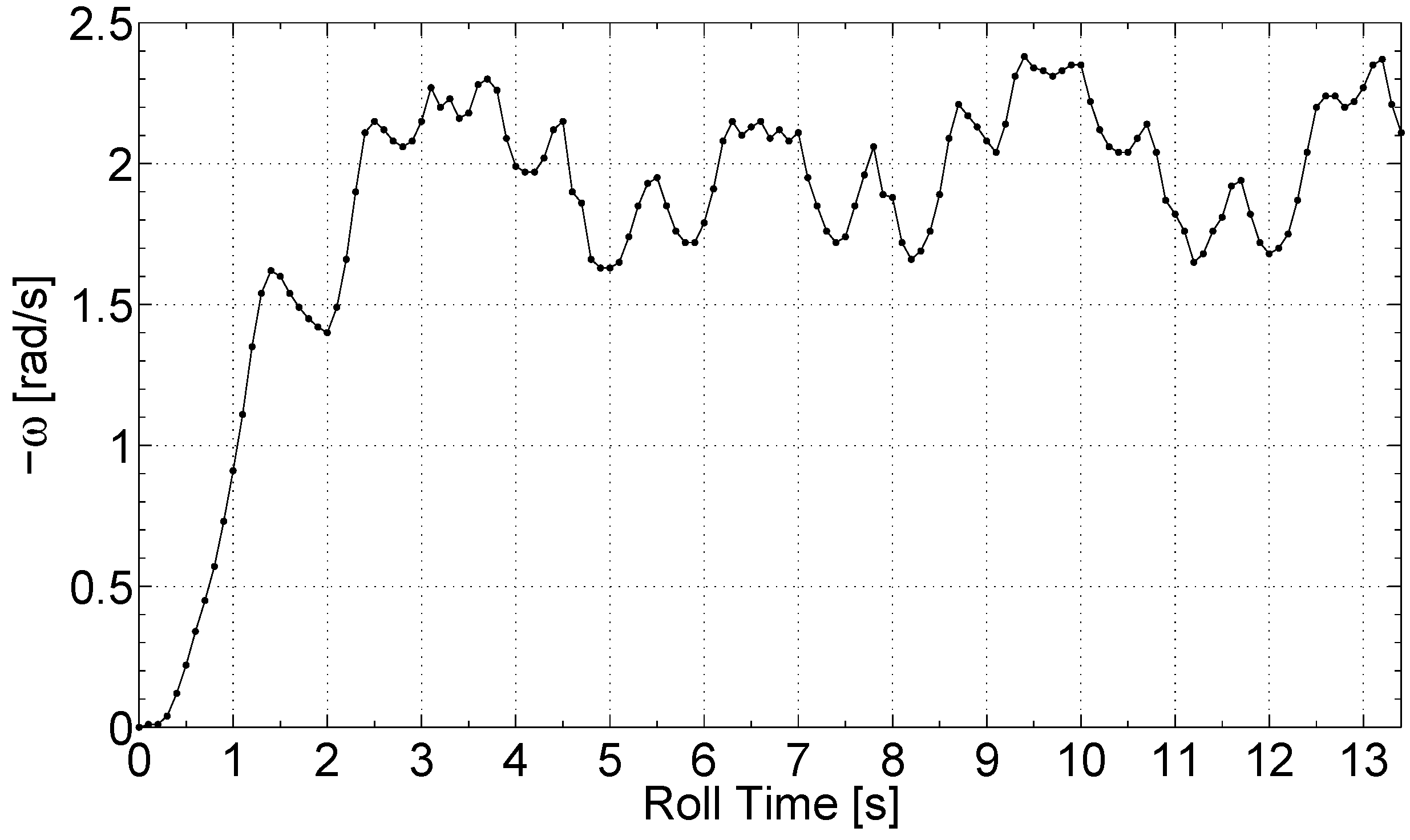
An example of unstable locomotion for the robot for rad/s. Average angular velocity dips far below the desired level during the latter half of the trial roll.
Figure 5.
An example of unstable locomotion for the robot for rad/s. Average angular velocity dips far below the desired level during the latter half of the trial roll.

Figure 6.
Roll track for the robot is a flat and level section of laminate flooring installed on concrete.
Figure 6.
Roll track for the robot is a flat and level section of laminate flooring installed on concrete.

Figure 7.
Cells with a dot signify values of that are superior in terms of energy economy of robot locomotion. Gray cells signify values of that cause instability, and cells with a cross-out signify inferior values of .
Figure 7.
Cells with a dot signify values of that are superior in terms of energy economy of robot locomotion. Gray cells signify values of that cause instability, and cells with a cross-out signify inferior values of .

Figure 8.
Robot angular velocity from simulation and from trial roll are plotted versus roll time for Roll 1, in which rad/s.
Figure 8.
Robot angular velocity from simulation and from trial roll are plotted versus roll time for Roll 1, in which rad/s.

Figure 9.
Robot angular velocity from simulation and from trial roll are plotted versus roll time for Roll 2, in which rad/s.
Figure 9.
Robot angular velocity from simulation and from trial roll are plotted versus roll time for Roll 2, in which rad/s.

Figure 10.
Robot angular velocity from simulation and from trial roll are plotted versus roll time for Roll 3, in which rad/s.
Figure 10.
Robot angular velocity from simulation and from trial roll are plotted versus roll time for Roll 3, in which rad/s.

Figure 11.
When the robot exhibits the early actuation pattern, inadvertent braking occurs before the robot has reached the orientation.
Figure 11.
When the robot exhibits the early actuation pattern, inadvertent braking occurs before the robot has reached the orientation.

Figure 12.
For Roll A, the robot exhibits the early actuation pattern, in which inadvertent braking (when is positive) causes the roll to have relatively low energy economy.
Figure 12.
For Roll A, the robot exhibits the early actuation pattern, in which inadvertent braking (when is positive) causes the roll to have relatively low energy economy.

Figure 13.
Angular velocity of the robot for Roll A, a roll with relatively low energy economy. At times, the robot slows itself down when it is already going too slow relative to the desired velocity of −2.0 rad/s.
Figure 13.
Angular velocity of the robot for Roll A, a roll with relatively low energy economy. At times, the robot slows itself down when it is already going too slow relative to the desired velocity of −2.0 rad/s.

Figure 14.
When A is oriented nearly vertically, gravity makes contraction “easy” for the linear actuator. When oriented horizontally, weight and outwardly directed end effects on the linear actuator make contraction “difficult”.
Figure 14.
When A is oriented nearly vertically, gravity makes contraction “easy” for the linear actuator. When oriented horizontally, weight and outwardly directed end effects on the linear actuator make contraction “difficult”.

© 2018 by the authors. Licensee MDPI, Basel, Switzerland. This article is an open access article distributed under the terms and conditions of the Creative Commons Attribution (CC BY) license (http://creativecommons.org/licenses/by/4.0/).
Share and Cite
MDPI and ACS Style
Puopolo, M.G.; Jacob, J.D.; Gabino, E. Locomotion of a Cylindrical Rolling Robot with a Shape Changing Outer Surface. Robotics 2018, 7, 52. https://doi.org/10.3390/robotics7030052
AMA Style
Puopolo MG, Jacob JD, Gabino E. Locomotion of a Cylindrical Rolling Robot with a Shape Changing Outer Surface. Robotics. 2018; 7(3):52. https://doi.org/10.3390/robotics7030052
Chicago/Turabian StylePuopolo, Michael G., Jamey D. Jacob, and Emilio Gabino. 2018. "Locomotion of a Cylindrical Rolling Robot with a Shape Changing Outer Surface" Robotics 7, no. 3: 52. https://doi.org/10.3390/robotics7030052
Note that from the first issue of 2016, this journal uses article numbers instead of page numbers. See further details here.