
Planning the Minimum Time and Optimal Survey Trajectory for Autonomous Underwater Vehicles in Uncertain Current

Abstract
:1. Introduction

2. Modeling Assumptions

3. Analytical Approach to an Extremal Path
Adjoint Variables: Effect of Current
4. Numerical Approach to the Optimum Path
4.1. The Minimum Time Problem

| Current/Path | 1 | 2 | 3 | 4 | 5 |
|---|---|---|---|---|---|
| 1 | 798 | 804 | 812 | 838 | 920 |
| 2 | 821 | 817 | 824 | 849 | 907 |
| 3 | 873 | 864 | 858 | 878 | 918 |
| 4 | 998 | 987 | 943 | 930 | 955 |
| 5 | 1871 | 1460 | 1225 | 1087 | 1039 |
| Average | 1072 | 986 | 932 | 916 | 948 |
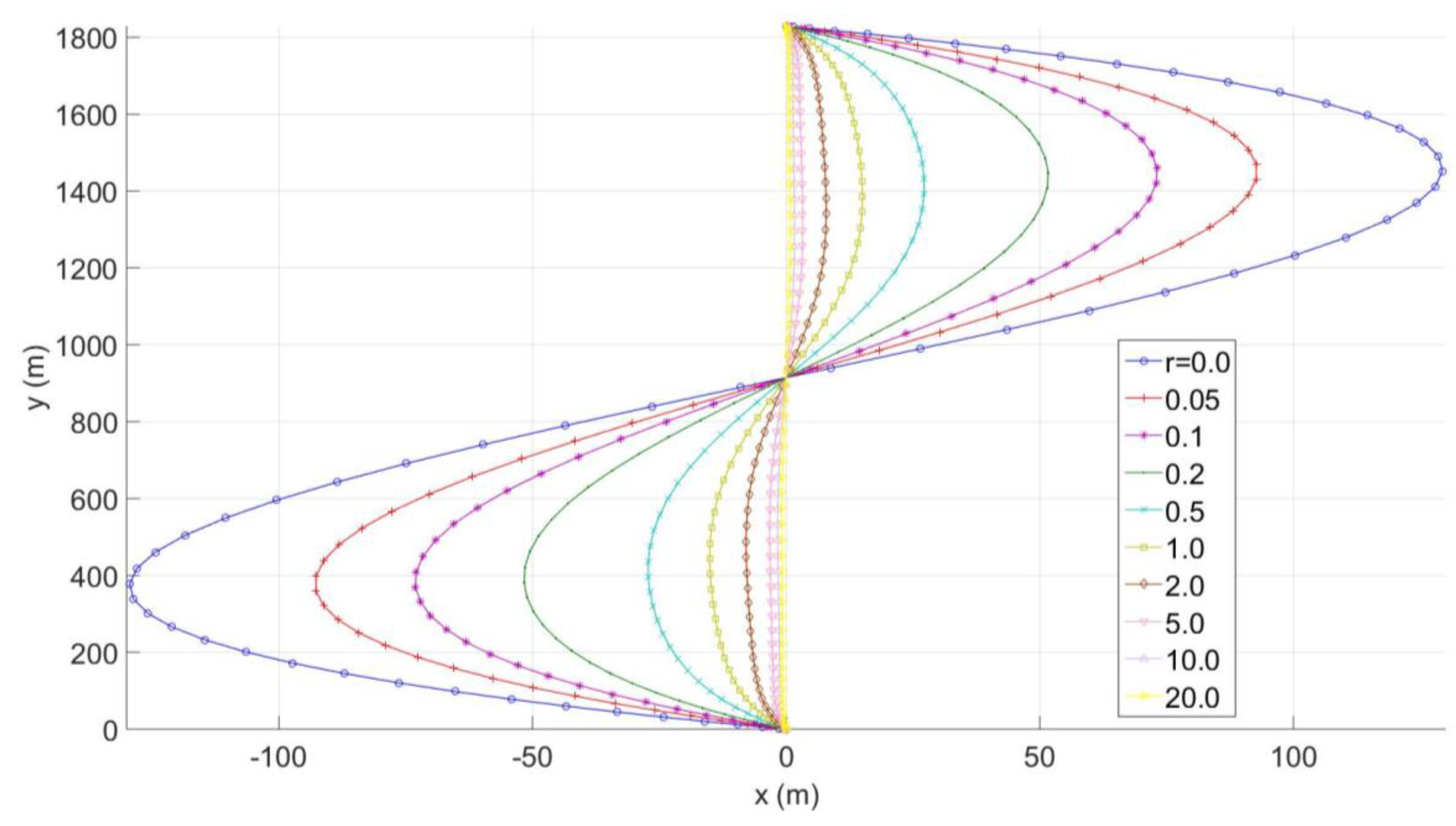
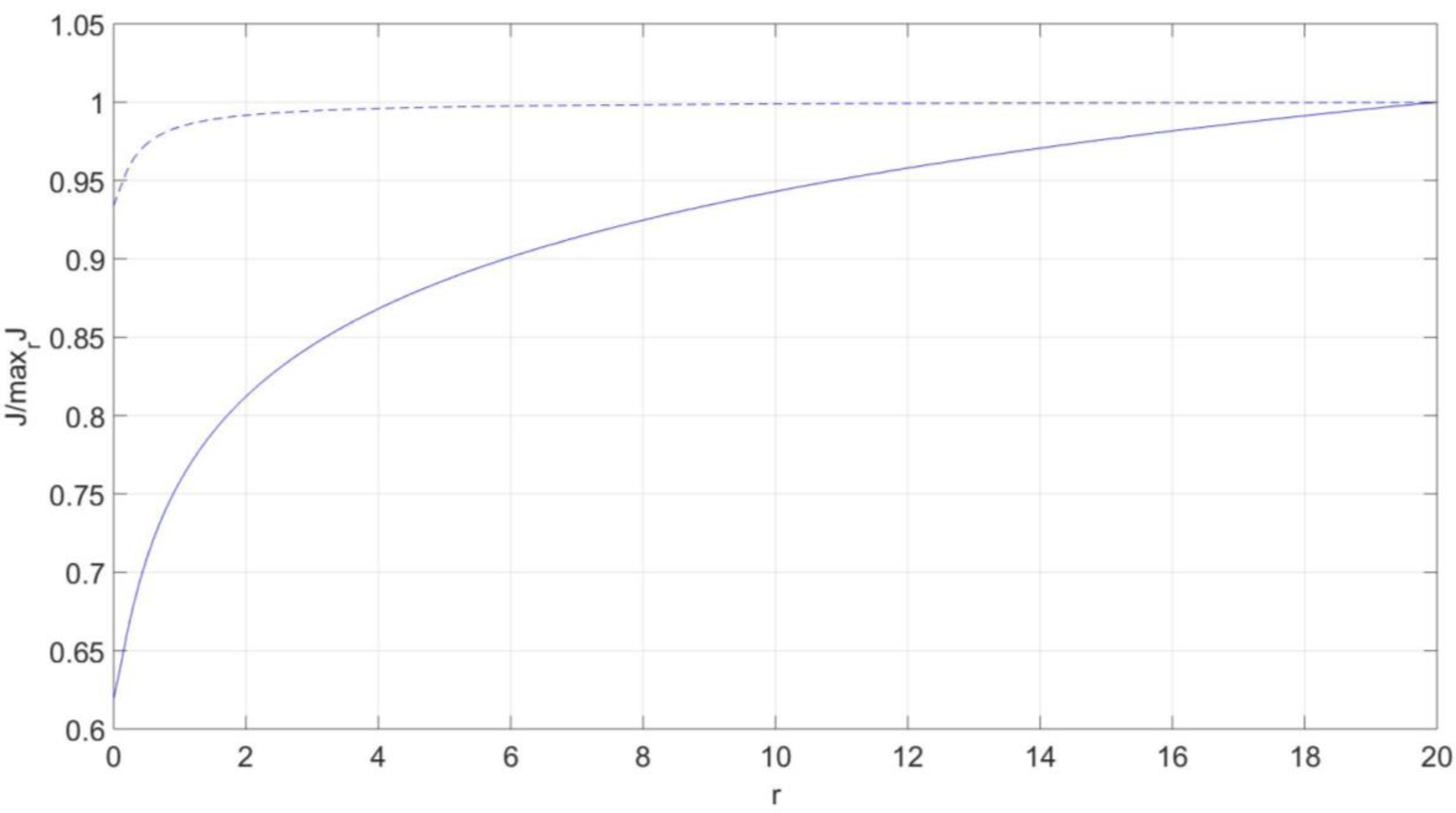
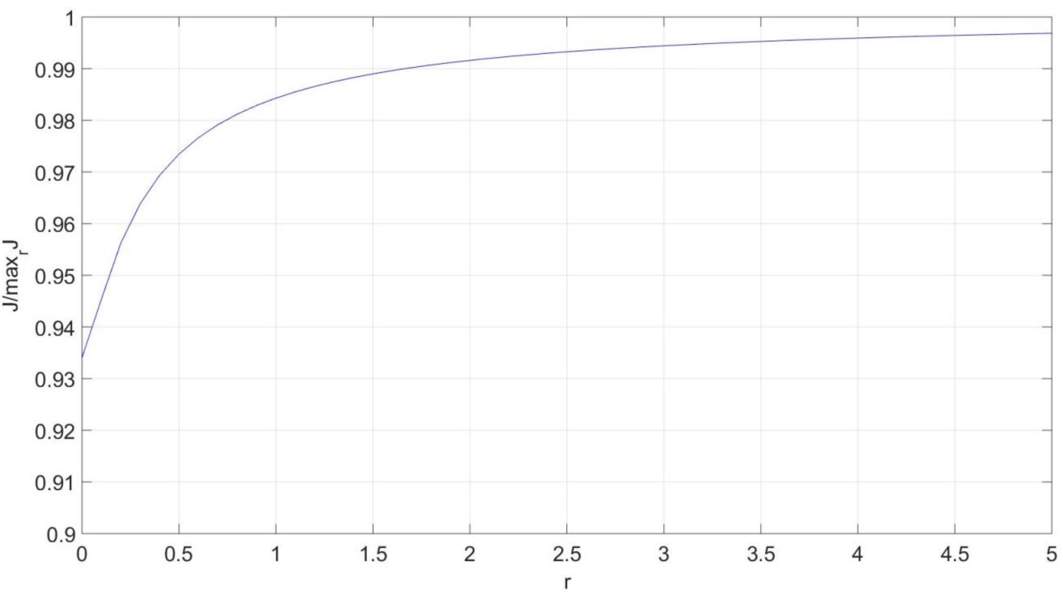
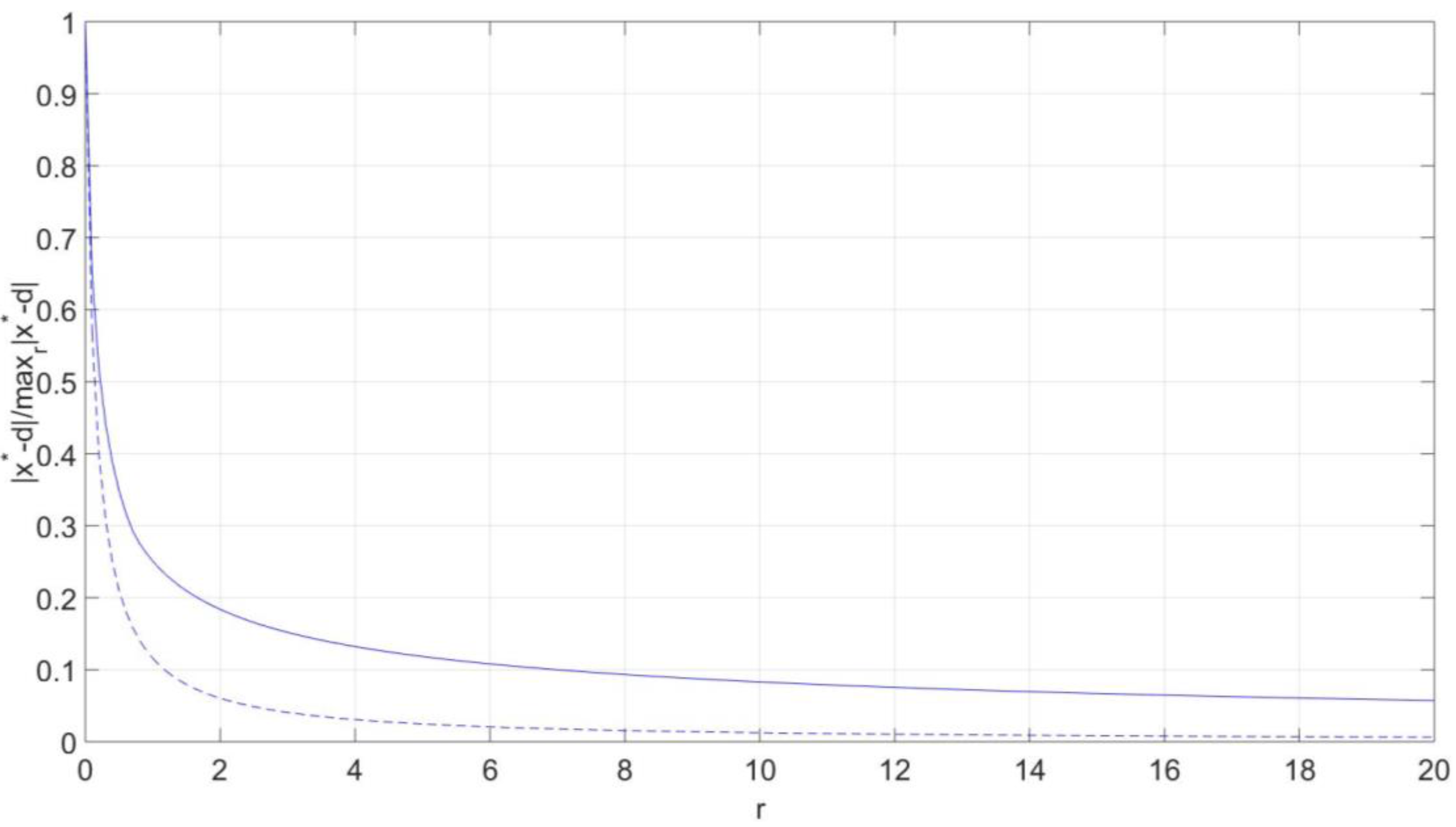
4.2. Time vs. Accuracy
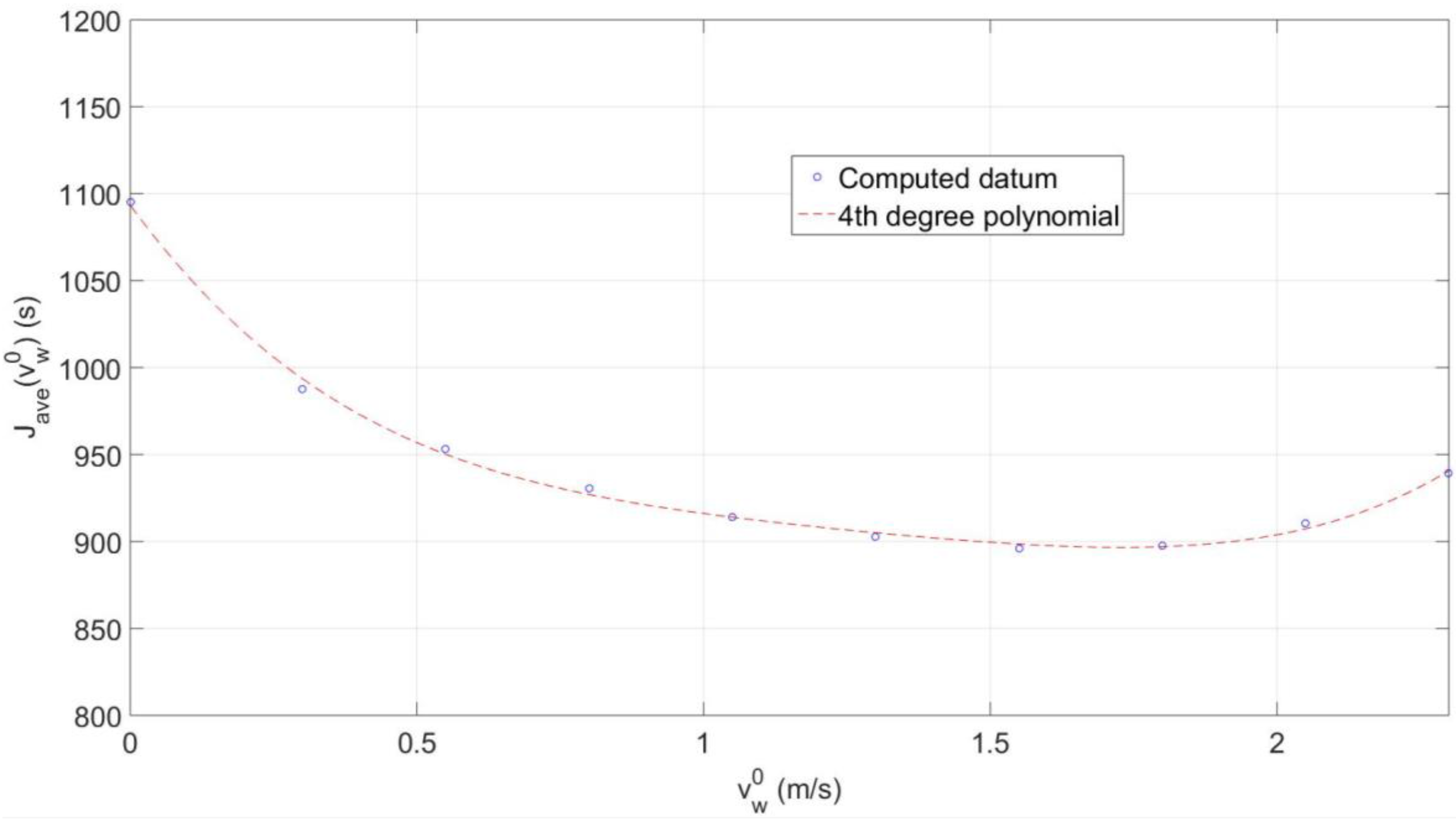
4.3. Actual Current Coincides with Assumed

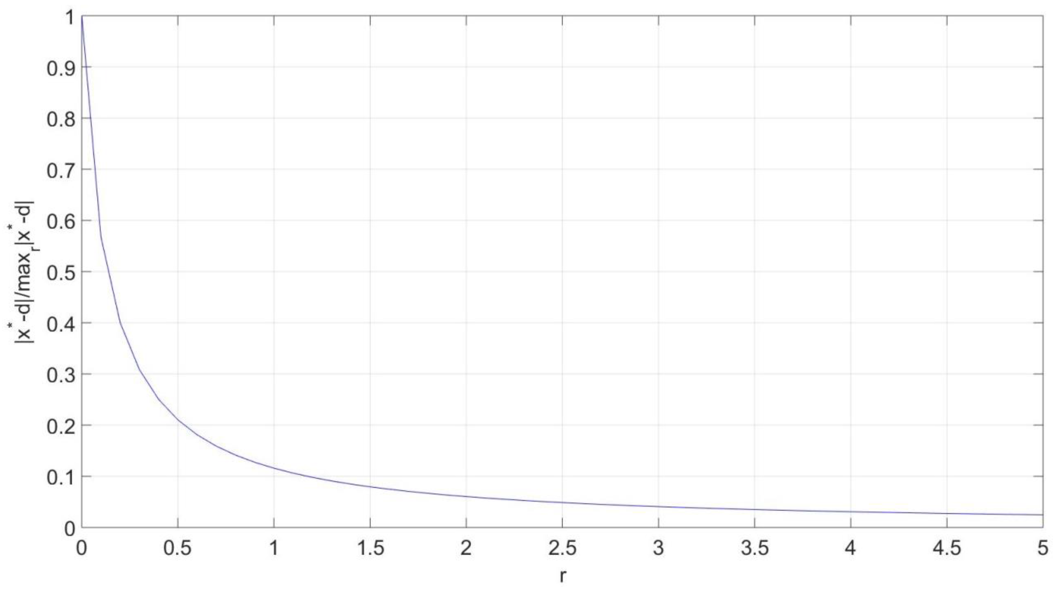
4.4. Actual Current Differs from Assumed

5. Conclusions
Conflicts of Interest
References
- REMUS 100. Available online: http://www.km.kongsberg.com (accessed on 23 March 2014).
- Hurni, M.A.; Kiriakidis, K.; Nicholson, J.W. Planning the Minimum Time Course for Autonomous Underwater Vehicle in Uncertain Current. In Proceedings of the ASME Dynamic Systems and Control Conference, Palo Alto, CA, USA, 21–23 October 2013.
- Bryson, A.E.; Ho, Y.C. Applied Optimal Control; Hemisphere Publishing Corporation: New York, NY, USA, 1975. [Google Scholar]
- Petres, C.; Pailhas, Y.; Patron, P.; Petillot, Y.; Evans, J.; Lane, D. Path planning for autonomous underwater vehicles. IEEE Trans. Robot. 2007, 23, 331–341. [Google Scholar] [CrossRef]
- Tinka, A.; Diemer, S.; Madureira, L.; Marques, E.B.; de Sousa, J.B.; Martins, R.; Pinto, J.; da Silva, J.E.; Sousa, A.; Saint-Pierre, P.; et al. Viability-based computation of spatially constrained minimum time trajectories for an autonomous underwater vehicle: Implementation and experiments. In Proceedings of the American Control Conference, St. Louis, MO, USA, 10–12 June 2009; pp. 3603–3610.
- Rhoads, B.; Mezic, I.; Poje, A. Minimum time feedback control of autonomous underwater vehicles. In Proceedings of the IEEE Conference on Decision and Control, Atlanta, GA, USA, 15–17 December 2010; pp. 5828–5834.
- Techy, L. Optimal navigation in planar time-varying flow: Zermelo’s problem revisited. Intell. Serv. Robot. 2011, 4, 271–283. [Google Scholar] [CrossRef]
- Lolla, T.; Ueckermann, M.P.; Yigit, K.; Haley, P.J., Jr.; Lermusiaux, P.F.J. Path planning in time dependent flow fields using level set methods. In Proceedings of the IEEE International Conference on Robotics and Automation, Saint Paul, MN, USA, 14–18 May 2012; pp. 3603–3610.
- Jordan, M.A.; Bustamante, J.L. A Real-Time Approach to Optimal Energy-Consumption for Autonomous Underwater Vehicles in Unknown Time-Varying Flow Fields. In Proceedings of the 5th International Conference on Physics and Control, Leon, Spain, 5–8 September 2011.
- Garau, B.; Bonet, M.; Alvarez, A.; Ruiz, S.; Pascual, A. Path Planning for Autonomous Underwater Vehicles in Realistic Oceanic Current Fields: Application to Gliders in the Western Mediterranean Sea. J. Marit. Res. 2009, 6, 5–22. [Google Scholar]
- Kruger, D.; Stolkin, R.; Blum, A.; Briganti, J. Optimal AUV path planning for extended missions in complex, fast-flowing estuarine environments. In Proceedings of the IEEE International Conference on Robotics and Automation, Roma, Italy, 10–14 April 2007.
- Bellingham, J.; Willcox, J. Optimizing AUV oceanographic surveys. In Proceedings of the IEEE Symposium of AUVT, Monterey, CA, USA, 2–6 June 1996.
- Ross, I.M. A Beginner’s Guide to DIDO: A MATLAB Application Package for Solving Optimal Control Problems; Elissar: Carmel, IN, USA, 2007. [Google Scholar]
- Ross, I.M.; Fahroo, F. Issues in the real-time computation of optimal control. J. Math. Model. 2006, 43, 1172–1188. [Google Scholar] [CrossRef]
- IRoss, M.; D’Souza, C.; Fahroo, F.; Ross, J. A fast approach to multi-stage launch vehicle trajectory optimization. In Proceedings of the AIAA Guidance, Navigation, and Control Conference and Exhibit, Toronto, ON, Canada, 2–5 August 2010.
© 2015 by the authors; licensee MDPI, Basel, Switzerland. This article is an open access article distributed under the terms and conditions of the Creative Commons Attribution license (http://creativecommons.org/licenses/by/4.0/).
Share and Cite
Hurni, M.A.; Kiriakidis, K. Planning the Minimum Time and Optimal Survey Trajectory for Autonomous Underwater Vehicles in Uncertain Current. Robotics 2015, 4, 516-528. https://doi.org/10.3390/robotics4040516
Hurni MA, Kiriakidis K. Planning the Minimum Time and Optimal Survey Trajectory for Autonomous Underwater Vehicles in Uncertain Current. Robotics. 2015; 4(4):516-528. https://doi.org/10.3390/robotics4040516
Chicago/Turabian StyleHurni, Michael A., and Kiriakos Kiriakidis. 2015. "Planning the Minimum Time and Optimal Survey Trajectory for Autonomous Underwater Vehicles in Uncertain Current" Robotics 4, no. 4: 516-528. https://doi.org/10.3390/robotics4040516
APA StyleHurni, M. A., & Kiriakidis, K. (2015). Planning the Minimum Time and Optimal Survey Trajectory for Autonomous Underwater Vehicles in Uncertain Current. Robotics, 4(4), 516-528. https://doi.org/10.3390/robotics4040516