Robust Design of Docking Hoop for Recovery of Autonomous Underwater Vehicle with Experimental Results

Abstract

Control systems prototyping is usually constrained by model complexity, embedded system configurations, and interface testing. The proposed control system prototyping of a remotely-operated vehicle (ROV) with a docking hoop (DH) to recover an autonomous underwater vehicle (AUV) named AUVDH using a combination of software tools allows the prototyping process to be unified. This process provides systematic design from mechanical, hydrodynamics, dynamics modelling, control system design, and simulation to testing in water. As shown in a three-dimensional simulation of an AUVDH model using MATLAB™/Simulink™ during the launch and recovery process, the control simulation of a sliding mode controller is able to control the positions and velocities under the external wave, current, and tether forces. In the water test using the proposed Python-based GUI platform, it shows that the AUVDH is capable to perform station-keeping under the external disturbances.

1. Introduction

In the last few decades, the applications of underwater robotic vehicles (URVs) [1] have experienced tremendous growth in industry. Many are used for underwater inspection of sub-sea cables, oil and gas installations, and pipelines. However for search and rescue (SAR) applications involving launch and recovery tasks [2,3,4,5], an autonomous underwater vehicle (AUV) has become useful due to more reliance on sensor technology [6], rather than crewed workboats, remotely-operated vehicle (ROV), and expensive on-site labour. However, human intervention is often required for the initial launching and recovery operation in the event of high sea state [7,8] and in limited visibility at night. Most AUVs can home into dedicated stationary docking stations; the majority of the docking hoops for recovery purposes do not possess all of the required hardware and software or perhaps even the manoeuvrability to dock the AUV. Instead, an AUV with a docking system designed into the ROV manned by a surface ship becomes an alternative solution due to its robustness via hard-wire links and human-in-the-loop control during the initial launching and unforeseen faults [9] during recovery.

In order to accomplish the recovery task successfully, we need to build a functional engineering prototype to demonstrate its feasibility to use a docking system to autonomously align the docking hoop to the path of the AUV. However, the modelling of an open-frame ROV can be quite challenging in terms of the accuracy of the model, time and costs spent in test facility. The hydrodynamic parameters and underwater behaviour of the ROV are identified using a lab-based experimental test approach such as towing tank, planar motion mechanism (PMM), marine dynamic test facility, pulley system [10], free-decaying experiment [11,12] and free-decaying method using springs [13]. In addition, these test methods, including a system identification (SI) method using adaptive and least square-based estimation to estimate the parameters of the ROV [14,15,16] were performed. However, these methods involved extensive sea trials, time, and costs for a mature vehicle design instead of a design that is in the prototype stage.

With the current computer technology, the computational fluid dynamic (CFD) technology has been widely used for URV [17,18,19,20,21,22]. The CFD simulation have been successful in simulating the streamlined underwater vehicles such as an AUV but not on a ROV. This is mainly due to the availability of empirical formulae for these streamlined bodies for the AUV. Although, there is no actual error stated in those papers published in literature, approximately 30% error could be inherent for such simulation. Hence, the prediction of the hydrodynamic parameters of the ROV is still difficult due to the complexity of its geometry.

In order to circumvent the problems due to model uncertainty and test constraints, this paper presents the applications of numerical modelling using CFD software, Simulink™ toolboxes for sliding-mode controller design, and a Python-based GUI platform to the final test of AUVDH control. The proposed robust simulation-to-design process helps to overcome the model uncertainty due to the model accuracy and the uncertain external disturbances. Instead of having an exact model of high accuracy [23,24], a sufficient simulated model is reasonable for most control purposes. The proposed sliding-mode design will be simulated and implemented on an actual AUVDH.

The paper is organized as follows. The ROV modelling is shown in Section 2. It is followed by the AUVDH simulation platform and graphical user interface (GUI) design for testing in Section 3 and Section 4, respectively. Results and discussion are shown in Section 5. Lastly, Section 6 concludes the paper.

2. ROV Model

Modelling dynamic equations of the ROV is usually the first step before the computer simulation. In this section, the basic design of the ROV is described followed by the ROV modelling and simulation. The parameters of the ROV are tabulated in Table 1. The ROV tasks include launch and recovery of the AUV. The ROV has six thruster inputs for six degrees of freedoms (DOFs) (i.e., surge, sway, heave, roll, pitch, and yaw velocity) with a high degree of cross-coupling between them. There is also a suite of sensors for position and velocity measurements, namely Inertial Measurement Unit (IMU), depth sensors, and DVL (Doppler Velocity Log). Prior to ROV modelling, the following assumptions are made. There are, namely:

• The ROV is a rigid body and is fully submerged once in water;
• Water is assumed to be ideal fluid that is incompressible, inviscid, and irrotational;
• The ROV is slow moving for operation such as pipeline inspection;
• The Earth-fixed frame of reference is inertial;
• The tether dynamics attached to the ROV is modelled as 3D Boundary Value Problems (BVP) [25] with end force estimation at the ROV’s centre of gravity (CG). The end point coordinate coincides with the CG of the ROV. The tether is designed to be neutrally buoyant and to operate with sufficient slack (or remain less taut) so that minimal disturbance loads are transmitted to the vehicle;
• Sea current and waves are modelled as disturbances to the ROV.

Table 1. Linear (KL) and quadratic damping (KQ) coefficients of ROV in surge, sway, heave, and yaw [26].

Direction	Surge		Sway		Heave		Yaw
Parameter	KL	KQ	KL	KQ	KL	KQ	KL	KQ
STAR CCM+	3.221	105.3	3.291	139.6	5.682	273.8	0	6.079

Table 1. Linear (KL) and quadratic damping (KQ) coefficients of ROV in surge, sway, heave, and yaw [26].

Direction	Surge		Sway		Heave		Yaw
Parameter	KL	KQ	KL	KQ	KL	KQ	KL	KQ
STAR CCM+	3.221	105.3	3.291	139.6	5.682	273.8	0	6.079

The ROV model is conventionally represented by a six DOF, nonlinear set of first order differential equations of motion, which may be integrated numerically to yield vehicle linear and angular velocities, given suitable initial conditions. The vehicle is considered as a six DOF free body in space with mass and inertia, being acted on by numerous forces. Two reference frames [1] are used to describe the vehicles states, one being inertial frame (or Earth-fixed frame), one being local body-fixed frame with its origin coincident with the vehicle’s centre of gravity, and the three principle axes in the vehicle’s surge, sway, and heave directions. For marine vehicles, the six DOF are conventionally defined by the following vectors (by Society of Naval Architects and Marine Engineers):

• $\mathsf{\eta }={\left[\begin{array}{cc}{\mathsf{\eta }}_1& {\mathsf{\eta }}_2\end{array}\right]}^{\text{T}}={\left[\begin{array}{ccccccc}x& y& z& |& \varphi & \theta & \psi \end{array}\right]}^{\text{T}}$: position and orientation (Euler angles) in inertia frame;
• $v={\left[\begin{array}{cc}{v}_1& v_2\end{array}\right]}^{\text{T}}={\left[\begin{array}{ccccccc}u& v& w& |& p& q& r\end{array}\right]}^{\text{T}}$: linear and angular velocities in body-fixed frame;
• $\mathsf{\tau }={\left[\begin{array}{cc}{\mathsf{\tau }}_1& {\mathsf{\tau }}_2\end{array}\right]}^{\text{T}}={\left[\begin{array}{ccccccc}{\tau }_x& {\tau }_y& {\tau }_z& |& {\tau }_{\varphi }& {\tau }_{\theta }& {\tau }_{\psi }\end{array}\right]}^{\text{T}}$: forces and moments acting on the vehicle in body-fixed frame.

The external force and moment vector τ includes the hydrodynamic forces and moments due to damping and inertial of surrounding fluid known as added mass, and restoring force and moment. The mathematical model of an underwater vehicle can be expressed, with respect to a local body-fixed reference frame, by nonlinear equations of motion in matrix form [1]:

$$M\dot{v}+C(v)v+D\left(v\right)v+g(\mathsf{\eta })=\tau$$

(1)

$$\dot{\mathsf{\eta }}=J({\mathsf{\eta }}_2)v$$

(2)

where $v={\left[\begin{array}{cc}{v}_1& v_2\end{array}\right]}^{\text{T}}={\left[\begin{array}{ccccccc}u& v& w& |& p& q& r\end{array}\right]}^{\text{T}}$ is the body-fixed velocity vector, $\mathsf{\eta }={\left[\begin{array}{cc}{\mathsf{\eta }}_1& {\mathsf{\eta }}_2\end{array}\right]}^{\text{T}}={\left[\begin{array}{ccccccc}x& y& z& |& \varphi & \theta & \psi \end{array}\right]}^{\text{T}}$ is the Earth-fixed vector, $M=M_{RB}+M_A\in {\Re }^{6\times 6}$ is the inertia matrix for rigid body and added mass, respectively, $g(\mathsf{\eta })\in {\Re }^6$ is the gravitational and buoyancy vector, $C(v)=C_{RB}(v)+C_A(v)\in {\Re }^{6\times 6}$ is the Coriolis and centripetal matrix for a rigid body and added mass, respectively, $D\left(v\right)\in {\Re }^{6\times 6}$ is the linear and quadratic damping matrix respectively. The input force and moment vector $\tau =Tu\in {\Re }^6$ relates the thrust output vector $u=F_T\overline{u}\in {\Re }^6$ with the thruster configuration matrix $T\in {\Re }^{6\times 6}$, $F_T\in {\Re }^{6\times 6}$ is the dynamics of each thruster that converts the input voltage command $\overline{u}\in {\Re }^6$ into thrust to propel the vehicle.

$J({\mathsf{\eta }}_2)$ is the Euler transformation matrix which brings the inertia frame into alignment with the body-fixed frame:

$$J({\mathsf{\eta }}_2)=\left[\begin{array}{cc}{J}_1({\mathsf{\eta }}_2)& 0\\ 0& J_2({\mathsf{\eta }}_2)\end{array}\right]$$

(3)

and

$$J_1({\mathsf{\eta }}_2)=\left[\begin{array}{ccc}\text{cos}(\psi )\text{cos}(\theta )& -\text{sin}(\psi )\text{cos}(\varphi )+\text{cos}(\psi )\text{sin}(\theta )\text{sin}(\varphi )& \text{sin}(\psi )\text{sin}(\varphi )+\text{cos}(\psi )\text{cos}(\varphi )\text{sin}(\theta )\\ \text{sin}(\psi )\text{cos}(\theta )& \text{cos}(\psi )\text{cos}(\varphi )+\text{sin}(\varphi )\text{sin}(\theta )\text{sin}(\psi )& -\text{cos}(\psi )\text{sin}(\varphi )+\text{sin}(\theta )\text{sin}(\psi )\text{cos}(\theta )\\ -\text{sin}(\theta )& \text{cos}(\theta )\text{sin}(\varphi )& \text{cos}(\theta )\text{cos}(\varphi )\end{array}\right]$$

(4)

$$J_2({\mathsf{\eta }}_2)=\left[\begin{array}{ccc}1& \text{sin}(\varphi )\text{tan}(\theta )& \text{cos}(\varphi )\text{tan}(\theta )\\ 0& \text{cos}(\varphi )& -\text{sin}(\varphi )\\ 0& \frac{\text{sin}(\varphi )}{\text{cos}(\theta )}& \frac{\text{cos}(\varphi )}{\text{cos}(\theta )}\end{array}\right]$$

(5)

The transformation is singular for $\theta =\pm {\text{90}}^{\text{o}}$. However, for the ROV, this problem does not exist because the vehicle is neither designed nor required to pitch anywhere near $\pm {\text{90}}^{\text{o}}$ instantaneously.

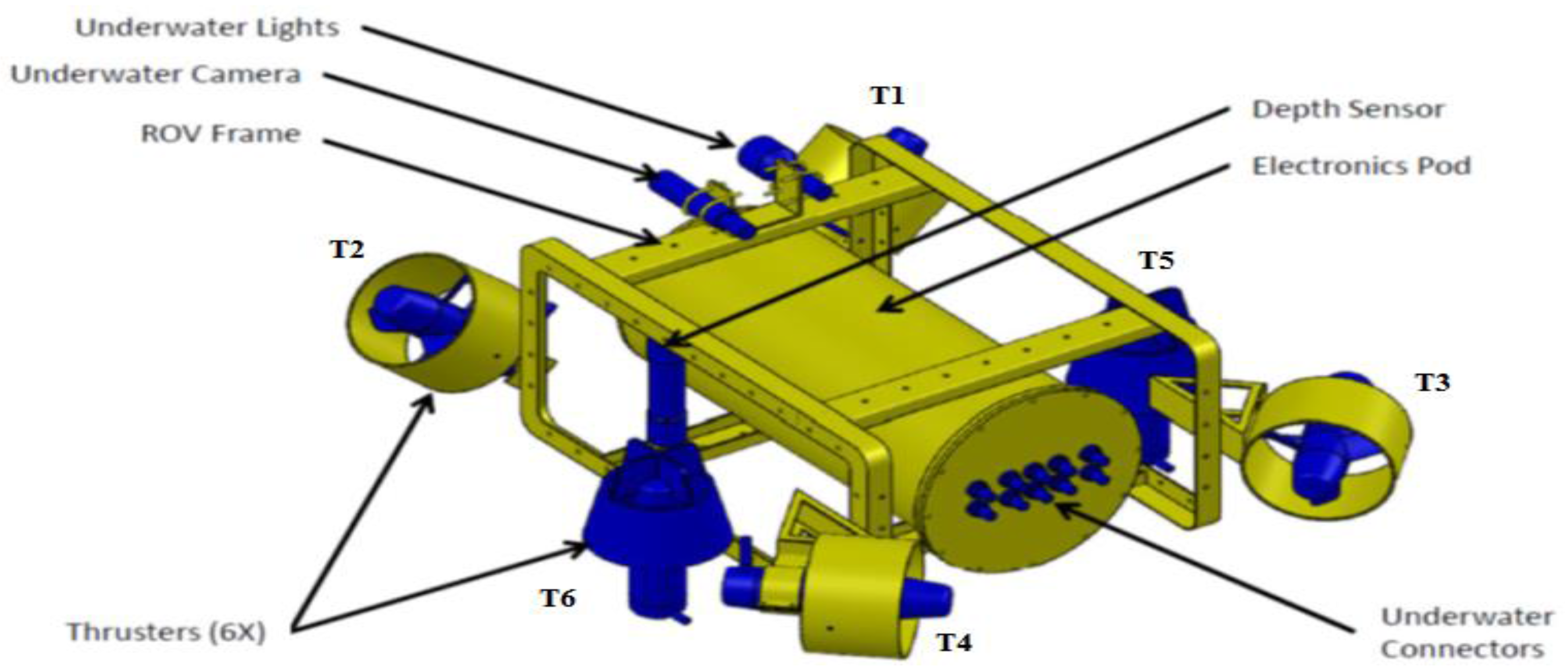
The position of the thruster on the ROV (as seen in Figure 1) is defined by the thrusters’ configuration matrix, T. As mentioned in the nonlinear ROV dynamic equation, the left hand-side of the equations refers to the input forces and moments to the ROV model. These input forces and moments are determined based on the summation of the force and moment equations in the six DOFs. The force and moments for the open-hoop configuration are as follows.

$$\begin{array}{c}\left[\begin{array}{c}{\tau }_x\\ {\tau }_y\\ {\tau }_z\\ {\tau }_{\varphi }\\ {\tau }_{\theta }\\ {\tau }_{\psi }\end{array}\right]=\stackrel{T}{\overbrace{\left[\begin{array}{cccccc}0& 0& \cos \alpha & \cos \alpha & 0& 0\\ -\cos \beta & \cos \beta & \sin \alpha & -\sin \alpha & 0& 0\\ \cos \beta & \cos \beta & 0& 0& 1& 1\\ \text{0.155cos}\beta & -\text{0.155}\cos \beta & 0& 0& -0.275& \text{0.275}\\ \text{0.3945cos}\beta & \text{0.3945cos}\beta & \text{0.4305cos}\beta & \text{0.4305cos}\beta & \text{-0.0355}& \text{-0.0355}\\ \text{-0.3945sin}\beta & \text{0.3945}\sin \beta & -\text{ 0.6605sin}\beta & \text{0.6605sin}\beta & 0& 0\end{array}\right]}}\stackrel{u}{\overbrace{\left[\begin{array}{c}{\text{u}}_{\text{1}}\\ {\text{u}}_{\text{2}}\\ {\text{u}}_{\text{3}}\\ {\text{u}}_{\text{4}}\\ {\text{u}}_{\text{5}}\\ {\text{u}}_{\text{6}}\end{array}\right]}}\\ \tau =Tu\hfill \end{array}$$

(6)

where ${\text{u}}_{\text{min}}\le {\text{u}}_i\le {\text{u}}_{\text{max}},i=1\dots 6$ are the minimum and maximum thrust output by each thruster and $\tau ={[{\tau }_x{\tau }_y{\tau }_z{\tau }_{\varphi }{\tau }_{\theta }{\tau }_{\psi }]}^{\text{T}}$ is the force and moment vector generated. Here α (=45°) is the orientation angle for T3 and T4 while β (=45°) is the orientation angle for T1 and T2. Similar equations can be established for the closed-hoop configuration.

Figure 1. Six thruster locations on AUVDH platform [27].

Figure 1. Six thruster locations on AUVDH platform [27].

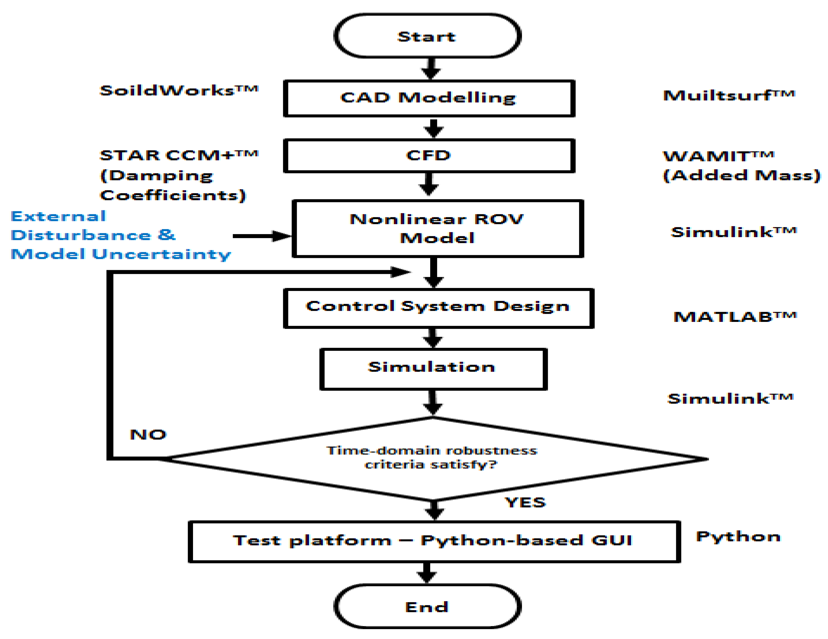
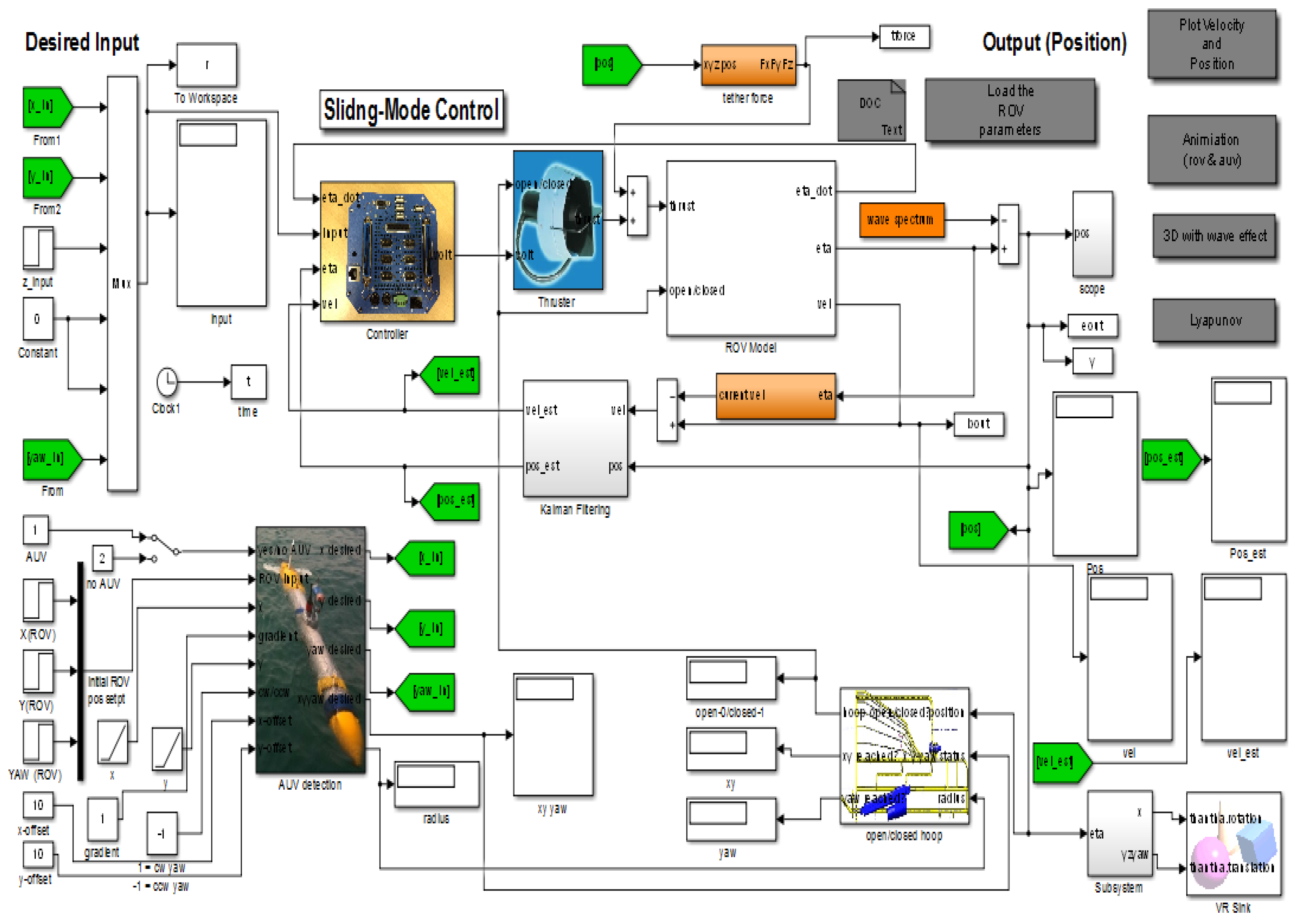
In the proposed hydrodynamics modelling approach, Figure 2 shows the overall approach from numerical modelling to control system design. The computer-aided model of a ROV created using SolidWorks™ and MultiSurf™ is used by computational fluid dynamic (CFD) software such as STAR-CCM+™ and WAMIT™, respectively. As a result, hydrodynamic parameters such as damping and added mass coefficients will be determined for the nonlinear ROV model. For more realistic modelling, the model will be subjected to its inherent model uncertainty due to the numerical computational error and external disturbances. To overcome the model and external disturbance uncertainty, a proposed control system design using sliding-mode based design is applied. The termination of the simulation will depend on satisfying the time-domain criteria and the number of iterations.

Figure 2. Overall flow chart of AUVDH modelling to control system design.

Figure 2. Overall flow chart of AUVDH modelling to control system design.

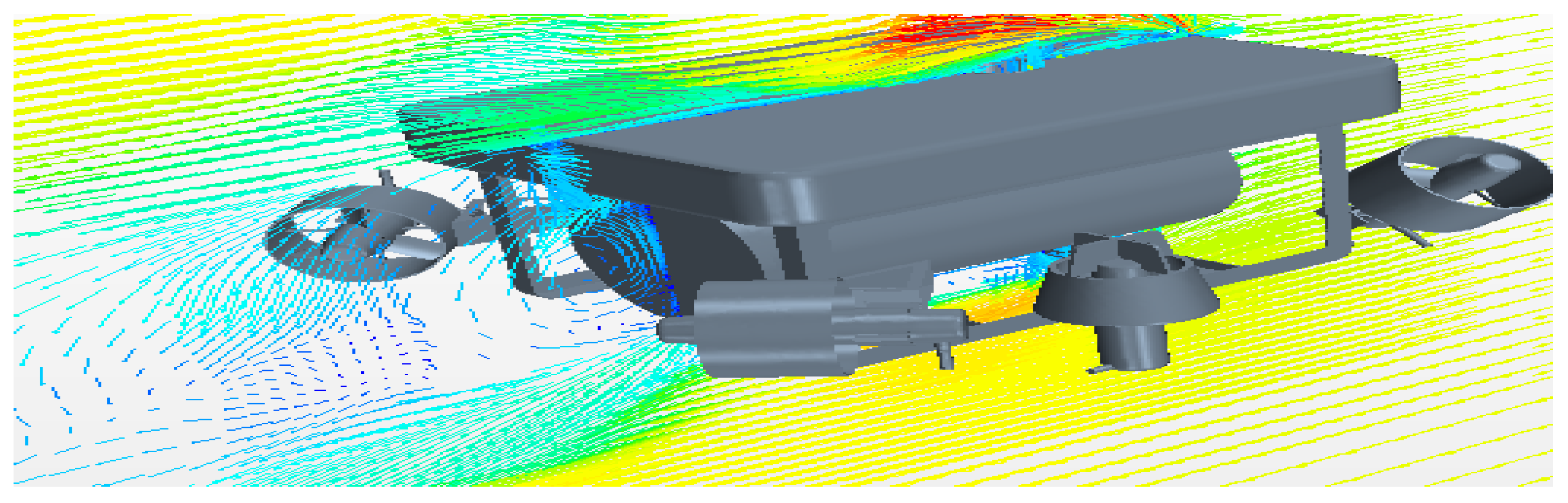
Figure 3 shows the geometrical model of the ROV. The major components of the ROV such as floater, pod, frame and thrusters, are modelled to ensure the flow characteristic is similar to the actual design. As Figure 3 depicted, the ROV is actuated by six thrusters in six DOFs (namely: surge, sway, heave, roll, pitch, and yaw). The docking hoop for docking the AUV is not included in the model. The rigid-body mass and inertia properties with respect to the centre of gravity of the ROV, are determined using the CAD software. The vehicle has a weight of 135 kg, volume of 0.05 m³, and surface area of 4.75 m². Hence, the rigid-body ROV mass inertia can be written as:

$$M_{RB}=\left[\begin{array}{cccccc}135.00& 0& 0& 0& 0& 0\\ 0& 135.00& 0& 0& 0& 0\\ 0& 0& 135.00& 0& 0& 0\\ 0& 0& 0& 2.51& 0& 0\\ 0& 0& 0& 0& 3.38& -0.01\\ 0& 0& 0& 0& -0.01& 1.73\end{array}\right]$$

(7)

The overall damping effect of ROV is described as a sum of linear damping, drag and the vortex shedding (nonlinear damping). The ROV is designed to be self-stabilizable in pitch and roll motion. The viscous effect of the flow causes the non-linear force and moment under a small pitch angle condition to be negligible. The linear coefficients are adequate to represent the force and moments due to the inviscid part of the flow when ROV is operating at a slow speed (less than 2 m/s) [1] and small pitching angle.

Figure 3. Vector plot at centre plane of AUVDH at 0.5 m/s [26].

Figure 3. Vector plot at centre plane of AUVDH at 0.5 m/s [26].

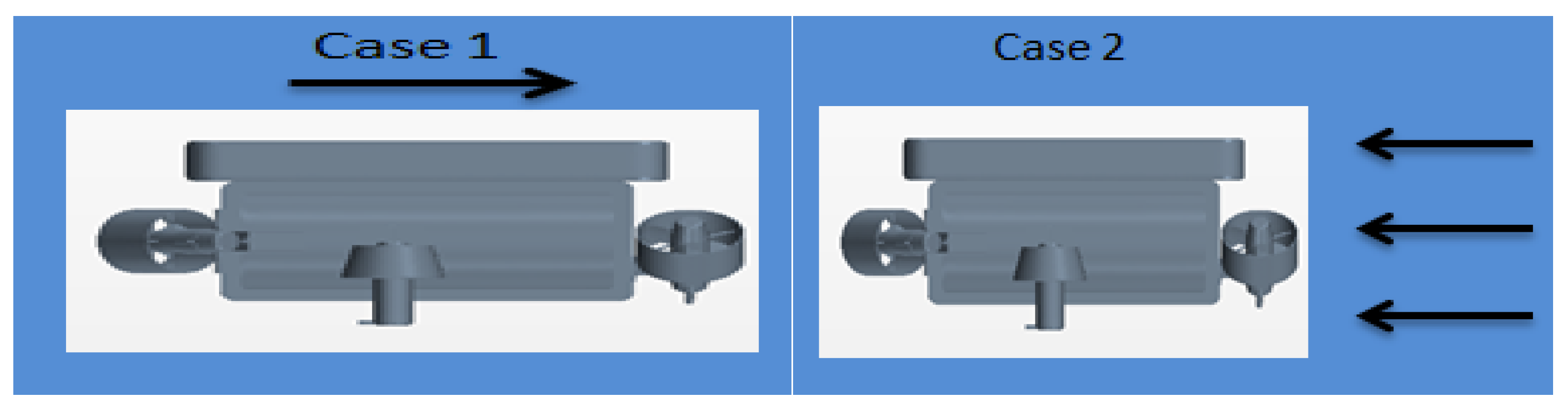
Thus, the ROV hydrodynamic damping matrix D is simplified due to ROV working at a speed approximately equal to 0.5 m/s (angular speed of 0.3 rad/s). The off-diagonal elements in the damping matrix D(v) are small compared to those diagonal elements on the underwater vehicle. Therefore, this hydrodynamic damping matrix becomes: $\text{diag}\left[\left\{X_u,Y_v,Z_w,K_p,M_q,N_r\right\}\right]$ . As shown in Figure 4, Case 1 shows the real situation where the ROV moves forward at a certain speed in a static fluid domain. However in CFD simulation, the ROV was made static and the flow is at opposite direction (Case 2) due to the drag force depends only on the relative motion between the fluid and the vehicle. Hence, it helps to simplify the modelling of the ROV boundary conditions and meshing.

Figure 4. Flow on CFD models for AUVDH [26].

Figure 4. Flow on CFD models for AUVDH [26].

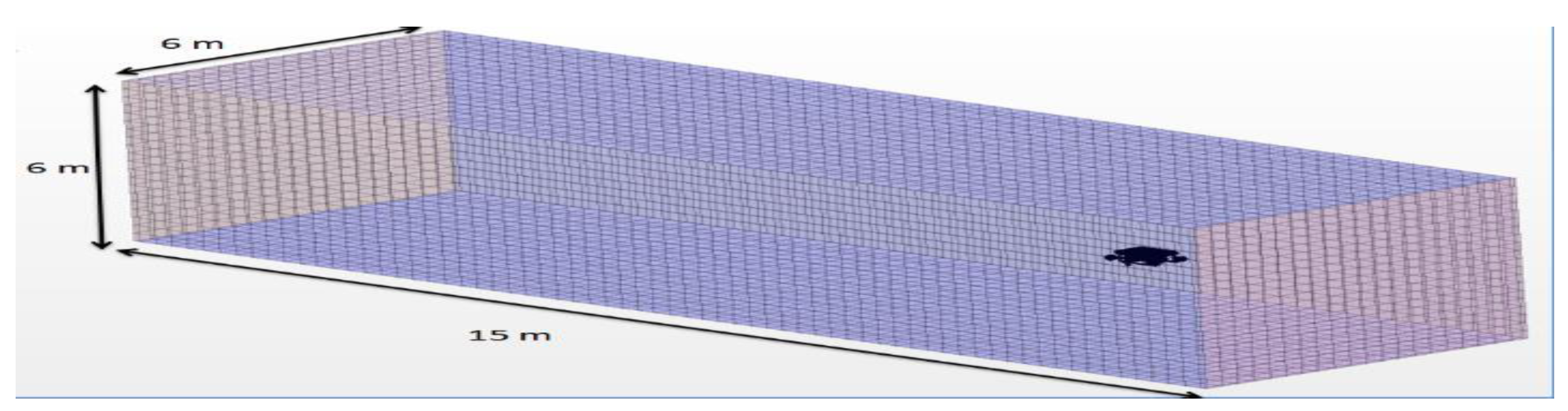
A turbulence model with unsteady three-dimensional flow was built for the Reynolds number flow condition greater than 1.0 × 10⁶. The Shear-Stress-Transport (SST) model was used in CFD software STAR CCM+. The flow in fluid domain is expected to be turbulent and isothermal. The fluid properties of water remain unchanged throughout the simulation process. The temperature is fixed at 20 degree Celsius and the water is modelled as an incompressible fluid. It is impractical to set the fluid domain to be infinitely large to analyse damping force acting on ROV in CFD or in towed tank tests. The suggest dimension is around 10 to 20 times larger than the dimension of the ROV (see Figure 5) to ensure the accuracy [11] of the actual flow domain around the ROV.

Figure 5. Meshing for flow domain around AUVDH [26].

Figure 5. Meshing for flow domain around AUVDH [26].

Table 1 shows the drag coefficient of ROV in the three principle motions. The flow in domain was simulated at different speeds using STAR CCM+. It also shows the drag moment versus angular velocity in yaw direction.

With that, the linear and quadratic hydrodynamic damping matrix for ROV is written as:

$$D_L=-\text{diag}\{[\begin{array}{cccccc}3.221& 3.291& 5.682& 0.& 0& 0\end{array}]\}$$

(8a)

$$D_Q=-\text{diag}\{[\begin{array}{cccccc}105.300& 139.600& 273.800& 0& 0& 6.079\end{array}]\}$$

(8b)

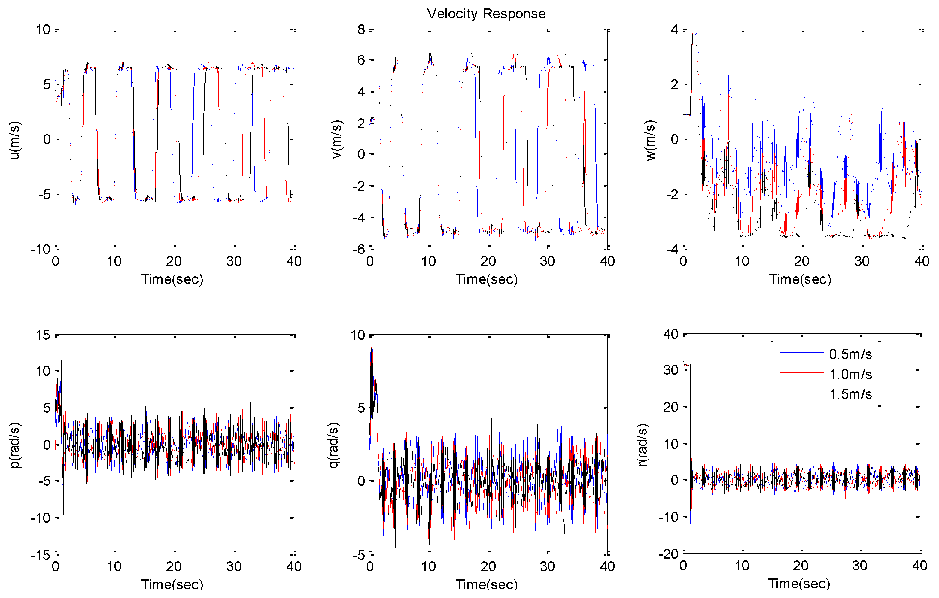
In summary, the results show that surge motion has the lowest damping while the heave motion has the largest drag force. The values of linear damping coefficients are less than the quadratic terms due to its velocity square term. This may be due to the interaction of the thrusters that was not included in the CFD model.

The hydrodynamic added coefficients of the AUVDH are analysed and presented. The added mass and inertia are independent of the wave circular frequency for a fully submerged vehicle. The added mass coefficients matrix for a ROV can be written as follow:

$$M_A=\left[\begin{array}{cccccc}{X}_{\dot{u}}& X_{\dot{v}}& X_{\dot{w}}& X_{\dot{p}}& X_{\dot{q}}& X_{\dot{r}}\\ Y_{\dot{u}}& Y_{\dot{v}}& Y_{\dot{w}}& Y_{\dot{p}}& Y_{\dot{q}}& Y_{\dot{r}}\\ Z_{\dot{u}}& Z_{\dot{v}}& Z_{\dot{w}}& Z_{\dot{p}}& Z_{\dot{q}}& Z_{\dot{r}}\\ K_{\dot{u}}& K_{\dot{v}}& K_{\dot{w}}& K_{\dot{p}}& K_{\dot{q}}& K_{\dot{r}}\\ M_{\dot{u}}& M_{\dot{v}}& M_{\dot{w}}& M_{\dot{p}}& M_{\dot{q}}& M_{\dot{r}}\\ N_{\dot{u}}& N_{\dot{v}}& N_{\dot{w}}& N_{\dot{p}}& N_{\dot{q}}& N_{\dot{r}}\end{array}\right]$$

(9)

where $X_{\dot{u}}$ is the added mass along X-axis due to an acceleration $\dot{u}$ in X-direction, $X_{\dot{v}}$ is the added mass along X-axis due to an acceleration $\dot{v}$ in Y-direction, and so forth.

On the other hand, the corresponding added Coriolis and centripetal matrix is represented.

$$C_A(v)=\left[\begin{array}{cccccc}0& 0& 0& 0& -a_3& a_2\\ 0& 0& 0& a_3& 0& -a_1\\ 0& 0& 0& -a_2& a_1& 0\\ 0& -a_3& a_2& 0& -b_3& b_2\\ a_3& 0& -a_1& b_3& 0& -b_1\\ -a_2& a_1& 0& -b_2& b_1& 0\end{array}\right]$$

(10)

where

$$\begin{array}{l}{a}_1=X_{\dot{u}}u+X_{\dot{v}}v+X_{\dot{w}}w+X_{\dot{p}}p+X_{\dot{q}}q+X_{\dot{r}}r\\ a_2=X_{\dot{v}}u+Y_{\dot{v}}v+Y_{\dot{w}}w+Y_{\dot{p}}p+Y_{\dot{q}}q+Y_{\dot{r}}r\\ a_3=X_{\dot{w}}u+Y_{\dot{w}}v+Z_{\dot{w}}w+Z_{\dot{p}}p+Z_{\dot{q}}q+Z_{\dot{r}}r\\ b_1=X_{\dot{p}}u+Y_{\dot{p}}v+Z_{\dot{p}}w+K_{\dot{p}}p+K_{\dot{q}}q+K_{\dot{r}}r\\ b_2=X_{\dot{q}}u+Y_{\dot{q}}v+Z_{\dot{q}}w+K_{\dot{q}}p+M_{\dot{q}}q+M_{\dot{r}}r\\ b_3=X_{\dot{r}}u+Y_{\dot{r}}v+Z_{\dot{r}}w+K_{\dot{r}}p+M_{\dot{r}}q+N_{\dot{r}}r\end{array}$$

(11)

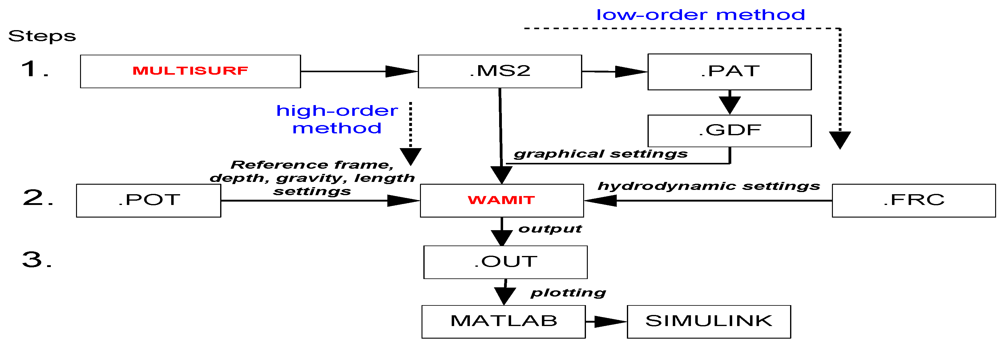
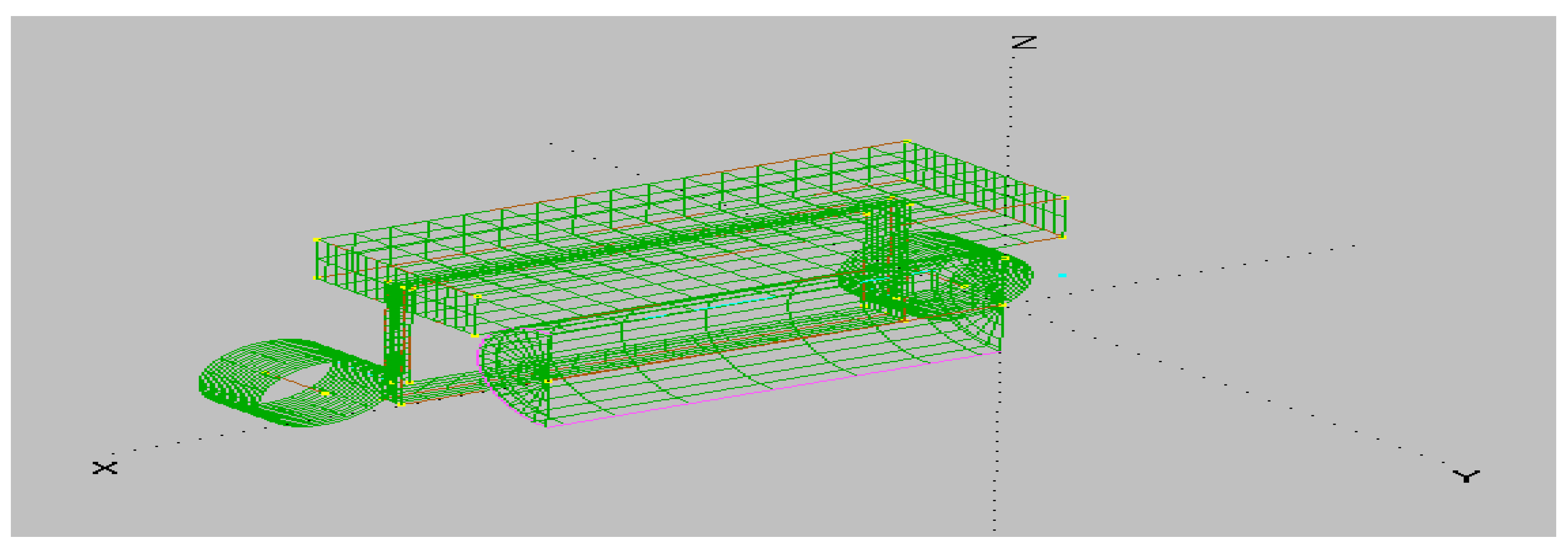
The surface-based computer aided design (CAD) software MultiSurf™ is used to model the geometry of the AUVDH. According to the WAMIT™ manual [28], MultiSurf™ was designed to operate with WAMIT™. It is able to export the necessary file for WAMIT™ applications. The panel surfaces of the AUVDH geometry is shown in Figure 6. As observed, only half of the ROV is modelled due to the symmetry of the vehicle in XZ-plane. This greatly reduces the complexity of the added mass matrix and computation time required by WAMIT™. Since the AUVDH consists of multi-component, these components were drawn simultaneously in MultiSurf™. The mesh of the AUVDH were created using MultiSurf™ and WAMIT™ to compute the added mass matrix.

Figure 6. Finite surface panels generation using MultiSurf™ on AUVDH [26].

Figure 6. Finite surface panels generation using MultiSurf™ on AUVDH [26].

The geometry file created by MultiSurf™ was imported to WAMIT™. The low-order panel method was used. The output file created using WAMIT™ can be imported into MATLAB™ for analysis. Figure 7 illustrates the procedure of using MATLAB™ to analyse the hydrodynamic added mass.

Figure 7. Program flowchart to determine added mass coefficients for AUVDH [26].

Figure 7. Program flowchart to determine added mass coefficients for AUVDH [26].

Before using the WAMIT™ to test the AUVDH, a study of the empirical results of a 2-m diameter sphere to verify the program setup and parameters was used. The theoretical added mass of a sphere is $A=2/3\pi \rho r^3$ for the three translational motions; surge, sway, and heave. The added mass of the sphere can be written as $A=2/3\pi r^3$ through normalizing the mass against density. Table 2 shows the low-order method results of the sphere.

Table 2. Low-order method for sphere [26].

Panel Number	Numerical Results			Theoretical Results
	Surge	Sway	Heave	Surge	Sway	Heave
256	2.085167	2.085168	2.073719	2.0944	2.0944	2.0944
512	2.084073	2.084074	2.087820
1024	2.083766	2.083768	2.091414
Errors				−0.5%	−0.5%	−0.1%

Table 2. Low-order method for sphere [26].

Panel Number	Numerical Results			Theoretical Results
	Surge	Sway	Heave	Surge	Sway	Heave
256	2.085167	2.085168	2.073719	2.0944	2.0944	2.0944
512	2.084073	2.084074	2.087820
1024	2.083766	2.083768	2.091414
Errors				−0.5%	−0.5%	−0.1%

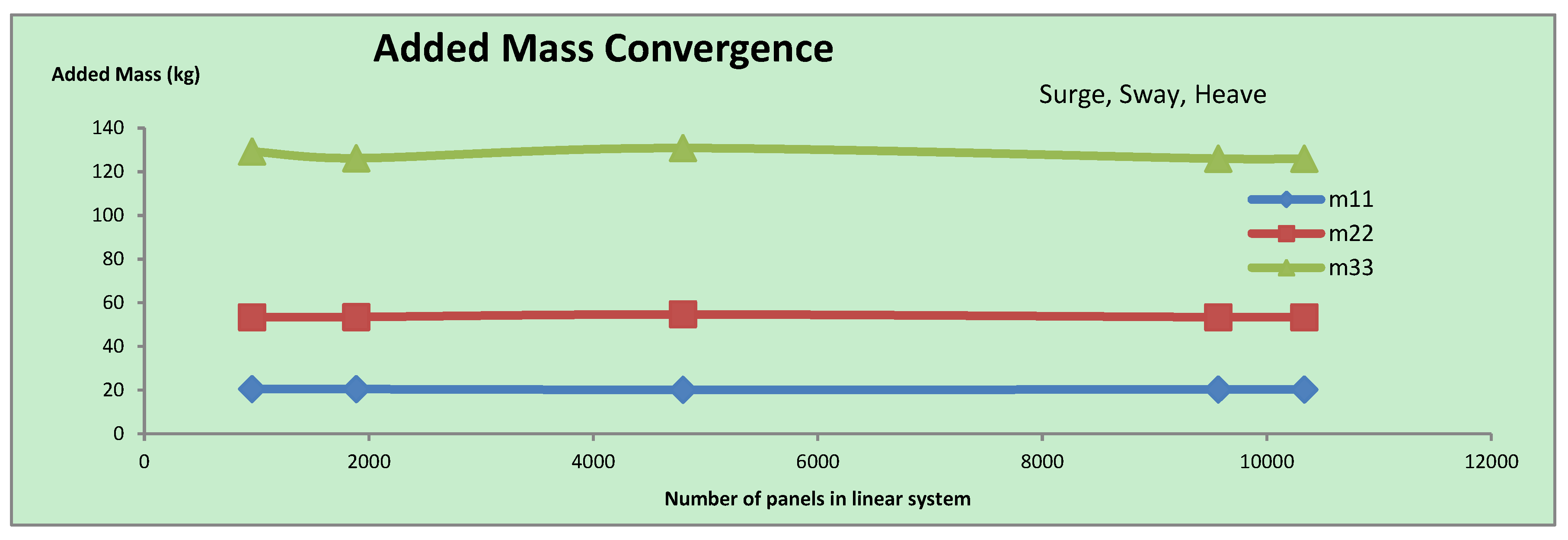
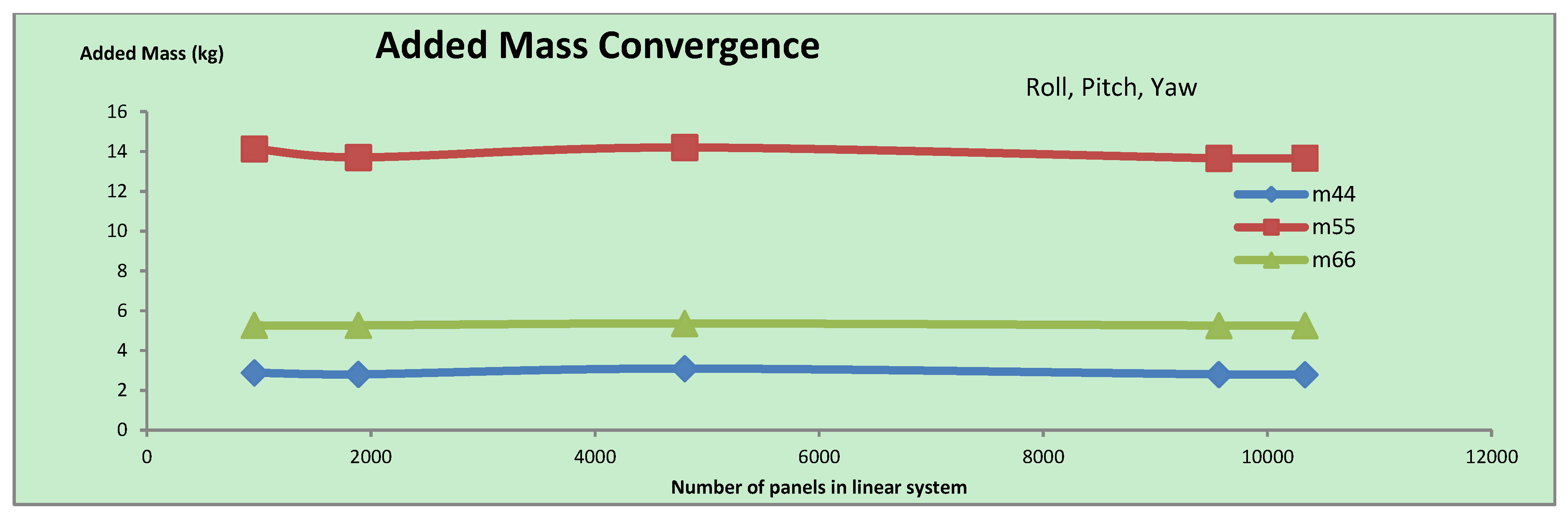
As seen in Table 2, the numerical results obtained from WAMIT™ low-order method have a small difference compared with the theoretical results. The above case study identifies the input parameters settings that are suitable and accurate to compute the added mass coefficient of the AUVDH. The AUVDH was then modelled using MultiSurf™ and imported into the WAMIT™ to solve the problem using the low-order panel method. Only the main components of the AUVDH are drawn to reduce the complexity of the geometry. The convergence tests of the added mass of the AUVDH against various panel numbers are shown in Figure 8 and Figure 9. As observed from the convergence tests, the added mass results achieved desired value of around 3000 to 4000 panels.

Figure 8. Convergence plot for surge, sway, and heave [26].

Figure 8. Convergence plot for surge, sway, and heave [26].

Figure 9. Convergence plot for roll, pitch, and yaw [26].

Figure 9. Convergence plot for roll, pitch, and yaw [26].

The off-diagonal terms in the added mass are smaller as compared to the diagonal components for most of underwater vehicle with approximately three planes of symmetry in the added mass matrix. The off-diagonal components [1] are usually neglected for a slow-speed operating underwater vehicle. The added mass matrix obtained by MATLAB™ can be further simplified.

$$M_A=-\left[\begin{array}{cccccc}20.392& 0& 0& 0& 0& 0\\ 0& 53.435& 0& 0& 0& 0\\ 0& 0& 126.144& 0& 0& 0\\ 0& 0& 0& 2.802& 0& 0\\ 0& 0& 0& 0& 13.703& 0\\ 0& 0& 0& 0& 0& 5.263\end{array}\right]$$

(12)

The added mass matrix $M_{A }$ of the AUVDH must be positive. The following relations are observed from the matrix: $m_{11}<m_{22}<m_{33}$. A smaller added mass in the surge direction, i.e., m₁₁ has been observed. It is due to the AUVDH has the smallest projection area in the surge direction. The corresponding Coriolis and centripetal added mass matrix from Equation (12) can be written as:

$$C_{A }\left(v\right)=\left[\begin{array}{cc}\begin{array}{c}0\\ 0\\ \begin{array}{c}0\\ 0\\ \begin{array}{c}126.144w\\ -53.435v\end{array}\end{array}\end{array}& \begin{array}{cc}\begin{array}{c}0\\ 0\\ \begin{array}{c}0\\ -126.144w\\ \begin{array}{c}0\\ 20.392u\end{array}\end{array}\end{array}& \begin{array}{cc}\begin{array}{c}0\\ 0\\ \begin{array}{c}0\\ 53.435v\\ \begin{array}{c}-20.392u\\ 0\end{array}\end{array}\end{array}& \begin{array}{cc}\begin{array}{c}0\\ 126.144w\\ \begin{array}{c}-53.435v\\ 0\\ \begin{array}{c}5.263r\\ -13.703q\end{array}\end{array}\end{array}& \begin{array}{cc}\begin{array}{c}-126.144w\\ 0\\ \begin{array}{c}20.392u\\ -5.263r\\ \begin{array}{c}0\\ 2.802p\end{array}\end{array}\end{array}& \begin{array}{c}53.435v\\ -20.392u\\ \begin{array}{c}0\\ 13.703q\\ \begin{array}{c}-2.802p\\ 0\end{array}\end{array}\end{array}\end{array}\end{array}\end{array}\end{array}\end{array}\right]$$

(13)

In summary, the added mass coefficients of the AUVDH were computed by WAMIT™ using both potential flow and panel method theory. The added mass in surge motion is around 20 kg; in sway motion is 53 kg; in heave motion is 126 kg. As shown in Figure 8 and Figure 9, different added mass results with the various numbers of panels are presented were compared. The added mass results tend to converge near to 10,000 panels. By observing the numerical results based on the surface area and shape of the AUVDH, it shows a good relationship with the respectively hydrodynamic parameters. Hence, the AUVDH model is adequate for subsequent control system design.

$$\begin{array}{c}{M}_A=-\text{diag}\{[\begin{array}{cccccc}20.392& 53.435& 126.144& 2.802& 13.703& 5.263\end{array}]\}\\ M_{RB}=\left[\begin{array}{cccccc}135.00& 0& 0& 0& 0& 0\\ 0& 135.00& 0& 0& 0& 0\\ 0& 0& 135.00& 0& 0& 0\\ 0& 0& 0& 2.51& 0& 0\\ 0& 0& 0& 0& 3.38& -0.01\\ 0& 0& 0& 0& -0.01& 1.73\end{array}\right]\\ D_L=-\text{diag}\{[\begin{array}{cccccc}3.221& 3.291& 5.682& 0.679& 5.319& 1.275\end{array}]\}\\ D_Q=-\text{diag}\{[\begin{array}{cccccc}105.300& 139.600& 273.800& 15.520& 33.240& 0.204\end{array}]\}\end{array}$$

(14)

3. AUVDH Simulation Platform

The AUVDH dynamics include the inertia mass and added mass model, Coriolis and centripetal forces, Euler’s transformation, gravitational and buoyancy forces, damping forces and thruster model. The simulation models for each subsystem are shown in this section.

3.1. AUVDH Simulation Model

The overall view of the AUVDH dynamic model [27] can be seen in Figure 10. The desired input to the AUVDH is on the left-hand side of the block diagrams that is a joystick input to move the AUVDH manually. The error signal can be computed by finding the difference between the desired inputs and actual feedback of the AUVDH. The input signal is then passed to the controller to control the AUVDH. The thrust configuration on the AUVDH is set by the thrust configuration matrix. The tether force (in orange colour) is treated as an external disturbance acting against the thrust inputs in X, Y and Z direction. The total forces to the AUVDH body dynamics are contributed by the rigid body and added mass matrix, Coriolis and centripetal forces, damping forces, and gravitational and buoyancy forces. The sum of all these forces is then multiplied by the inverse of the rigid body and added mass matrix to obtain the acceleration of the vehicle. With the integration function, the velocities are computed for the next iteration until end of the simulation time. In addition to obtaining the body-fixed velocities, the Earth-fixed position can be found by the Euler’s transformation block. The Euler’s angle is used to calculate the gravitational and buoyancy forces. The external environmental forces (in orange colour) due to the wave and sea current are acting on the AUVDH.

Figure 10. AUVDH Model using Simulink™.

Figure 10. AUVDH Model using Simulink™.

The dynamics of the thruster (namely: Tecnadyne Model 520 and 540) are obtained from the 2D lookup tables. To determine the thrust inputs to the six thrusters, an inverse operation on T is performed. Note that the multi-ports switches are used to trigger the hoop to open or close.

3.2. Tether Model

A tether of length 50 m is fastened in the zero start coordinate The tether weight is approximately, 1.1 N/m, diameter is 0.0177 m and the Young’s Modulus is 0.025 GPa for polyurethane elastomer. We solve the 3D Catenary Boundary Value Problem (BVP) using the MATLAB™ routine [25]. An estimate of the end force given the end point distance or the AUVDH final Earth-fixed position can be computed. For example, the MATLAB^TM command line: sol = cable3dbvp ([10 10 50], 50). The calculated end force in X, Y, and Z directions becomes [46.43 46.49 257.67] N, respectively. This routine will be used to calculate the force exerted on the AUVDH simulation model while manoeuvring in water. However, it is quite computationally-consuming to compute the tether forces for every change in the end point coordinates. Instead, a backpropagation neural network is used to model the tether forces.

A neural network models the tether dynamics force at the end point of the AUVDH. The training function used is Levenberg-Marquardt (trainlm) and the performance mean square error (MSE) using MATLAB™ toolbox is used. A total of 10 neurons and one hidden layer are used. The inputs are the X, Y, and Z end point of the tether. While the outputs are the respective force on the body-fixed coordinate of the AUVDH at its CG. As shown in Figure 11, the neural network model (difference in the target and the output) has largely an absolute error of 3.594, and they are also closely correlated in Figure 11. Thus, the neural network model gives a close result to the actual computed values from 3D Catenary BVP.

Figure 11. Results of backpropagation neural network model for tether model for training, validation and test (a) error histogram plot (b) regression plot where R values measure correlation between outputs and targets (R value of 1 means a close relationship, and 0 means a random relationship).

Figure 11. Results of backpropagation neural network model for tether model for training, validation and test (a) error histogram plot (b) regression plot where R values measure correlation between outputs and targets (R value of 1 means a close relationship, and 0 means a random relationship).

3.3. Launch and Recovery Process Model

The launch and recovery process [27] of the AUV consists of deploying the AUVDH into the water using a simple remote-operated rope winch. The mission is in a standby mode and begins when the AUVDH reaches the mission depth and steers away from the aft of the launch vessel. The AUVDH executes its mission with the aid of external sensors. Data is logged during the mission. After the recovering of the AUV is completed, the AUVDH ascend to the surface near to the winch. The AUVDH is retrieved with the help of the winch with hook. A new mission can be performed and the whole process is repeated.

A robust control system such as sliding-mode controller [27] will be used to control the AUVDH in order to recover of the AUV. The control strategy is to steer the AUVDH away from the aft before submerging, and align the AUVDH to the incoming AUV. The AUVDH starts to close the hoop when the distance between the vehicles reached around 50 m. With a current speed of 1.5 m/s, the time for AUV to reach AUVDH is around 33 s. This will be the time available for the AUVDH to close its hoop for the incoming AUV. However it can be difficult to determine the time as the current speed and direction changes with time. Likely scenario of path misalignment can be seen in Figure 12. As observed, the heading or/and Y-offset in either direction can happen during the path alignment. The control strategy is tasked to detect the presence of the AUV first and try aligning itself to the incoming vehicle. If it fails, the second attempt will be activated as the AUVDH is not designed to chase after the AUV.

Figure 12. AUV detection and recovery scenarios [27]. (a) AUV moving toward AUVDH at different yaw angle (b) AUV moving toward AUVDH at different sway direction(c) AUV moving toward AUVDH at different yaw angle and sway direction.

Figure 12. AUV detection and recovery scenarios [27]. (a) AUV moving toward AUVDH at different yaw angle (b) AUV moving toward AUVDH at different sway direction(c) AUV moving toward AUVDH at different yaw angle and sway direction.

To accomplish the control strategy, the following control architecture is used. As observed, the control system uses the nonlinear AUVDH model determined in the earlier part of the work. The first part of the control is to detect the presence of the AUV using the abovementioned detection method. Path planning (with sufficient time) and speed correction (insufficient time) are required to provide robustness due to the uncertainty in the time allocated for hoop triggering that depends on the current speed. The sliding-mode controller (SMC) [27] controls both the position and velocity of the AUVDH such that the path is maintained (i.e., aligned with the correct heading and path of the incoming AUV). The control signal then triggers the respective thrusters to control the AUVDH to its desired position and speed. The controller is designed to deal with the current and model uncertainty in a theoretic manner as shown below.

The Lyapunov function candidate can be written as such:

$$V(t)=\frac{1}{2}{s}^{T}Ms$$

(15)

The time derivative yields:

$$\dot{V}(t)=s^{T}M\dot{s}$$

(16)

Here $M\dot{s}=M(\ddot{\mathsf{\eta }}+\lambda \dot{\mathsf{\eta }})$ since ${\ddot{\mathsf{\eta }}}_d=0,{\dot{\mathsf{\eta }}}_d=0$ and $\ddot{\mathsf{\eta }}=J(\mathsf{\eta })\dot{v}+\dot{J}(\mathsf{\eta })v$, it can be written as:

$$\begin{array}{ll}\dot{V}(t)& =s^{T}M[J(\mathsf{\eta })\dot{v}+\dot{J}(\mathsf{\eta })v+\lambda \dot{\mathsf{\eta }}]\\ & =s^{T}M\{J(\mathsf{\eta })M^{-1}[-C_o(v)v-D(v)\\ & -g(\mathsf{\eta })+\Delta (v,\mathsf{\eta },v_c,{\dot{v}}_c)\text{]}\\ & +s^{T}M[J(\mathsf{\eta })M^{-1}Tu+\dot{J}(\mathsf{\eta })v+\lambda \dot{\mathsf{\eta }}]\}\end{array}$$

(17)

where the current velocity is included as relative velocity.

$$v_r=v-v_c$$

(18)

Here $v_c={[\begin{array}{cccccc}{u}_c& v_c& w_c& 0& 0& 0\end{array}]}^{\text{T}}$ is the current velocity vector in body fixed frame, and $\Delta (v,\mathsf{\eta },v_c,{\dot{v}}_c)$ is the lumped uncertainty defined as:

$$\Delta M\dot{v}+\Delta C(v)v+\Delta g(\mathsf{\eta })+\Delta D(v_r)$$

(19)

Thus, the control law can be defined as:

$$\begin{array}{l}u=T^{+}[C_o(v)v+D(v)+g_o(\mathsf{\eta })\\ -\Delta (v,\mathsf{\eta },v_c,{\dot{v}}_c)\stackrel{\text{SMC controller}}{\overbrace{-K_{sp}\mathrm{sgn}(s)-K_{si}s-K_{sd}v}}]\end{array}$$

(20)

where $K_{sp},K_{si},K_{sd}$ are the controller gains and $T^{+}={(T^{T}T)}^{-1}{T}^T$ is the Moore–Penrose pseudo-inverse.

Substituting the control law into $\dot{V}$ yields:

$$\begin{array}{l}\dot{V}(t)=s^{T}M[-K_{sp}\mathrm{sgn}(s)-K_{si}s-K_{sd}v\\ +\Delta (v,\mathsf{\eta },v_c,{\dot{v}}_c)+\dot{J}(\mathsf{\eta })v+\lambda \dot{\mathsf{\eta }}]\end{array}$$

(21)

Choose $K_{sp},K_{si},K_{sd}$ large enough so that $K_{si}{I}_6$$\ge \dot{J}(\mathsf{\eta })+\lambda J(\mathsf{\eta })$$+\Delta (v,\mathsf{\eta },v_c,{\dot{v}}_c)$, and $\lambda$ is small such that $\dot{V}(s(t))\le 0$. Notice that $\left|\dot{J}(\mathsf{\eta })\right|$ and $\left|J(\mathsf{\eta })\right|$ do not exceed one. The bounds of the lumped uncertainty are assumed to be given as: $\Delta (v,\mathsf{\eta },v_c,{\dot{v}}_c)\le \rho$, and $v(t)$ is small, $\dot{V}\le 0\Rightarrow V(t)\le 0\Rightarrow$$s$ is bounded. This implies that $\ddot{V}$ must be uniformly continuous. Application of Barbalat’s lemma shows that $s\to 0$ and thus $\tilde{\mathsf{\eta }}\to 0$ as $t\to \infty$.

This technique can yield good tracking with the price of excessive discontinuous switching across $s=0$ or chattering. In addition, a boundary layer around the sliding surface with thickness $\Phi \in {\Re }^6(\Phi (.)>0)$ is adopted to avoid chattering. The vehicle dynamics remains “inside” this boundary layer with no switching. If the region outside the layer is reached, then switching is carried out. Mathematically, it can be expressed as:

$$sat(s/\Phi )=\{\begin{array}{ccc}\mathrm{sgn}(s/\Phi ),& for& \left|s/\Phi \right|\ge 1\\ s/\Phi & for& \left|s/\Phi \right|<1\end{array}$$

(22)

Including the boundary layer in preceding equation, the control becomes:

$$\begin{array}{l}u=T^{+}[C(v)v+D(v)+g(\mathsf{\eta })\\ -\Delta (v,\mathsf{\eta },v_c,{\dot{v}}_c)-K_{sp}sat(s/\Phi )-K_{si}s-K_{sd}v]\end{array}$$

(23)

The Simulink™ block diagram for the sliding-mode controller consists of a subsystem to compute the sliding surface and to compensate for the nonlinear function. The controller has the following parameters: bandwidth = 111; boundary layer thickness = 4 and other controller gains: $k_s=20;k_{sv}=1\times {10}^{-4};k_{sd}=55$ as shown in the last three terms of Equation (23). We assume the controller gains are similar for each DoF. However, they can be adjusted to tune the AUVDH performance.

The sliding-mode control works as follows: the tracking error is negative (positive), indicating that the position is too small, the control input will be increased (or decreased) in order to increase the output. The “energy” of the system diminishes slowly as it reaches the sliding surface (near to zero tracking error). In this simulation, the AUVDH was commanded to move in vertical plane followed by horizontal plane, that is $z_d=5m,{\psi }_d={45}^{\text{o}}$. By simulating the sliding-mode controller, the position and velocity time responses can be seen in Figure 13a and Figure 14. The 2D animation of AUVDH was done offline after the simulation was completed. It basically consists of many frames of AUVDH motions which are combined to form an animation of the AUVDH from the start to the final AUV recovery as seen in Figure 13b.

As observed in Figure 14, the position response yields good tracking without excessive discontinuous switching or chattering, as seen in the velocity plots. With the use of the boundary layer around the sliding surface, the chattering has disappeared and results in less oscillatory responses in the velocity. In Figure 13a and Figure 14, the roll and pitch DOF are stable without any control. Further improvement can be performed by tuning the sliding-mode controller gains.

Figure 13. Position response for $z_d=5m,{\psi }_d={45}^{\text{o}}$ (a) position of AUVDH during entire recovery operation (b) top view of AUV and AUVDH during final recovery.

Figure 13. Position response for $z_d=5m,{\psi }_d={45}^{\text{o}}$ (a) position of AUVDH during entire recovery operation (b) top view of AUV and AUVDH during final recovery.

Figure 14. Velocity response for $z_d=5m,{\psi }_d={45}^{\text{o}}$.

Figure 14. Velocity response for $z_d=5m,{\psi }_d={45}^{\text{o}}$.

The impact of the sea current acting on the AUVDH during manoeuvring was studied. Further tuning on the sliding-mode control was performed at different current speed. As observed in Figure 15 and Figure 16, the desired position ($y_d=3\text{m, }{z}_d=5m,{\psi }_d={45}^{\text{o}}$) is affected when the sea currents exceed 1 m/s. The roll and pitch motions remain unperturbed and small. The velocity responses increase due to the current but they are regulated around the zero value. The AUVDH distance travelled is around x = 10 m, y = 15 m (see Figure 15). The reason for these large distances travelled is due to the current velocity (simulated at 0.5 m/s, 1 m/s and 1.5 m/s). For example, 20–30 s (at current speed of 1 m/s), the AUVDH moves to around 20–30 m. The robust design simulation of autonomous underwater vehicle docking hoop during recovery operation after a search and rescue mission was successfully simulated and shown to work under the external wave, current, and tether force.

As seen in next section, a real-time display on the surface with joystick control involving man-in-the-loop will be included into the control system to provide certain robustness in the event of fault and other unforeseen conditions.

Figure 15. Sea current disturbance on AUVDH position ($y_d=3\text{m, }{z}_d=5m,{\psi }_d={45}^{\text{o}}$).

Figure 15. Sea current disturbance on AUVDH position ($y_d=3\text{m, }{z}_d=5m,{\psi }_d={45}^{\text{o}}$).

Figure 16. Sea current disturbance on AUVDH velocity ($y_d=3\text{m, }{z}_d=5m,{\psi }_d={45}^{\text{o}}$).

Figure 16. Sea current disturbance on AUVDH velocity ($y_d=3\text{m, }{z}_d=5m,{\psi }_d={45}^{\text{o}}$).

4. AUVDH GUI Test Platform

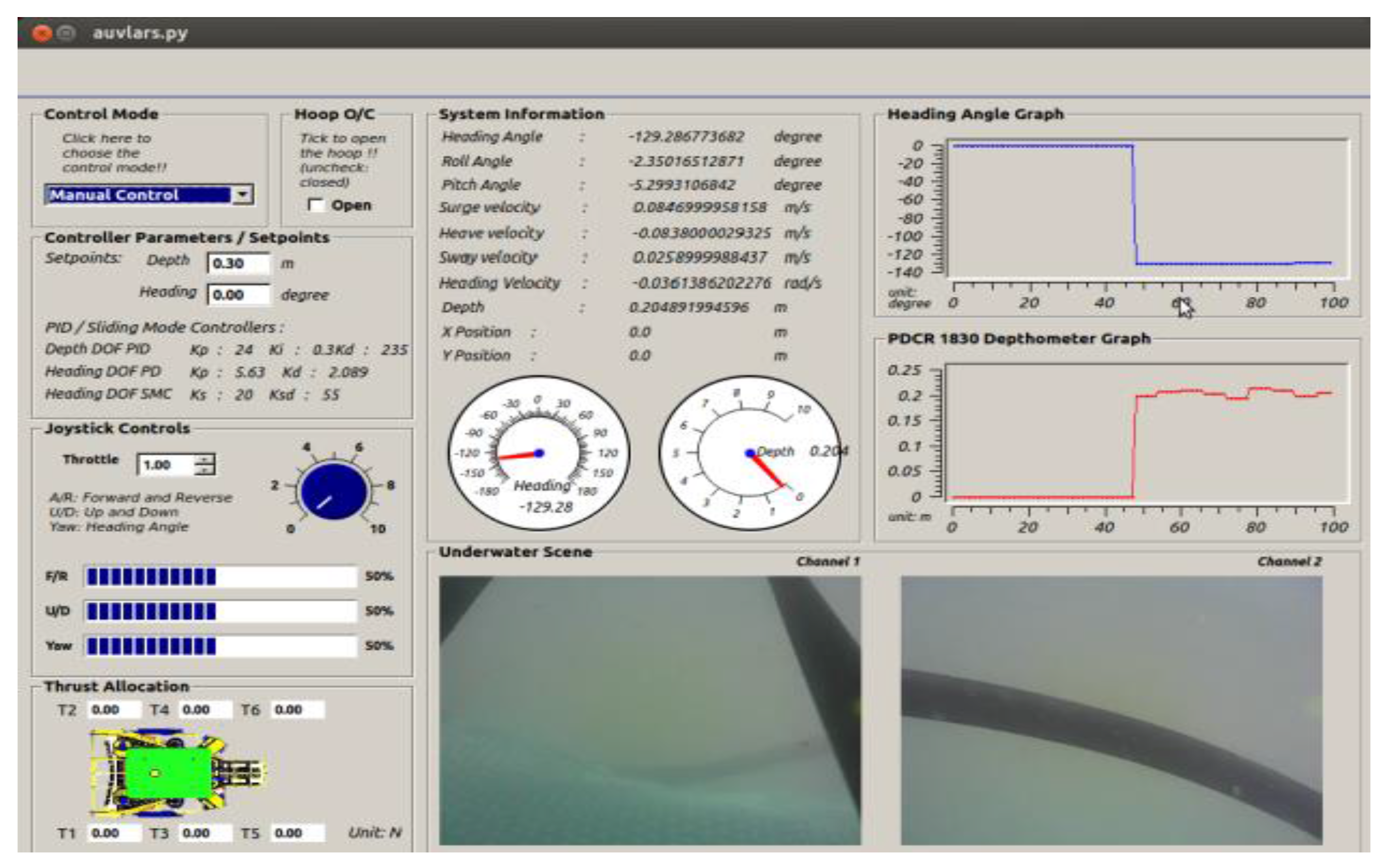
A graphical user interface (GUI) is seen as an essential requirement for enhanced operator dexterity. Tele-presence systems have been investigated as a means of realizing highly dexterous and intuitive systems for AUVDH. The AUVDH GUI control system panel consists of two primary functions: send control commands to control the thrusters manually and automatically; and display sensors and thrusters’ status in real-time. The actual layout of the GUI control panel is shown in Figure 17.

Figure 17. AUVDH GUI control panel layout.

Figure 17. AUVDH GUI control panel layout.

Creating the AUVDH GUI applications on Linux can be performed in different ways. Using the simplest and the most functional programming languages and libraries under the Linux desktop using the Qt library with the Python programming language, called “PyQt”, was chosen. To facilitate the software development, an integrated development environment (IDE) consisting of a source code editor, build automation tools, and a debugger are needed. Since Python and Qt were chosen, the IDE written in Python, and based on the cross platform Qt GUI toolkit, integrating a flexible editor control is highly desired. Thus, the Eric4Python IDE written in Python and based on the Qt GUI was selected. It includes a plugin system, which allows easy extension of the IDE functionality with plugins downloadable from the Internet. In this project, the GUI control panel was designed using PyQt4, Python 2.7, and the Eric4Python IDE as the integrated development environment.

A brief overall view of the software packages used in the project is described. Qt brings flexibility to embedded development, allowing engineers to create high-performing and modern user-interfaces and applications with built-in productivity-enhancing tools for fast, easy, fully-integrated embedded device application development. The pre-configured embedded development environment, pre-built Qt optimized software stack for immediate deployment to ATHENA III embedded board allows users to get running, and have a working embedded project prototype. The QtGui module contains the graphical components and related classes. These include for example buttons, windows, status bars, toolbars, sliders, bitmaps, colours and fonts. The module enables seamless integration of the Qt GUI library and the OpenGL library. The QtSql module provides classes for working with databases. There are six function modules for the AUVDH GUI. They are namely, control mode, switch control of docking hoop, network connection, thruster readout, and video image display.

5. Results and Discussion

The ROV was tested in a water tank as shown in Figure 18a. A few tests were conducted on the open-loop AUVDH system for sensor fusion and closed loop control. The AUVDH is a tethered and remotely-operated underwater robot as shown in Figure 18b. The AUVDH is powered by a 230VAC power supply. The mass of the vehicle is approximately 135 kg and its dimensions are 1.5 m long × 1 m wide × 1.7 m high. The exterior components consist of a docking hoop to dock the AUV, six thrusters, DVL, altimeter, IMU, floater, and aluminium casing to house the electronics. The heading and position of the AUVDH are actively controlled, and the vehicle is passively stable in both pitch and roll motion. The actuation is provided by six 24VDC brushless electric thrusters. The AUVDH is equipped for position and velocity measurement using DVL, altimeter and IMU.

Figure 18. Experimental test setup of AUVDH (a) near water tank (b) on ground after test.

Figure 18. Experimental test setup of AUVDH (a) near water tank (b) on ground after test.

Few trials in the commanded heave and yaw directions were conducted, as seen in the test images shown in Figure 19. During the experiments, the performance of the open-loop guidance and closed-loop control systems using the sliding-mode controller were fully assessed. Figure 20 and Figure 21 are a small sample of the large amounts of experimental data that were obtained during the tests. Figure 20 show commanded and measured depth and heading, respectively. Figure 21 shows that the roll and pitch angle are self-stabilizable by design. In the results observed, the AUVDH positioning system relied on data provided by IMU and DVL. This creates errors in the calculated position after the double integrations on the acceleration data from the IMU. The dead-reckoning method (the process of calculating one’s current position by using a previously determined position and advancing that position based upon known or estimated speeds over elapsed time) with a Butterworth high-pass filter to remove the bias are used to identify whether the AUVDH moves or remains stationary before performing the integration. The Extended Kalman Filtering (EKF) thread will then be used to estimate the position and velocity of the AUVDH. As shown in the depth measurement, there is a bias of 0.3 m due to the installation of the depth sensor. This was removed to reflect the actual operating depth from the surface. The test results show that the AUVDH is able to perform the station-keeping at a fixed yaw and heave command under the external disturbances.

Figure 19. Experimental test image (yaw then heave) during test in water tank.

Figure 19. Experimental test image (yaw then heave) during test in water tank.

Figure 20. Simulated and measured responses of AUVDH (a) heading response (b) heave response.

Figure 20. Simulated and measured responses of AUVDH (a) heading response (b) heave response.

Figure 21. Simulated and measured response of AUVDH. (a) roll angle response (b) pitch response

Figure 21. Simulated and measured response of AUVDH. (a) roll angle response (b) pitch response

6. Conclusions

This paper has reported a preliminary experimental evaluation of a model-based sliding-mode controller for a low-speed manoeuvring of an actuated remotely-operated vehicle (ROV) named AUV docking hoop (AUVDH). We considered the simple case of an AUVDH plant dynamics model employing constant added mass, buoyancy, linear and quadratic drag, and thrust input. Dynamic modelling and simulation of AUVDH during launch and recovery of the AUV were performed. The tether model was modelled using the backpropagation neural network. The control strategy from launch to recovery in 2D and 3D was simulated using MATLAB™ and Simulink™ prior to actual implementation. The control simulation using a sliding mode controller (SMC) was proposed to control the surge, sway, heave, and yaw positions and velocities of the AUVDH under the sea wave, current and tether forces. In summary, the proposed SMC scheme is able to control the AUVDH during launch and recovery of the AUV under the external disturbances. The experiment tests conducted in water tank shown that the SMC is able to control the depth and yaw position of the AUVDH with small roll and pitch angles. However, the experiments do not demonstrate the effects of variations in controller gains or change due to the thruster configuration matrix and inertia matrix for the closed-hoop condition. The identification and closed-loop comparison with other controllers needs to be performed. We hope to report an experimental evaluation of these conditions on the performance of these controllers in the sea trial.

References

1. Fossen, T.I. Guidance and Control of Ocean Vehicles; John Wiley & Sons Ltd.: Chichester, England, 1994. [Google Scholar]
2. Rauch, C.G.; Purcell, M.J.; Austin, T.; Packard, G.J. Ship of opportunity launch and recovery system for REMUS 600 AUV’s. In Proceedings of the OCEANS 2008, Quebec City, QC, Canada, 15–18 September 2008; pp. 1–4.
3. Kaminski, C.; Crees, T.; Ferguson, J.; Forrest, A.; Williams, J.; Hopkin, D.; Heard, G. 12 days under ice—An historic AUV deployment in the Canadian High Arctic. In Proceedings of the 2010 IEEE/OES Autonomous Underwater Vehicles, Monterey, CA, USA, 1–3 September 2010; pp. 1–11.
4. Hayashi, E.; Kimura, H.; Tam, C.; Ferguson, J.; Laframboise, J.M.; Miller, G.; Kaminski, C.; Johnson, A. Customizing an Autonomous Underwater Vehicle and developing a launch and recovery system. In Proceedings of the 2013 IEEE International Underwater Technology Symposium (UT), Tokyo, Japan, 5–8 March 2013; pp. 1–7.
5. Hagen, P.E.; Storkersen, N.; Marthinsen, B.-E.; Sten, G.; Vestgard, K. Military operations with HUGIN AUVs: Lessons learned and the way ahead. In Proceedings of the OCEAN 2005, Brest, France, 20–23 June 2005; Volume 2, pp. 810–813.
6. Fauske, K.M.; Gustafsson, F.; Hegrenaes, O. Estimation of AUV dynamics for sensor fusion. In Proceedings of the 10th International Conference on Information Fusion, Quebec City, QC, Canada, 9–12 July 2007; pp. 1–6.
7. Sørensen, A.J. Lecture Notes of TMR4240. Marine Cybernetics—Modelling and Control; Department of Marine Technology NTNU: Trondheim, Norway, 2005. [Google Scholar]
8. Johannessen, K.; Meling, T.S.; Haver, S. Joint Distribution for Wind and Waves in the Northern North Sea. IJOPE 2002, 12, 1. [Google Scholar]
9. Blanke, M. Enhanced maritime safety through diagnosis and fault tolerant control. In Proceedings of the IFAC Conference on Control Applications and Marine Systems, CAMS 2001, Glasgow, UK, 18–20 July 2001.
10. Chan, W.L.; Kang, T. Simultaneous Determination of Drag Coefficient and Added Mass. IEEE J. Ocean. Eng. 2011, 36, 422–430. [Google Scholar] [CrossRef]
11. Chin, C.S.; Lau, M.S.W. Modeling and Testing of Hydrodynamic Damping Model for a Complex-Shaped Remotely-Operated Vehicle for Control. J. Mar. Sci. Appl. 2012, 11, 150–163. [Google Scholar] [CrossRef]
12. Eng, Y.; Lau, M.; Chin, C. Added Mass Computation for Control of an Open Frame Remotely-Operated Vehicle: Application using WAMIT and MATLAB. J. Mar. Sci. Technol. 2014, 22, 1–14. [Google Scholar]
13. Ross, A.; Fossen, T.I.; Johansen, T.A. Identification of underwater vehicle hydrodynamic coefficients using free decay tests. In Proceedings of the IFAC Conference on Control Applications in Marine Systems, Ancona, Italy, 7–9 July 2004; pp. 1–6.
14. Morrison, A.T.; Yoerger, D.R. Determination of the hydrodynamic parameters of an underwater vehicle during small scale, nonuniform, 1-dimensional translation. In Proceedings of the Engineering in Harmony with Ocean, OCEANS ’93, Victoria, BC, Canada, 18–21 October 1993; Volume 2, pp. 277–282.
15. Caccia, M.; Indiveri, G.; Veruggio, G. Modeling and identification of open-frame variable configuration unmanned underwater vehicles. IEEE J. Ocean. Eng. 2000, 25, 227–240. [Google Scholar] [CrossRef]
16. Smallwood, D.A.; Whitcomb, L.L. Adaptive identication of dynamically positioned underwater robotic vehicles. IEEE Trans. Control Syst. Technol. 2003, 11, 505–515. [Google Scholar] [CrossRef]
17. Sarkar, T.; Sayer, P.G.; Fraser, S.M. A study of autonomous underwater vehicle hull forms using computational fluid dynamics. Int. J. Numer. Methods Fluids 1997, 25, 1301–1313. [Google Scholar] [CrossRef]
18. Barros, E.A.; Pascoal, A.E.S. Investigation of a method for predicting AUV derivatives. Ocean Eng. 2008, 35, 1627–1636. [Google Scholar] [CrossRef]
19. Chin, CS.; Lum, SH. Rapid modeling and control systems prototyping of a marine robotic vehicle with model uncertainties using xPC Target system. Ocean Engineering. 2011, 38, 2128–2141. [Google Scholar] [CrossRef]
20. Zeng, G.H.; Zhu, J. Study on Key Techniques of Submarine Maneuvering Hydrodynamics Prediction Using Numerical Method. In Proceedings of the Second International Conference on Computer Modeling and Simulation, ICCMS ’10, Hainan, China, 22–24 January 2010; pp. 83–87.
21. Zhang, H.; Xu, Y.R.; Cai, H.P. Using CFD software to calculate hydrodynamic coefficients. J. Mar. Sci. Appl. 2010, 9, 149–155. [Google Scholar] [CrossRef]
22. Tang, S.; Tamaki, U.; Nakatani, T.; Thornton, B.; Jiang, T. Estimation of the hydrodynamic coefficents of the complex-shaped autonomous underwater vehicle TUNA-SAND. J. Mar. Sci. Technol. 2009, 14, 373–386. [Google Scholar] [CrossRef]
23. Chin, C.; Lau, M.W.S.; Low, E. Supervisory Cascaded Controllers Design: Experiment Test on a Remotely-Operated Vehicle. Proc. Inst. Mech. Eng. Part C J. Mech. Eng. Sci. 2011, 225, 584–603. [Google Scholar] [CrossRef]
24. Chin, C.; Lau, M.W.S.; Low, E.; Seet, G. Robust and decoupled cascaded control system of underwater robotic vehicle for stabilization and pipeline tracking. Proc. Inst. Mech. Eng. Part I J. Syst. Control Eng. 2008, 222, 261–278. [Google Scholar] [CrossRef]
25. Sørensen, A.J. Marine Control Systems: Propulsion and Motion Control of Ships and Ocean Structures. Lecture Notes; The Norwegian Institute of Technology, Department of Marine Technology: Trondheim, Norway, 2012; pp. 222–224. [Google Scholar]
26. Lin, J.Y. Computation of Hydrodynamic Damping and Added Mass for a Complex-Shaped Remotely-Operated Vehicle (ROV) for Sufficient Control Purpose. Bachelor’s Thesis, Bachelor of Engineering in Marine Engineering, School of Marine Science and Technology, Newcastle University, Tyne and Wear, UK, May 2014. [Google Scholar]
27. Lin, W.P.; Chin, C.S.; Mesbahi, E. Remote Robust Control and Simulation of Robot for Search and Rescue Mission in Water. In Proceedings of the OCEANS ’14 MTS/IEEE, Taipei, Taiwan, 7–10 April 2014; pp. 1–9.
28. Lee, C.H.; Korsmeyer, F.T. WAMIT User Manual; Department of Ocean Engineering, MIT: Cambridge, MA, USA, 1999. [Google Scholar]