1. Introduction
Over the past few decades, the optical control of motional degrees of freedom has seen great progress both on the experimental and theoretical fronts. As a particular example of such achievement, the cavity QED setting provides a paradigm for the observation and manipulation of motion of atoms, ions or atomic ensembles via tailored cavity modes [
1,
2,
3,
4,
5]. In such a system, the time delay between the action of the field onto the atomic system’s motion via the induced optical potential and the back-action of the particle’s position change onto the cavity field leads to effects such as cooling [
6,
7,
8] or self-oscillations (for a recent review see [
9]). Addressing of the particle’s motion works best for quantum emitters with sharp transitions such as ions or atoms but manipulation via the effective static polarizability is also possible in the case of molecules in standing wave [
10] or ring cavities [
11], or macroscopic particles such as levitated dielectric micron-sized spheres [
12,
13,
14]. Typically, the driving is done either by direct pumping into the cavity mode via one of the side mirrors (longitudinal pumping), or indirectly via light scattering off the atom into the field mode (transverse pumping). For transverse pumping, an exotic phenomenon dubbed as self-organization can occur in the many atom case [
15]. Combinations of the two techniques (as depicted in
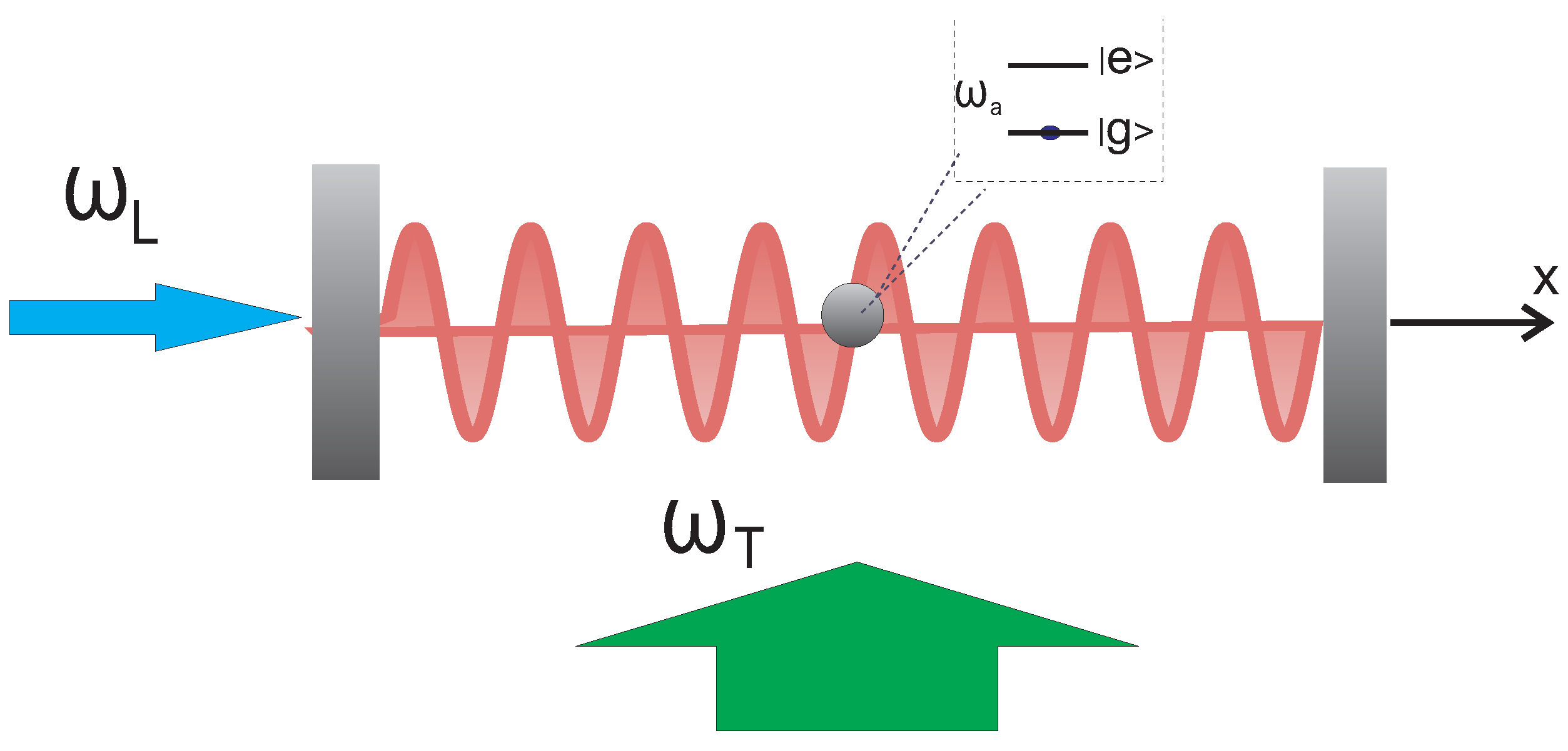
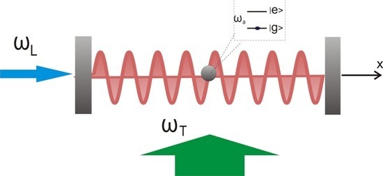
Figure 1) have been theoretically investigated in the limit of equal laser frequencies [
16]; in such a case, in a properly chosen rotating frame the effective combined optical potential can be rendered time independent and the analysis greatly simplifies.
Figure 1.
Schematics. Illustration of the model considered involving an atom moving inside an optical cavity with longitudinal driving of strength and frequency and transverse driving and frequency . The interference between the longitudinally pumped field and the field scattered from the transverse pump into the cavity mode leads to an effective optical potential that has a time dependent part oscillating at the frequency difference .
Here we depart from this scenario to consider frequency beatings between the two pumps. While dynamics in the regime, where each pump acts alone, is well understood, extra forces arise from the interference between photons of different frequencies: (i) scattered from the transverse light field and (ii) entering the cavity mode from the longitudinal pump. The immediate effect of this interference force is to generate a time-dependent optical potential with a time modulation leading to a sign change that effectively induces the particle into undergoing jumps along the cavity sites in a quasi-random walk fashion. We analyze such a regime both numerically and via simplified analytical models. The mechanism is reminiscent of the one exploited in the creation of artificial potentials in optical lattices [
17] applied here to the classical regime. By discretizing the trajectories, we analyze the emerging discrete process via its correlation function and find that it corresponds to an environment with a very short memory. The goal of this analysis is to provide a quantum optical setting in which the classical random walk can be observed and which would constitute a starting point into further generalizations into the quantum regime. In this sense, this work is a stepping stones towards a proposal for implementing a quantum random walk mirroring progress already achieved with photons [
18], atoms in optical lattices [
19], ions in traps [
20] or on a one-dimensional lattice of superconducting qubits [
21]. Our analysis is mainly based on a single two-level system but we discuss as well an extension involving doped micro-spheres where the field addresses a collective atomic variable (along the lines of hybrid optomechanics with doped mechanical resonators [
22]).
The paper is organized as follows: in
Section 2 we introduce the model. In
Section 3 we present numerical evidence showing the occurrence of a quasi-random walk behavior and compute correlations of the engineered process that map close to those expected from a true random walk. In
Section 4, we present a simplified analytical model that allows us to derive the different forces acting on the particle and identify different regimes and associated scalings for the occurrence of the random walk. In
Section 5, we discuss possible extensions of the model involving a tailored driving via a frequency comb laser. We conclude and present an outlook in
Section 6.
2. Model
We consider the effective one-dimensional model depicted depicted in
Figure 1 where an optical cavity mode at
, decaying at rate κ is driven through a side mirror by a laser of amplitude
and frequency
. Transversally, a second laser drives the atom directly with effective amplitude
at
. The longitudinal mode spatial variation inside the cavity is
(
k is the corresponding wave-vector for the light mode with wavelength
) and the atom-photon coupling is specified by
(with
g being the maximum coupling). The total system is described by the Hamiltonian
consisting of a free part
, a pumping term
and the Jaynes-Cummings interaction
. The free evolution Hamiltonian describes the dynamics of a free particle of mass
m and momentum operator
plus that of the cavity mode (annihilation operator
) and the two-level atom
The atom dynamics is described with the help of the Pauli operators
and
satisfying
and
. The atom’s interaction with the cavity field is included as a Jaynes-Cummings photon-excitation exchange process quantified by the position dependent coupling strength
:
Finally driving is included in the pump terms
including direct pumping into mode
and atom driving of the dipole operator
.
We proceed in a standard way to derive equations of motion for classical quantities [
23]. First, we make a set of transformations to dimensionless normalized position
and momentum
. We denote the field amplitude by
and the averaged atomic polarization by
(in a frame rotating at
). In a first stage we consider finite saturations of the population difference operator
whose classical average we denote by
. We furthermore assume that the build-up of quantum correlations between the atom and the photon field can be neglected so that we can replace the nonlinear terms such as
by their factorized classical averages
. The complete equations of motion for atom and field are (including the dissipative dynamics of the field mode at rate κ and of the atomic coherence at rate γ):
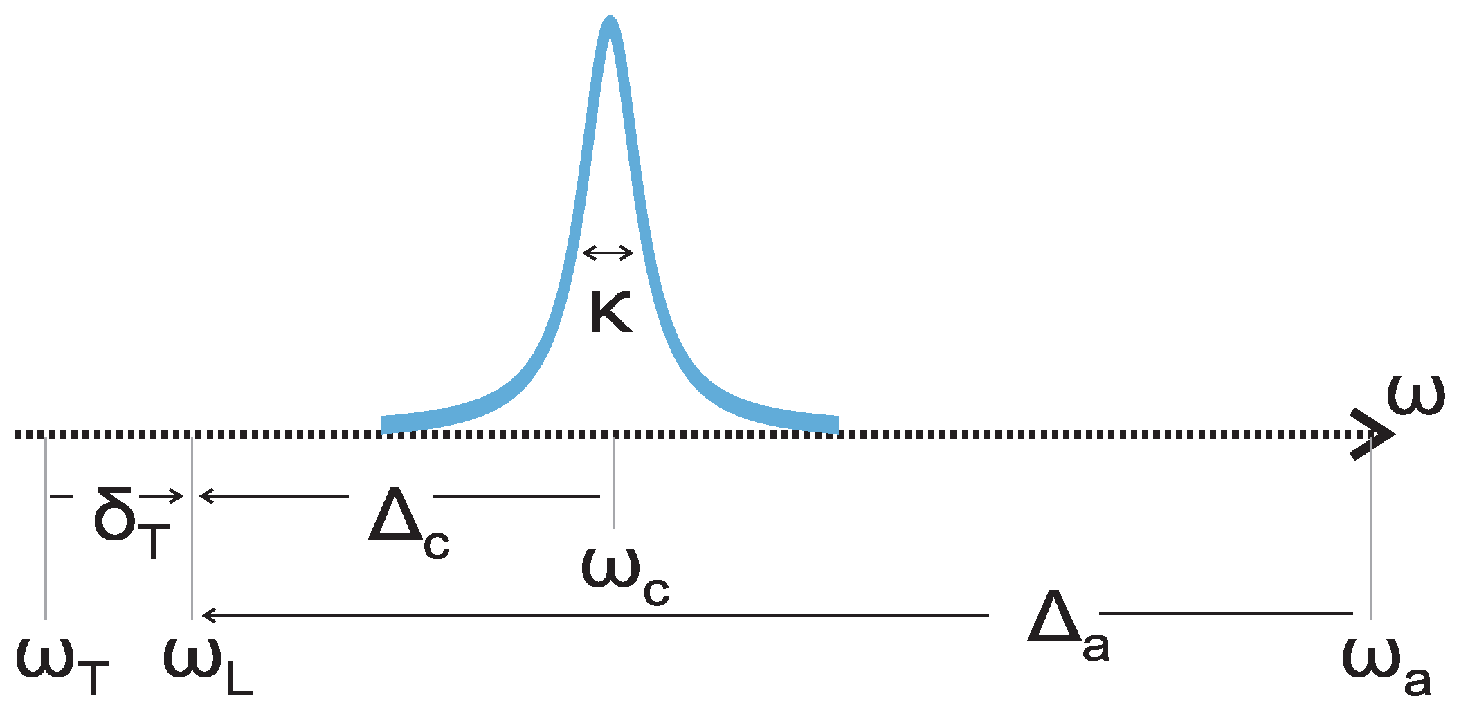
We introduced the detunings
,
and
(illustrated in
Figure 2 with corresponding sign conventions).
Figure 2.
Frequencies. Illustration of the frequencies and detunings as defined/used in the equations of motion. The detunings are taken with respect to the longitudinal driving frequency such that corresponding to the stable regime of cavity QED with moving atoms (far from motional instability points) and that corresponds to as for high-field seekers.
However, for the moment, we restrict our treatment to the low saturation case, where
which allows us to linearize the
term by setting
. Such a linearized regime allows one to analytically derive the forces acting on the particle. Numerical evidence points out that this simplified limit provides similar effects with the finite saturation case and we will base our analytical treatment on the following simplified system of equations:
The motion of the atom is described by
where we have condensed the particle’s properties into the recoil frequency
and we have neglected spontaneous emission induced momentum diffusion.
3. The Quasi-Random Walk—Numerical Results
Before obtaining insight from analytical considerations, we start by simulating the dynamics of the system. This is achieved by fixing the set of parameters to:
,
,
,
,
,
,
and recoil frequency
. We treat
as a free varying parameter. In the following we set
for numerical simulations and normalize the time in units of
. We choose a regime described in the next analytical section as “trapping via longitudinal pump”, where we first tune the parameters such that trapping of the particle is ensured in the absence of the transverse driving. We then increase
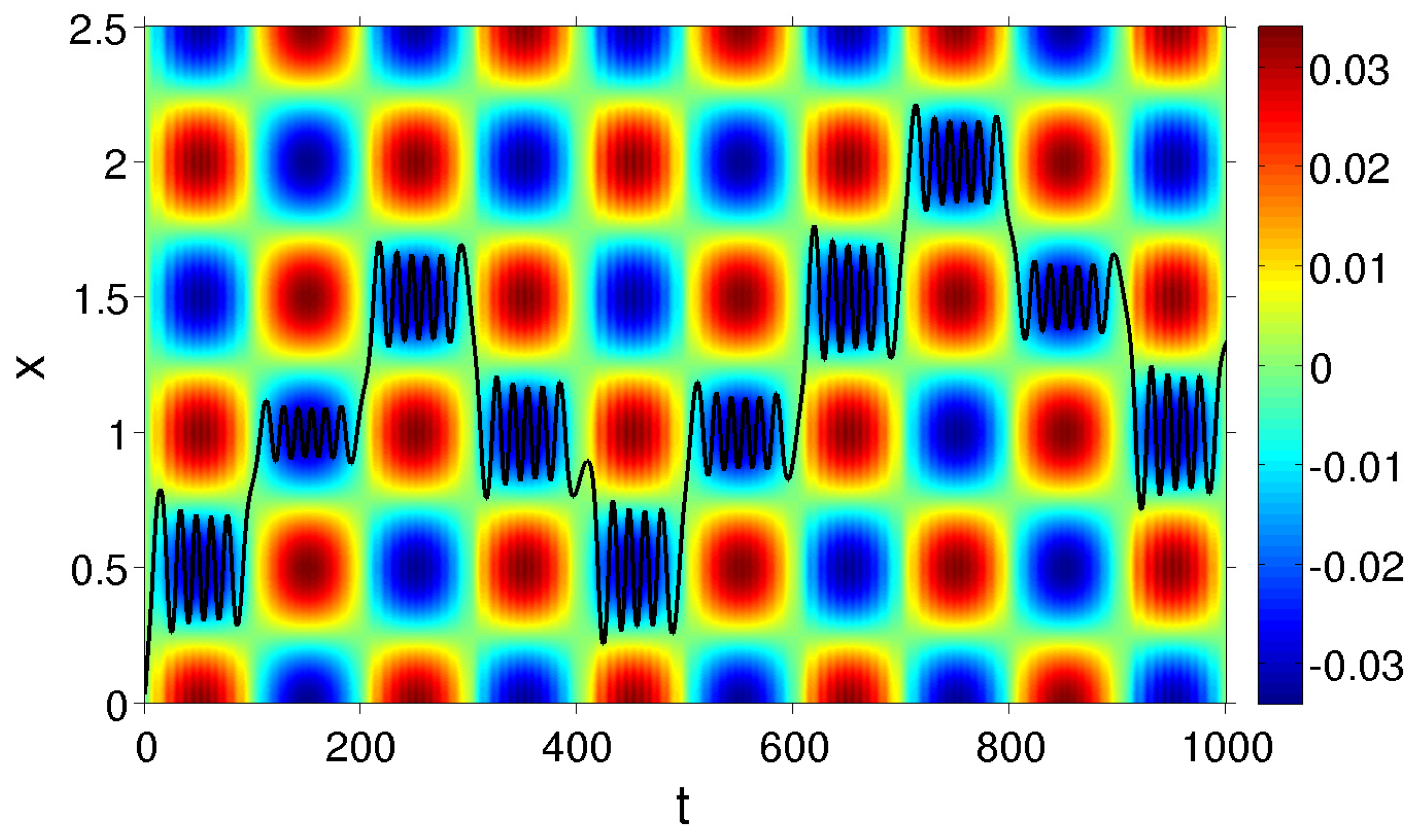
, and notice that past a given threshold, the particle starts jumping out of its trapping site to the neighboring left/right sites in an apparently random way. In
Figure 3 we exemplify such a trajectory obtained for a particle initialized with
around the origin at
and for
.
Figure 3.
Quasi-random walk trajectory. A single trajectory (black curve) overlapped with the effective potential as a function of increasing time for lattice sites appearing at full and half integer values of x (with ). The optical potential is illustrated as colored background and oscillates in time with a period of . Note that t is dimensionless as it is expressed in units of and κ is set to unity.
3.1. Discrete Process—Single Trajectories
We then discretize the process by choosing time steps in units of the time period between two jumps
T, which is half the period of the potential time oscillation. At
the particle is released from the potential and jumps to an adjacent trapping site. This is illustrated in
Figure 4 as the transition from the continuous trajectories in the upper plot to the discrete plots of site number in the middle plot. The discrete positions (the locations of the sites) are defined as:
where the square brackets stand for the rounding of the integral to the nearest integer, corresponding to the location of the site where trapping occurs.
With the parameters from above, we then analyze the dynamics as a function of randomized initial conditions; we initialize the particle with a momentum and position
inside the potential well around zero and follow the evolution over time normalized to
T for
initial values. First, we illustrate the mixing of trajectories, as shown in
Figure 5, by color coding the trajectories starting with
in green and those starting with
in black. The mixing is evident and can be taken as a first indicator for randomness.
Figure 4.
Discretization of the process. (a) Example of a single continuous trajectory plotted versus time and the corresponding discretized position as green dots in the center of one single well oscillation; (b) Corresponding discrete trajectory over 100 jumps, which conform to time units, as a function of the jump index n; (c) Correlation function of the single trajectory from above as a function of time delay between two occurring jumps.
One can introduce the jump sequence
, where the jump indicators are defined as
, and according to their sign show either left or right jump behavior. One can define the autocorrelation function for this process as
which characterizes the joint probability for the occurrence of jumps separated by a time delay
. The behavior of this function for a single trajectory is shown in
Figure 4c in the lower plot. By definition the zero time delay correlation is normalized to unity and it decreases to values around zero where negative values show anti-correlated jumps while positive values indicate correlated jumps.
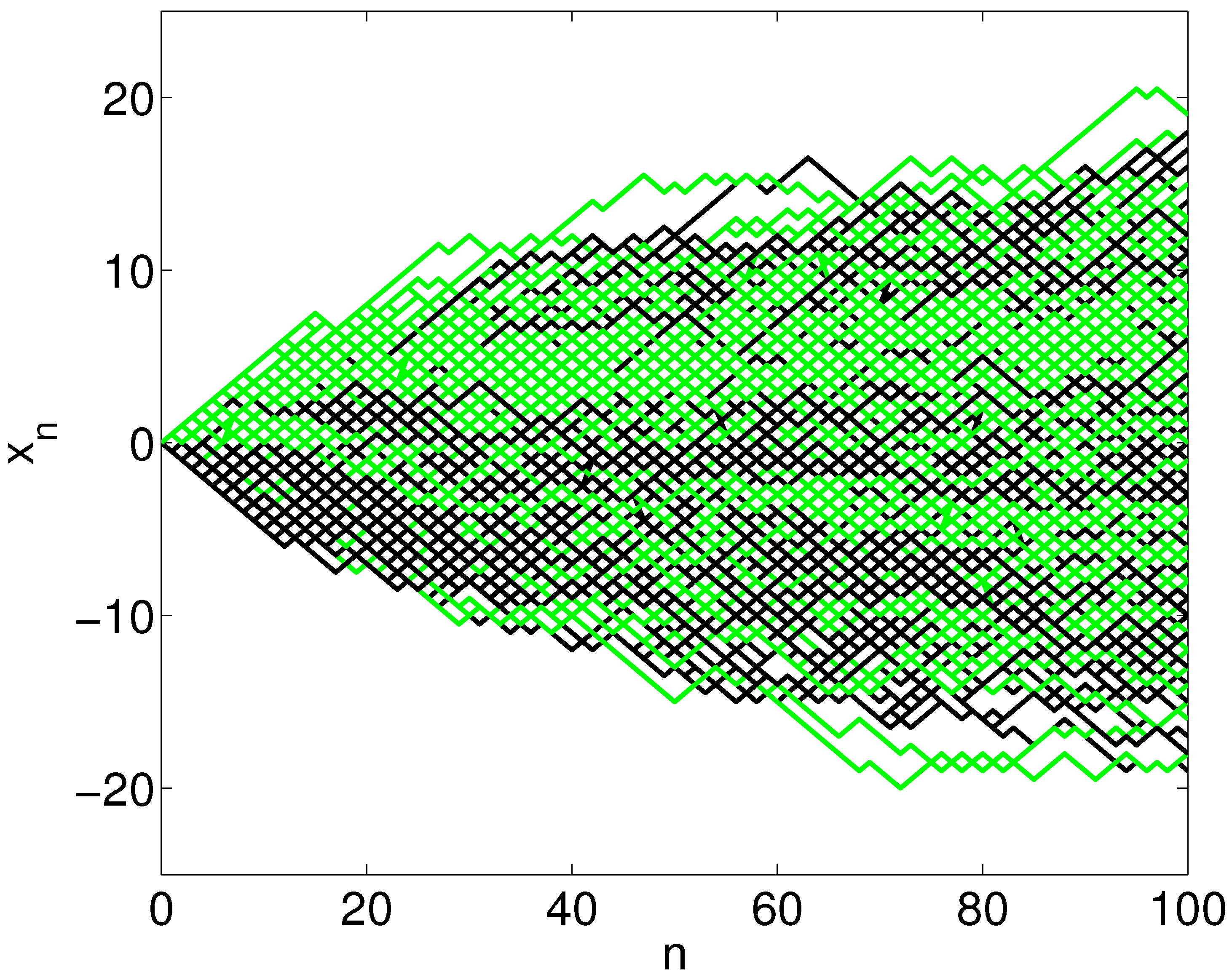
Figure 5.
Mixing of trajectories. Simulation of discrete trajectories as a function of the jump number index n, starting with uniform distributed initial positions and momenta out of the interval . The color coding refers to negative/positive initial positions (black/green): notice that the evolution completely mixes the negative and positive regions.
3.2. Discrete Process—Many Trajectories Statistics
We numerically simulate a large number of trajectories (with starting point around the origin) for
time steps and different values of the jump period
T. The distribution of the final site occupancy is illustrated in
Figure 6a–c. The histograms of all three cases coincide with binomial distributions expected from the classical random walk. The fitting is done with a Gaussian distribution, where the standard deviation of the histogram is considered as the distribution’s width. The variance in position
x of the unbiased binomial distribution is given by
, where
a is the constant spatial separation of adjacent lattice sites. Since the trapping positions in our model are separated by a distance of
and we set
, we expect a variance of
. The numerically observed variances in
Figure 6d–f show a dependency of the slope of the linear increase, which is equivalent to the diffusion constant, on the jump period
T.
Figure 6.
Final site occupancy and mean variances. (a)–(c) Histograms of populations of lattice sites at arrival. The arising distributions fit well with the expected binomial distribution (here the fit is with a Gaussian owing to the large number of steps considered ) characteristic of a random walk. The standard deviations of the distributions vary with the time period T between two jumps. This corresponds to different diffusion constants, given by the slopes of the variance curves below; (d)–(f) Mean variance in position as a function of jump index n. The linear increase with the amount of steps reproduces the main property of a classical discrete one dimensional random walk. For the slope is close to the expected value of for a perfect random walk, while the other two cases show sub-diffusion.
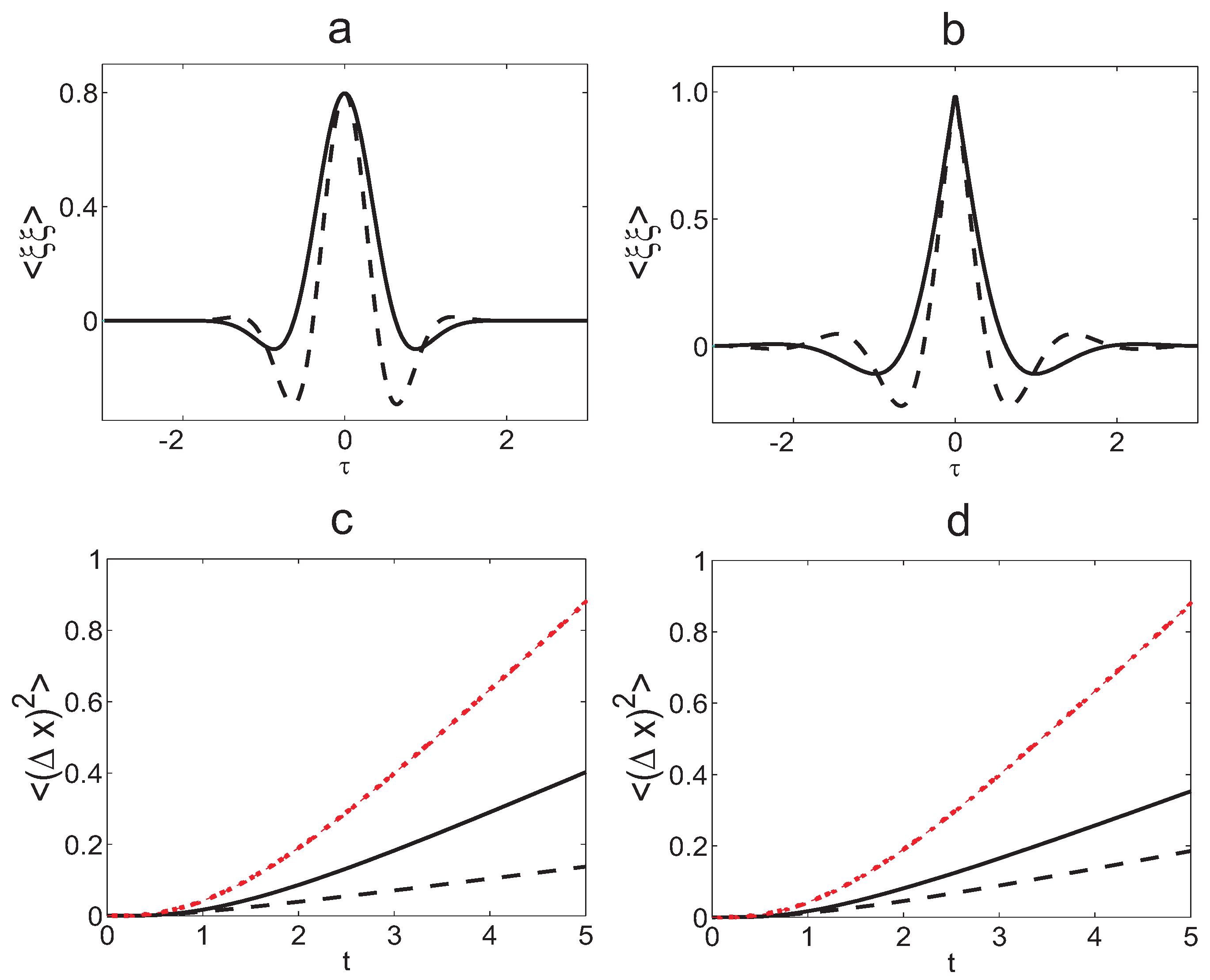
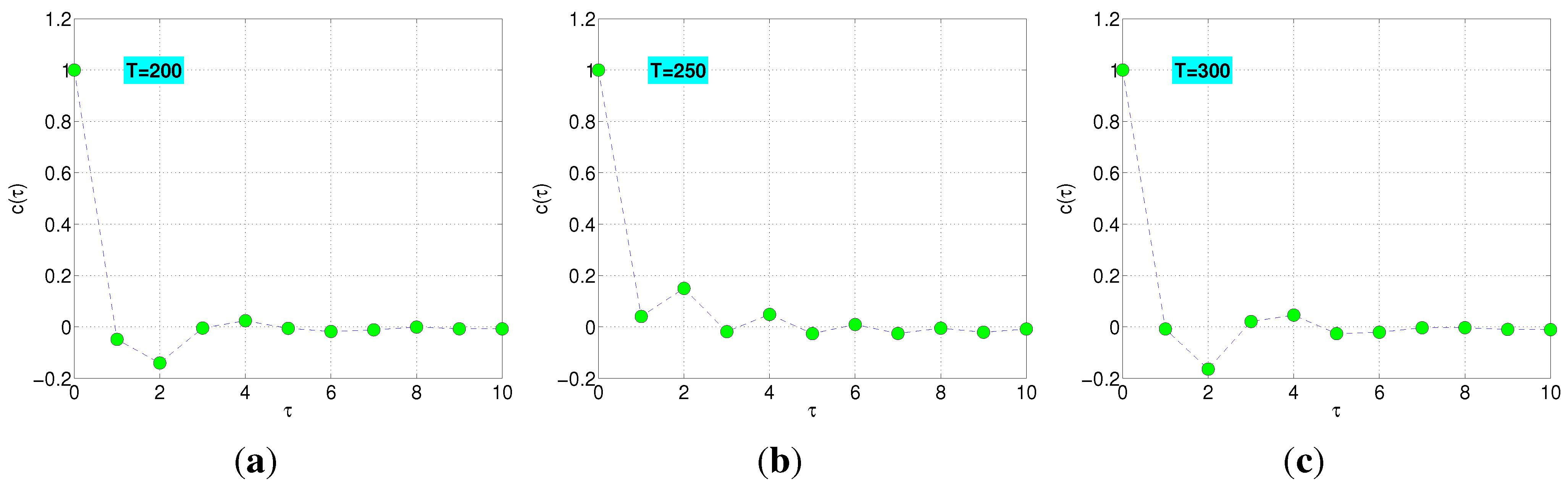
The main result of the numerical section is however the behavior of the jump correlation function averaged over many trajectories (see
Figure 7). For a perfect random walk process, the correlation function for jumps separated by
would be vanishing. This corresponds to a reservoir having no memory. In our case for
and 300 however, short time delays (below 5 jumps) are anti-correlated while after around 5 jumps correlations occur. These anti-correlations do not occur in the second case, which shows the best coincidence with the expectation for a perfect random walk. The anti-correlations seem to correspond to sub-diffusion of the averaged particle motion as they favor jumps back to origin at given time distances which might inhibit the spread of the total motion.
Figure 7.
Averaged jump-correlations. Numerical data showing the variation of the correlation function with the delay time between jumps for different values of T. As a basis of comparison, the correlations of a pure random walk would correspond to a function reaching unity for and zero elsewhere. On the given numerical example, the particle is subjected to an effective reservoir with a non-vanishing memory that allows for anti-correlations of jumps close to each other. These strong negative regions are missing in the middle case b) that corresponds to the highest diffusion.
To gain some physical understanding, one can inspect Equation (11) where the right-hand side represents the effective optical force. In some limit (revealed by the numerical results) this force shows effective quasi-random kicks whose correlations map onto the correlation function for the discrete process. For perfectly uncorrelated kicks the effect would be a random walk. However, in the realistic case some correlations between jumps remain. One can consider the following argument: the momentum kick at one site is the integral of the force over a time T during which the force varies non-trivially. In the continuous limit the process is deterministic. However, in the limit of many oscillations inside a single site, the phases of the momentum kicks occurring at different sites are randomized. On the other hand the numerical results show an alternating behavior of the system with T. The fact that e.g., the diffusion constant decreases again from to gives rise for the hypotheses that this system is more close to a random walk for special ratios of the phases of the single trapping site oscillations and the oscillation of the potential in time.
6. Conclusions and Outlook
We considered the dynamics of particles (either as single two-level systems or sub-micron spheres doped with multiple emitters) inside time-dependent potentials resulting from interference in a two-color, two directional pump scheme. Past a given threshold, chaotic-like behavior can be observed, with correlations very close to those of a typical random walk. Depending on the beat frequency, the particles motion exhibits sub-diffusion that can be related to anti-correlations of the acting force. Analytically the system in the steady state can be reduced to a pendulum with a time dependent frequency modulation.
While the treatment here is in the classical regime, an immediate generalization into the quantum realm can be made by either: (i) treating motion classically and considering the effect of the quantum nature of the two-level system onto the dynamics or (ii) treating motion quantum mechanically and analyzing the dynamics of an initial wave packet, with direct connection to matter-wave interferometry applications. Another future direction aims to extend the 1D treatment to 3D dynamics where the beating of the two pumps give rise to an effective ponderomotive force. Investigations will be carried out on the possibility to exploit such a force for all optical trapping of polarizable particles (or realistic multilevel atoms) inside 3D optical cavities, similar to the mechanism employed in ion trapping inside linear Paul traps.

