Radiative Recombination and Photoionization Data for Tungsten Ions. Electron Structure of Ions in Plasmas

Abstract

Theoretical studies of tungsten ions in plasmas are presented. New calculations of the radiative recombination and photoionization cross-sections, as well as radiative recombination and radiated power loss rate coefficients have been performed for 54 tungsten ions for the range W⁶⁺–W⁷¹⁺. The data are of importance for fusion investigations at the reactor ITER, as well as devices ASDEX Upgrade and EBIT. Calculations are fully relativistic. Electron wave functions are found by the Dirac–Fock method with proper consideration of the electron exchange. All significant multipoles of the radiative field are taken into account. The radiative recombination rates and the radiated power loss rates are determined provided the continuum electron velocity is described by the relativistic Maxwell–Jüttner distribution. The impact of the core electron polarization on the radiative recombination cross-section is estimated for the Ne-like iron ion and for highly-charged tungsten ions within an analytical approximation using the Dirac–Fock electron wave functions. The effect is shown to enhance the radiative recombination cross-sections by ≳20%. The enhancement depends on the photon energy, the principal quantum number of polarized shells and the ion charge. The influence of plasma temperature and density on the electron structure of ions in local thermodynamic equilibrium plasmas is investigated. Results for the iron and uranium ions in dense plasmas are in good agreement with previous calculations. New calculations were performed for the tungsten ion in dense plasmas on the basis of the average-atom model, as well as for the impurity tungsten ion in fusion plasmas using the non-linear self-consistent field screening model. The temperature and density dependence of the ion charge, level energies and populations are considered.

1. Introduction

Experimental and theoretical investigation of tungsten becomes important due to its employment in up-to-date tokamaks. In fusion reactors, the core plasma temperature is expected to be about 25 keV. Tungsten is used as a wall material for the divertor in JET and for the first-wall in ASDEX Upgrade. It is assumed that tungsten will be used as a plasma-facing material in the fusion reactor ITER due to such features as high thermal conductivity, a high melting point, low erosion, low sputtering and low tendency to trap tritium [1–3]. However, tungsten as a high-Z plasma impurity is an efficient radiator at high temperature, and the tungsten influx should be controlled. Because of this, the tungsten radiative characteristics have become the subject of study. Radiative recombination (RR) of tungsten impurity ions with plasma electrons and the inverse process of photoionization of tungsten ions are significant mechanisms that influence the ionization equilibria and the thermal balance of fusion plasmas. Tungsten is also investigated for such devices as ASDEX Upgrade and EBIT to produce data for ITER. In particular, the new active spectroscopy diagnostic of highly-charged ions is applied in studies at EBIT [4]. The diagnostic involves accurate theoretical values of the RR cross-sections for different tungsten ions. However, until recently, the systematic theoretical data on ionization-recombination cross-sections and coefficients for heavy-element ions have been practically unavailable.

Therefore, our purpose was to elaborate a new database, including accurate values of partial and total RR cross-sections (RRCS), partial photoionization cross-sections (PCS), partial and total RR rate coefficients (RR rates) and radiated power loss rate coefficients (RPL rates) for the majority of tungsten ions. We have performed fully relativistic calculations of RRCS and PCS using the Dirac–Fock (DF) method taking into account all significant multipoles of the radiative field for a large number of the heavy element impurity ions, among which are tungsten ions with closed shells, namely, W⁶⁺, W²⁸⁺, W³⁸⁺, W⁴⁶⁺, W⁵⁶⁺, W⁶⁴⁺, as well as W⁷²⁺–W⁷⁴⁺ [5]. Then, calculations of the RR rates for these highly-charged tungsten ions, with the exception of W⁶⁺, have been carried out in a wide temperature range [6]. Analysis of data for tungsten ions and a comparison of our results with available previous calculations are described in [7]. Numerical results of RPL rates for the eight highly-charged tungsten ions are also given in [7].

In the framework of the IAEA Coordinated Research Project (CRP) “Spectroscopic and Collisional Data for Tungsten in Plasma from 1 eV to 20 keV”, we performed new calculations of the RR and photoionization data for additional 54 tungsten ions in the charge range W⁶⁺–W⁷¹⁺ [8–10]. Accurate relativistic values of the partial and total RRCS, partial PCS, as well as partial and total RR/RPL rates were obtained. Total RRCS were calculated in the electron energy range from 1 eV–∼80 keV. Partial PCS and RRCS were fitted by an analytical expression with five fit parameters in the wide photon energy range for all electron states with principal quantum numbers n ≤ 10 and orbital momenta ℓ ≤ 4. Partial RR and RPL rates for the same states and the associated total rates are presented for eleven values of temperature in the range from 10⁴ K–10⁹ K. Values of RR and RPL rates for W⁶⁺ are given in this paper (see

Table A1. Radiative recombination rate coefficients for W⁶⁺ in cm3 × s⁻¹. Presented for a value to its right is the decimal order, e.g., 8.42–13 = 8.42 × 10⁻¹³.

Shell	log10 T (K)
	4.0	4.5	5.0	5.5	6.0	6.5	7.0	7.5	8.0	8.5	9.0
5d3/2	8.42–13	4.54–13	2.26–13	9.38–14	3.30–14	2.23–14	2.36–14	1.57–14	6.29–15	1.68–15	3.16–16
5d5/2	1.14–12	6.12–13	3.02–13	1.24–13	4.44–14	3.26–14	3.43–14	2.22–14	8.64–15	2.26–15	4.17–16
5f5/2	2.02–13	1.01–13	4.22–14	1.34–14	8.99–15	1.21–14	8.25–15	3.08–15	7.78–16	1.53–16	2.38–17
5f7/2	2.59–13	1.29–13	5.35–14	1.70–14	1.23–14	1.66–14	1.12–14	4.15–15	1.04–15	2.04–16	3.17–17
5g7/2	1.10–13	5.35–14	2.17–14	6.90–15	1.74–15	3.75–16	7.35–17	1.36–17	2.40–18	4.02–19	5.90–20
5g9/2	1.38–13	6.73–14	2.73–14	8.67–15	2.19–15	4.73–16	9.26–17	1.71–17	3.03–18	5.07–19	7.44–20
6s1/2	1.83–14	1.07–14	6.75–15	4.79–15	3.94–15	3.62–15	3.35–15	2.77–15	1.89–15	9.96–16	3.73–16
6p1/2	6.71–14	3.63–14	1.85–14	8.55–15	3.91–15	2.61–15	2.66–15	2.41–15	1.52–15	6.50–16	1.84–16
6p3/2	8.69–14	4.73–14	2.46–14	1.26–14	7.61–15	6.71–15	6.61–15	5.19–15	2.86–15	1.08–15	2.74–16
6d3/2	2.66–13	1.43–13	7.02–14	2.86–14	9.62–15	5.72–15	5.87–15	3.92–15	1.57–15	4.22–16	7.92–17
6d5/2	3.78–13	2.02–13	9.87–14	3.97–14	1.35–14	8.59–15	8.75–15	5.66–15	2.22–15	5.81–16	1.07–16
6f5/2	1.78–13	9.01–14	3.82–14	1.22–14	6.13–15	7.32–15	5.02–15	1.89–15	4.78–16	9.38–17	1.47–17
6f7/2	2.30–13	1.16–13	4.88–14	1.55–14	8.23–15	9.96–15	6.75–15	2.52–15	6.33–16	1.24–16	1.93–17
6g7/2	1.25–13	6.11–14	2.48–14	7.89–15	1.99–15	4.29–16	8.40–17	1.55–17	2.75–18	4.60–19	6.76–20
6g9/2	1.57–13	7.65–14	3.11–14	9.90–15	2.50–15	5.40–16	1.06–16	1.95–17	3.46–18	5.80–19	8.51–20
7s1/2	8.09–15	4.82–15	3.10–15	2.20–15	1.72–15	1.48–15	1.34–15	1.10–15	7.48–16	3.95–16	1.48–16
7p1/2	3.97–14	2.12–14	1.05–14	4.60–15	1.96–15	1.20–15	1.17–15	1.05–15	6.64–16	2.83–16	8.01–17
7p3/2	5.18–14	2.76–14	1.38–14	6.59–15	3.66–15	3.04–15	2.94–15	2.31–15	1.28–15	4.82–16	1.22–16
7d3/2	1.49–13	7.95–14	3.88–14	1.56–14	5.12–15	2.84–15	2.84–15	1.89–15	7.60–16	2.04–16	3.83–17
7d5/2	2.16–13	1.15–13	5.56–14	2.21–14	7.28–15	4.30–15	4.25–15	2.75–15	1.08–15	2.82–16	5.21–17
7f5/2	1.32–13	6.70–14	2.86–14	9.14–15	4.06–15	4.48–15	3.06–15	1.15–15	2.92–16	5.74–17	8.98–18
7f7/2	1.72–13	8.67–14	3.67–14	1.17–14	5.41–15	6.07–15	4.10–15	1.53–15	3.86–16	7.56–17	1.18–17
7g7/2	1.09–13	5.31–14	2.16–14	6.88–15	1.74–15	3.75–16	7.34–17	1.36–17	2.41–18	4.04–19	5.96–20
7g9/2	1.37–13	6.65–14	2.71–14	8.64–15	2.18–15	4.71–16	9.23–17	1.71–17	3.02–18	5.06–19	7.43–20
8s1/2	4.31–15	2.62–15	1.73–15	1.23–15	9.27–16	7.73–16	6.84–16	5.60–16	3.80–16	2.01–16	7.51–17
8p1/2	2.65–14	1.39–14	6.67–15	2.82–15	1.14–15	6.58–16	6.24–16	5.59–16	3.53–16	1.50–16	4.25–17
8p3/2	3.49–14	1.83–14	8.82–15	4.00–15	2.09–15	1.66–15	1.58–15	1.24–15	6.85–16	2.59–16	6.56–17
8d3/2	9.38–14	4.99–14	2.41–14	9.59–15	3.10–15	1.65–15	1.61–15	1.07–15	4.32–16	1.16–16	2.17–17
8d5/2	1.38–13	7.31–14	3.50–14	1.37–14	4.45–15	2.50–15	2.43–15	1.57–15	6.13–16	1.61–16	2.97–17
8f5/2	9.63–14	4.88–14	2.09–14	6.68–15	2.77–15	2.90–15	1.97–15	7.44–16	1.89–16	3.71–17	5.80–18
8f7/2	1.25–13	6.34–14	2.69–14	8.56–15	3.68–15	3.92–15	2.64–15	9.88–16	2.49–16	4.88–17	7.62–18
8g7/2	8.83–14	4.31–14	1.76–14	5.59–15	1.41–15	3.04–16	5.95–17	1.11–17	1.99–18	3.40–19	5.09–20
8g9/2	1.11–13	5.40–14	2.20–14	7.01–15	1.77–15	3.82–16	7.48–17	1.38–17	2.47–18	4.19–19	6.21–20
9s1/2	2.57–15	1.59–15	1.06–15	7.57–16	5.59–16	4.55–16	3.98–16	3.25–16	2.21–16	1.16–16	4.35–17
9p1/2	1.88–14	9.71–15	4.55–15	1.87–15	7.30–16	4.03–16	3.73–16	3.33–16	2.10–16	8.96–17	2.53–17
9p3/2	2.50–14	1.29–14	6.04–15	2.64–15	1.32–15	1.01–15	9.53–16	7.45–16	4.11–16	1.55–16	3.93–17
9d3/2	6.32–14	3.35–14	1.61–14	6.33–15	2.02–15	1.04–15	1.01–15	6.70–16	2.70–16	7.23–17	1.36–17
9d5/2	9.38–14	4.95–14	2.35–14	9.13–15	2.92–15	1.59–15	1.52–15	9.81–16	3.84–16	1.01–16	1.86–17
9f5/2	7.12–14	3.60–14	1.54–14	4.93–15	1.96–15	1.97–15	1.34–15	5.05–16	1.28–16	2.52–17	3.94–18
9f7/2	9.29–14	4.69–14	1.99–14	6.33–15	2.60–15	2.66–15	1.79–15	6.70–16	1.69–16	3.31–17	5.17–18
9g7/2	7.02–14	3.43–14	1.40–14	4.43–15	1.12–15	2.41–16	4.74–17	8.92–18	1.61–18	2.72–19	4.00–20
9g9/2	8.78–14	4.29–14	1.75–14	5.56–15	1.41–15	3.03–16	5.95–17	1.11–17	1.99–18	3.36–19	4.94–20
10s1/2	1.65–15	1.04–15	7.04–16	4.99–16	3.63–16	2.90–16	2.52–16	2.06–16	1.39–16	7.35–17	2.75–17
10p1/2	1.39–14	7.10–15	3.25–15	1.30–15	4.95–16	2.65–16	2.42–16	2.15–16	1.35–16	5.77–17	1.63–17
10p3/2	1.86–14	9.46–15	4.33–15	1.83–15	8.83–16	6.58–16	6.18–16	4.83–16	2.66–16	1.01–16	2.55–17
10d3/2	4.50–14	2.37–14	1.13–14	4.40–15	1.39–15	7.05–16	6.75–16	4.48–16	1.80–16	4.83–17	9.07–18
10d5/2	6.71–14	3.52–14	1.66–14	6.38–15	2.02–15	1.07–15	1.02–15	6.55–16	2.56–16	6.73–17	1.24–17
10f5/2	5.38–14	2.72–14	1.16–14	3.70–15	1.43–15	1.40–15	9.49–16	3.58–16	9.10–17	1.79–17	2.80–18
10f7/2	7.04–14	3.54–14	1.50–14	4.76–15	1.90–15	1.89–15	1.27–15	4.74–16	1.20–16	2.35–17	3.66–18
10g7/2	5.60–14	2.72–14	1.11–14	3.52–15	8.88–16	1.94–16	3.80–17	7.03–18	1.24–18	2.08–19	3.05–20
10g9/2	6.98–14	3.40–14	1.39–14	4.41–15	1.11–15	2.41–16	4.76–17	8.94–18	1.60–18	2.69–19	3.96–20
Total	2.13–11	7.34–12	2.66–12	8.81–13	3.04–13	2.11–13	1.77–13	1.03–13	4.22–14	1.30–14	3.03–15

and

Table A2. Radiated power loss rate coefficients for W⁶⁺ in Watts × cm³. Presented for a value to its right is the decimal order, e.g., 8.75–30 = 8.75 × 10⁻³⁰.

Shell	log10 T (K)
	4.0	4.5	5.0	5.5	6.0	6.5	7.0	7.5	8.0	8.5	9.0
5d3/2	8.75–30	4.84–30	2.57–30	1.22–30	6.56–31	1.76–30	4.78–30	6.47–30	4.82–30	2.20–30	6.48–31
5d5/2	1.16–29	6.42–30	3.39–30	1.59–30	9.11–31	2.62–30	6.82–30	8.88–30	6.37–30	2.78–30	7.80–31
5f5/2	1.03–30	5.42–31	2.46–31	9.77–32	2.70–31	8.47–31	1.04–30	6.32–31	2.32–31	5.90–32	1.08–32
5f7/2	1.32–30	6.92–31	3.11–31	1.26–31	3.76–31	1.16–30	1.40–30	8.39–31	3.05–31	7.67–32	1.39–32
5g7/2	3.62–31	1.88–31	8.70–32	3.36–32	1.09–32	3.14–33	8.09–34	1.83–34	3.62–35	6.37–36	9.54–37
5g9/2	4.53–31	2.36–31	1.09–31	4.23–32	1.37–32	3.96–33	1.02–33	2.31–34	4.57–35	8.05–36	1.20–36
6s1/2	1.60–31	9.75–32	6.88–32	6.78–32	1.10–31	2.60–31	6.77–31	1.56–30	2.87–30	3.95–30	3.76–30
6p1/2	4.98–31	2.79–31	1.57–31	9.19–32	7.78–32	1.79–31	5.82–31	1.37–30	2.04–30	1.94–30	1.21–30
6p3/2	6.17–31	3.49–31	2.02–31	1.39–31	1.82–31	4.87–31	1.35–30	2.65–30	3.38–30	2.76–30	1.44–30
6d3/2	1.39–30	7.85–31	4.37–31	2.22–31	1.31–31	4.03–31	1.16–30	1.60–30	1.20–30	5.50–31	1.62–31
6d5/2	1.96–30	1.10–30	6.07–31	3.04–31	1.90–31	6.16–31	1.69–30	2.25–30	1.63–30	7.14–31	2.01–31
6f5/2	5.91–31	3.20–31	1.55–31	6.26–32	1.51–31	4.98–31	6.28–31	3.86–31	1.43–31	3.63–32	6.65–33
6f7/2	7.62–31	4.12–31	1.98–31	8.03–32	2.08–31	6.73–31	8.36–31	5.08–31	1.86–31	4.68–32	8.49–33
6g7/2	2.91–31	1.55–31	7.55–32	3.09–32	1.06–32	3.18–33	8.48–34	1.95–34	3.91–35	6.91–36	1.04–36
6g9/2	3.64–31	1.95–31	9.47–32	3.88–32	1.33–32	4.01–33	1.07–33	2.47–34	4.93–35	8.72–36	1.31–36
7s1/2	3.97–32	2.52–32	1.98–32	2.25–32	3.97–32	9.84–32	2.63–31	6.14–31	1.13–30	1.56–30	1.49–30
7p1/2	1.72–31	9.76–32	5.60–32	3.42–32	3.09–32	7.50–32	2.50–31	5.91–31	8.85–31	8.44–31	5.26–31
7p3/2	2.17–31	1.23–31	7.25–32	5.20–32	7.33–32	2.08–31	5.89–31	1.17–30	1.50–30	1.23–30	6.42–31
7d3/2	4.95–31	2.86–31	1.67–31	9.04–32	5.69–32	1.88–31	5.51–31	7.69–31	5.80–31	2.66–31	7.85–32
7d5/2	7.14–31	4.10–31	2.37–31	1.26–31	8.43–32	2.90–31	8.12–31	1.09–30	7.90–31	3.47–31	9.76–32
7f5/2	3.09–31	1.73–31	8.84–32	3.72–32	8.75–32	2.97–31	3.81–31	2.36–31	8.75–32	2.23–32	4.10–33
7f7/2	4.00–31	2.23–31	1.13–31	4.77–32	1.20–31	4.01–31	5.05–31	3.09–31	1.13–31	2.86–32	5.20–33
7g7/2	1.89–31	1.04–31	5.33–32	2.30–32	8.21–33	2.56–33	7.00–34	1.67–34	4.14–35	1.20–35	2.71–36
7g9/2	2.37–31	1.31–31	6.69–32	2.89–32	1.03–32	3.23–33	8.84–34	2.06–34	4.15–35	7.35–36	1.10–36
8s1/2	1.38–32	9.24–33	8.06–33	1.03–32	1.94–32	4.91–32	1.33–31	3.11–31	5.76–31	7.95–31	7.57–31
8p1/2	7.64–32	4.38–32	2.58–32	1.65–32	1.56–32	3.90–32	1.32–31	3.13–31	4.69–31	4.48–31	2.79–31
8p3/2	9.80–32	5.61–32	3.37–32	2.52–32	3.74–32	1.09–31	3.14–31	6.29–31	8.07–31	6.59–31	3.45–31
8d3/2	2.19–31	1.30–31	7.97–32	4.57–32	3.03–32	1.05–31	3.11–31	4.35–31	3.29–31	1.51–31	4.46–32
8d5/2	3.20–31	1.89–31	1.14–31	6.44–32	4.54–32	1.62–31	4.59–31	6.18–31	4.49–31	1.97–31	5.56–32
8f5/2	1.68–31	9.72–32	5.24–32	2.30–32	5.46–32	1.89–31	2.45–31	1.52–31	5.65–32	1.44–32	2.64–33
8f7/2	2.19–31	1.26–31	6.72–32	2.95–32	7.50–32	2.55–31	3.24–31	1.99–31	7.32–32	1.85–32	3.36–33
8g7/2	1.20–31	6.85–32	3.66–32	1.65–32	6.12–33	1.96–33	5.55–34	1.74–34	7.36–35	3.25–35	8.79–36
8g9/2	1.51–31	8.57–32	4.59–32	2.08–32	7.71–33	2.47–33	6.91–34	1.83–34	6.29–35	2.35–35	2.63–36
9s1/2	5.82–33	4.14–33	4.00–33	5.63–33	1.10–32	2.82–32	7.67–32	1.80–31	3.34–31	4.61–31	4.39–31
9p1/2	3.90–32	2.27–32	1.38–32	9.15–33	9.00–33	2.30–32	7.80–32	1.86–31	2.79–31	2.67–31	1.66–31
9p3/2	5.07–32	2.94–32	1.82–32	1.41–32	2.18–32	6.48–32	1.88–31	3.77–31	4.84–31	3.96–31	2.07–31
9d3/2	1.10–31	6.73–32	4.35–32	2.62–32	1.82–32	6.48–32	1.93–31	2.72–31	2.05–31	9.43–32	2.79–32
9d5/2	1.63–31	9.90–32	6.29–32	3.72–32	2.73–32	1.01–31	2.86–31	3.86–31	2.81–31	1.24–31	3.48–32
9f5/2	9.73–32	5.80–32	3.28–32	1.49–32	3.62–32	1.27–31	1.65–31	1.03–31	3.84–32	9.80–33	1.79–33
9f7/2	1.27–31	7.53–32	4.22–32	1.92–32	4.97–32	1.71–31	2.19–31	1.35–31	4.97–32	1.26–32	2.27–33
9g7/2	7.74–32	4.55–32	2.55–32	1.20–32	4.57–33	1.50–33	4.82–34	1.74–34	4.56–35	8.84–36	1.36–36
9g9/2	9.68–32	5.70–32	3.19–32	1.50–32	5.75–33	1.89–33	5.70–34	1.84–34	4.83–35	9.51–36	1.48–36
10s1/2	2.82–33	2.13–33	2.26–33	3.41–33	6.84–33	1.77–32	4.83–32	1.14–31	2.11–31	2.91–31	2.77–31
10p1/2	2.20–32	1.30–32	8.15–33	5.60–33	5.68–33	1.47–32	5.02–32	1.20–31	1.80–31	1.72–31	1.07–31
10p3/2	2.90–32	1.71–32	1.08–32	8.68–33	1.38–32	4.17–32	1.21–31	2.44–31	3.13–31	2.56–31	1.34–31
10d3/2	6.13–32	3.86–32	2.61–32	1.64–32	1.18–32	4.29–32	1.29–31	1.81–31	1.37–31	6.29–32	1.86–32
10d5/2	9.11–32	5.70–32	3.80–32	2.34–32	1.78–32	6.67–32	1.91–31	2.58–31	1.88–31	8.26–32	2.32–32
10f5/2	5.95–32	3.66–32	2.16–32	1.02–32	2.52–32	8.96–32	1.17–31	7.31–32	2.72–32	6.95–33	1.27–33
10f7/2	7.79–32	4.77–32	2.79–32	1.31–32	3.46–32	1.20–31	1.55–31	9.54–32	3.52–32	8.89–33	1.62–33
10g7/2	5.12–32	3.11–32	1.82–32	8.85–33	3.45–33	1.09–33	2.59–34	5.11–35	9.22–36	1.55–36	2.28–37
10g9/2	6.39–32	3.89–32	2.28–32	1.11–32	4.35–33	1.47–33	5.11–34	1.53–34	3.38–35	6.11–36	9.19–37
Total	4.12–29	2.20–29	1.15–29	5.55–30	4.82–30	1.41–29	3.05–29	4.02–29	3.65–29	2.60–29	1.52–29

in Appendix). Now, the part of our database concerning tungsten contains data for 62 ions from the range W⁶⁺–W⁷⁴⁺. The results were added to our extended unified database containing the RR and photoionization data for about 170 heavy element impurity ions occurring in fusion plasmas. New data were included in the IAEA Atomic and Molecular database [11].

With the context of CRP, we estimated also an impact of the target core electron polarization following the RR process on RRCS outside the regions of the dielectronic recombination resonances, i.e., the so-called polarization RR effect (PRR effect). Calculations were carried out in the framework of the analytical “stripping” approximation using the relativistic DF electron wave functions. The approximation was shown to provide a reasonable estimation of the PRR effect.

The effect was considered for the Fe XVII ion where a comparison with experimental data was performed [12]. The experimental values of the electron-impact excitation cross-section (EIECS) were determined in [13] by normalizing to measured intensities of the RR peaks, which were independently normalized to the associated theoretical RRCS. The experimental EIECS turned out to be lower by ∼25% as compared to all available theoretical values. We showed that the problem with the determination of absolute values of the measured EIECS was that only the RR channel was taken into account in theoretical RRCS used for normalization, while the PRR channel was overlooked. The inclusion of the PRR channel eliminates this puzzling discrepancy between experimental and theoretical EIECS.

Then, the PRR effect was assessed for the tungsten highly-charged ions [14]. It was obtained that enhancement factor F_n changes from ∼15% to ≲1%. We showed that the factor F_n depends on the photon energy, the principal quantum number of polarized shells and the ion charge, but is practically independent of the final electron state in the RR process.

We studied also an electron structure of ions in local thermodynamic equilibrium (LTE) plasmas [15]. The influence of plasma temperature and density on the energy spectrum and level populations of an ion in dense and fusion plasmas was considered. The code PLASMASATOM was designed on the basis of our computer program complex RAINE (Relativistic atom. Interaction of electromagnetic radiation and nucleus with atomic electrons) [16–18]. The electron wave functions were calculated by the Dirac–Slater (DS) method with approximate consideration for the electron exchange. The code is of the type of the Los Alamos INFERNO code [19,20] and PURGATORIOcode [21], as well as more advanced PARADISIO code [22]. Our results concerning the ionization charges of iron and uranium ions are shown to be in a good agreement with data of previous calculations. New results were obtained for the impurity tungsten ion in fusion plasmas at low temperatures using the non-linear self-consistent field screening model and for the dense tungsten plasmas in the wide temperature range using the average-atom model.

2. Radiative Recombination and Photoionization Data

2.1. Method of Calculations

The exact relativistic treatment of the photoionization process having regard to all multipoles of the radiative field leads to the following expressions for PCS in the i-th atomic subshell [5]:

$${\sigma }_{\mathrm{ph}}^{(i)}=\frac{4{\pi }^2\alpha }{k(2j_i+1)}{\displaystyle \sum _L{\displaystyle \sum _k\left[(2L+1)Q_{LL}^2(k)+L{Q}_{L+1L}^2(k)+(L+1)Q_{L-1L}^2(k)-2\sqrt{L(L+1)}{Q}_{L-1L}(k)Q_{L+1L}(k)\right]}}$$

(1)

Here, k is the photon energy, L is the multipolarity of the radiative field, κ = (ℓ − j)(2j + 1) is the relativistic quantum number, j and ℓ are the total and orbital momentum of the electron and α is the fine structure constant. Equation (1) is written per one electron. Relativistic units (ħ = m₀ = c = 1) are used in equations throughout this text, unless otherwise specified. The reduced matrix element Q_ΛL(κ) has the form:

$$\begin{array}{r}{Q}_{\mathrm{\Lambda }L}(k)={[(2\overline{\mathrm{\ell }}+1)(2{\mathrm{\ell }}_i+1)/(2\mathrm{\Lambda }+1)]}^{1/2}{C}_{\overline{\mathrm{\ell }}0{\mathrm{\ell }}_{i}0}^{\mathrm{\Lambda }0}\mathcal{A}\left(\begin{array}{lll}\overline{\mathrm{\ell }}\hfill & 1/2\hfill & j\hfill \\ {\mathrm{\ell }}_i\hfill & 1/2\hfill & j_i\hfill \\ \mathrm{\Lambda }\hfill & 1\hfill & L\hfill \end{array}\right)R_{1\mathrm{\Lambda }}\\ +{[(2\mathrm{\ell }+1)(2{\overline{\mathrm{\ell }}}_i+1)/(2\mathrm{\Lambda }+1)]}^{1/2}{C}_{\mathrm{\ell }0{\overline{\mathrm{\ell }}}_{i}0}^{\mathrm{\Lambda }0}\mathcal{A}\left(\begin{array}{lll}\mathrm{\ell }\hfill & 1/2\hfill & j\hfill \\ \overline{\mathrm{\ell }}\hfill & 1/2\hfill & j_i\hfill \\ \mathrm{\Lambda }\hfill & 1\hfill & L\hfill \end{array}\right)R_{2\mathrm{\Lambda }}\end{array}$$

(2)

where $\overline{\mathrm{\ell }}=2j-\mathrm{\ell },C_{{\mathrm{\ell }}_{1}0{\mathrm{\ell }}_{2}0}^{\mathrm{\Lambda }0}$ is the Clebsch–Gordan coefficient and $\mathcal{A}\left(\begin{array}{lll}{\mathrm{\ell }}_1\hfill & 1/2\hfill & j_1\hfill \\ {\mathrm{\ell }}_2\hfill & 1/2\hfill & j_2\hfill \\ \mathrm{\Lambda }\hfill & 1\hfill & L\hfill \end{array}\right)$ is the recoupling coefficient for four angular momenta. Radial integrals R_1Λ and R_2Λ are given by:

$$\begin{array}{l}{R}_{1\mathrm{\Lambda }}={\displaystyle \underset{0}{\overset{\infty }{\int }}{G}_i(r)}F(r)j_{\mathrm{\Lambda }}(\mathrm{kr})dr\\ R_{2\mathrm{\Lambda }}={\displaystyle \underset{0}{\overset{\infty }{\int }}G}(r)F_i(r)j_{\mathrm{\Lambda }}(\mathrm{kr})dr\end{array}$$

(3)

where G(r) and F (r) are the large and small components of the Dirac electron wave function multiplied by r and j_Λ(kr) is the spherical Bessel function of the Λ-th order. The subscript i ≡ n_iℓ_ij_i ≡ n_iκ_i relates to the bound electron state, while designations with no subscript relate to the continuum state. The electron wave functions are calculated in the framework of the DF method where the exchange electron interaction is included exactly both between bound electrons and between bound and free electrons [18]. The bound and continuum wave functions are calculated in the self-consistent fields (SCF) of the corresponding ions with N + 1 and N electrons, respectively.

The partial RRCS ${\sigma }_{\mathrm{rr}}^{(i)}$ for a recombining ion W^(q−1)+, as an example, can be expressed in terms of PCS ${\sigma }_{\mathrm{ph}}^{(i)}$ for the associated recombined ion W^(q−1)+, which makes up as the recombining ion with one additional electron in the i-th subshell with quantum numbers n_i, ℓ_i and j_i:

$$W^{(q-1)+}=W^{q+}+(n_i{\mathrm{\ell }}_i{j}_i)$$

(4)

We use the relativistic relationship between PCS and RRCS, which may be written as [23]:

$${\sigma }_{\mathrm{rr}}^{(i)}=\frac{k^2}{2m_0{c}^2{E}_{\mathrm{k}}+E_{\mathrm{k}}^2}{q}^{(i)}{\sigma }_{\mathrm{ph}}^{(i)}$$

(5)

where E_k is the kinetic electron energy and q⁽ⁱ⁾ is the number of vacancies in the i-th subshell prior to recombination.

The relativistic RR rates ${\sigma }_{\text{rel}}^{(i)}(T)$ can be found using the thermal average over the relativistic RRCS/PCS provided the continuum electron velocity is described by the relativistic Maxwell–Jüttner distribution. The associated distribution function f(E) normalized to unity is written as follows [24]

$$f(E)dE=\frac{E{(E^2-1)}^{1/2}}{\theta \exp (1/\theta )K_2(1/\theta )}\times \exp [-(E-1)/\theta ]dE$$

(6)

Here, E is the total electron energy in units of m₀c², including the rest energy, θ = k_βT/m₀c² is the characteristic dimensionless temperature, k_β is the Boltzmann constant and T is the temperature. The modified Bessel function of the second order is denoted by K₂.

Taking account of the relativistic distribution (Equation (6)) along with the relativistic relationship (Equation (5)), the expression for the relativistic RR rates takes the factorized form:

$${\sigma }_{\text{rel}}^{(i)}(T)=<v{\sigma }_{\mathrm{rr}}^{(i)}>=F_{\text{rel}}(\theta )\cdot {\sigma }^{(i)}(T)$$

(7)

Here, v = (p/E)c is the electron velocity with the momentum $p=\sqrt{E^2-1}$. The factor α⁽ⁱ⁾(T) is the usual RR rate with the non-relativistic Maxwell–Boltzmann distribution, which can be written as:

$${\alpha }^{(i)}(T)={(2/\pi )}^{1/2}{c}^{-2}{(m_0{k}_{\beta }T)}^{-3/2}{q}^{(i)}{\displaystyle \underset{{\epsilon }_i}{\overset{\infty }{\int }}{k}^2{\sigma }_{\mathrm{ph}}^{(i)}(k)}{e}^{({\epsilon }_i-k)/(k_{\beta }T)}dk$$

(8)

where ε_i is the ionization threshold energy of the i-th subshell. According to Equation (7), to obtain the relativistic RR rates, α⁽ⁱ⁾(T), involving relativistic values of ${\sigma }_{\mathrm{ph}}^{(i)}(k)$, should be multiplied by the relativistic factor F_rel(θ), which is written as:

$$F_{\text{rel}}(\theta )=\sqrt{\frac{\pi }{2}}\theta /K_2(1/\theta )\exp (1/\theta )$$

(9)

This is just the factor that comes from the relativistic Maxwell–Jüttner distribution with allowance made for relativistic relationship between PCS and RRCS. The factor has been obtained for the first time by us [6,7,25]. It has been taken into consideration in all our calculations of RR/RPL rates.

Similarly, the expression for relativistic RPL rates can be found as:

$${\gamma }_{\text{rel}}^{(i)}(T)=\langle vk{\sigma }_{\mathrm{rr}}^{(i)}\rangle =F_{\text{rel}}(\theta )\cdot {\gamma }^{(i)}(T)$$

(10)

Here, γ⁽ⁱ⁾(T) is the RPL rate obtained using the non-relativistic Maxwell–Boltzmann electron distribution:

$${\gamma }^{(i)}(T)={(2/\pi )}^{1/2}{c}^{-2}{(m_0{k}_{\beta }T)}^{-3/2}{q}^{(i)}{\displaystyle \underset{{\epsilon }_i}{\overset{\infty }{\int }}{k}^3}{\sigma }_{\mathrm{ph}}^{(i)}(k)e^{({\epsilon }_i-k)/(k_{\beta }T)}dk$$

(11)

Note once again that Equations (8) and (11) have to involve relativistic values of PCS. Numerical methods used for calculations of integrals in Equations (8) and (11) are described at length in [7].

2.2. Results and Discussion

The influence of relativistic, non-dipole and exchange effects on PCS, RRCS and RR/RPL rates was considered in [7,25]. It is significant that relativistic and non-dipole effects are of importance for highly-charged ions and at high energies. For example, as is evident from Figure 1, where the factor F_rel(θ) is displayed versus temperature, the relativistic Maxwell–Jüttner distribution decreases RR/RPL rates considerably at a high temperature as compared with the commonly-used non-relativistic Maxwell–Boltzmann distribution. For example, the decreasing is ∼25% at the highest temperature in our calculations T = 10⁹ K ≈ 86 keV.

On the contrary, the exact consideration of the electron exchange is of importance in the RR and photoionization calculations for low-charged ions, especially at low energies. Partial RRCS for recombination of W⁶⁺ with an electron captured in the 5d_3/2, 5f_5/2 and 6p_1/2 states calculated by the DF method having regard to the exact exchange (red curves) and by the DS method having regard to the approximate exchange according to Slater (blue curves) [16] are presented in Figure 2. As is seen, there is a significant difference between the two calculations especially at low electron energies and in the vicinity of the Cooper minimum. The exact consideration of the electron exchange may change partial RRCS and PCS by several times at electron energies E_k ≲ 1, 000 eV and up by ∼70% at high electron energies.

Calculations were performed for the most stable tungsten ions. For each ion, the electron configuration with the lowest total energy was found by the DF method taking into account the Breit magnetic interaction between electrons. It should be noted that all ion configurations obtained by us coincide with those presented in compilation [26], where the experimentally-derived energy levels are used. The adopted electron configuration for 54 ions considered in the framework of CRP are listed in

Table 1. Electron configurations adopted for tungsten ions along with total energies calculated by the DF method taking into account the Breit magnetic interaction between electrons.

Ion	Configuration	−Etot (eV)	Ion	Configuration	−Etot (eV)
W6+	$[\mathrm{Xe}]4f_{5/2}^{6}4f_{7/2}^8$	438,971.5	W42+	$[\mathrm{Ar}]3d_{3/2}^{4}3d_{5/2}^{6}4s^{2}4p_{1/2}^2$	407,964.5
W14+	$[\mathrm{Kr}]4d_{3/2}^{4}4d_{5/2}^{6}4f_{5/2}^{6}4f_{7/2}^{6}5s_{1/2}^2$	437,397.8	W43+	$[\mathrm{Ar}]3d_{3/2}^{4}3d_{5/2}^{6}4s^{2}4p_{1/2}^1$	405,819.8
W15+	$[\mathrm{Kr}]4d_{3/2}^{4}4d_{5/2}^{6}4f_{5/2}^{6}4f_{7/2}^{6}5s_{1/2}^2$	437,072.6	W44+	$[\mathrm{Ar}]3d_{3/2}^{4}3d_{5/2}^{6}4s^2$	403,613.8
W16+	$[\mathrm{Kr}]4d_{3/2}^{4}4d_{5/2}^{6}4f_{5/2}^{6}4f_{7/2}^{6}5s_{1/2}^1$	436,712.7	W45+	$[\mathrm{Ar}]3d_{3/2}^{4}3d_{5/2}^{6}4s^1$	401,260.9
W17+	$[\mathrm{Kr}]4d_{3/2}^{4}4d_{5/2}^{6}4f_{5/2}^{6}4f_{7/2}^5$	436,327.5	W47+	$[\mathrm{Ar}]3d_{3/2}^{4}3d_{5/2}^5$	394,795.1
W18+	$[\mathrm{Kr}]4d_{3/2}^{4}4d_{5/2}^{6}4f_{5/2}^{6}4f_{7/2}^4$	435,907.9	W48+	$[\mathrm{Ar}]3d_{3/2}^{4}3d_{5/2}^4$	390,616.1
W19+	$[\mathrm{Kr}]4d_{3/2}^{4}4d_{5/2}^{6}4f_{5/2}^{6}4f_{7/2}^3$	435,448.6	W49+	$[\mathrm{Ar}]3d_{3/2}^{4}3d_{5/2}^3$	386,307.9
W20+	$[\mathrm{Kr}]4d_{3/2}^{4}4d_{5/2}^{6}4f_{5/2}^{6}4f_{7/2}^2$	434,948.3	W50+	$[\mathrm{Ar}]3d_{3/2}^{4}3d_{5/2}^2$	381,869.1
W21+	$[\mathrm{Kr}]4d_{3/2}^{4}4d_{5/2}^{6}4f_{5/2}^{6}4f_{7/2}^1$	434,405.8	W51+	$[\mathrm{Ar}]3d_{3/2}^{4}3d_{5/2}^1$	377,298.0
W22+	$[\mathrm{Kr}]4d_{3/2}^{4}4d_{5/2}^{6}4f_{5/2}^6$	433,819.9	W52+	$[\mathrm{Ar}]3d_{3/2}^4$	372,593.2
W23+	$[\mathrm{Kr}]4d_{3/2}^{4}4d_{5/2}^{6}4f_{5/2}^5$	433,181.3	W53+	$[\mathrm{Ar}]3d_{3/2}^3$	367,673.9
W24+	$[\mathrm{Kr}]4d_{3/2}^{4}4d_{5/2}^{6}4f_{5/2}^4$	432,496.8	W54+	$[\mathrm{Ar}]3d_{3/2}^2$	362,615.4
W25+	$[\mathrm{Kr}]4d_{3/2}^{4}4d_{5/2}^{6}4f_{5/2}^3$	431,765.3	W55+	$[\mathrm{Ar}]3d_{3/2}^1$	357,416.2
W26+	$[\mathrm{Kr}]4d_{3/2}^{4}4d_{5/2}^{6}4f_{5/2}^2$	430,985.6	W57+	$[\mathrm{Ne}]3s^{2}3p_{1/2}^{2}3p_{3/2}^3$	346,348.4
W27+	$[\mathrm{Kr}]4d_{3/2}^{4}4d_{5/2}^{6}4f_{5/2}^1$	430,156.8	W58+	$[\mathrm{Ne}]3s^{2}3p_{1/2}^{2}3p_{3/2}^2$	340,497.7
W29+	$[\mathrm{Kr}]4d_{3/2}^{4}4d_{5/2}^5$	428,149.4	W59+	$[\mathrm{Ne}]3s^{2}3p_{1/2}^{2}3p_{3/2}^1$	334,522.0
W30+	$[\mathrm{Kr}]4d_{3/2}^{4}4d_{5/2}^4$	426,971.7	W60+	$[\mathrm{Ne}]3s^{2}3p_{1/2}^2$	328,420.1
W31+	$[\mathrm{Kr}]4d_{3/2}^{4}4d_{5/2}^3$	425,744.0	W61+	$[\mathrm{Ne}]3s^{2}3p_{1/2}^1$	321,835.9
W32+	$[\mathrm{Kr}]4d_{3/2}^{4}4d_{5/2}^2$	424,465.6	W62+	$[\mathrm{Ne}]3s^2$	315,110.6
W33+	$[\mathrm{Kr}]4d_{3/2}^{4}4d_{5/2}^1$	423,135.8	W63+	$[\mathrm{Ne}]3s^1$	308,108.4
W34+	$[\mathrm{Kr}]4d_{3/2}^4$	421,754.1	W65+	$[\mathrm{He}]2s^{2}2p_{1/2}^{2}2p_{3/2}^3$	285,369.8
W35+	$[\mathrm{Kr}]4d_{3/2}^3$	420,299.3	W66+	$[\mathrm{He}]2s^{2}2p_{1/2}^{2}2p_{3/2}^2$	269,426.1
W36+	$[\mathrm{Kr}]4d_{3/2}^2$	418,790.9	W67+	$[\mathrm{He}]2s^{2}2p_{1/2}^{2}2p_{3/2}^1$	253,138.4
W37+	$[\mathrm{Kr}]4d_{3/2}^1$	417,228.1	W68+	$[\mathrm{He}]2s^{2}2p_{1/2}^2$	236,503.6
W39+	$[\mathrm{Ar}]3d_{3/2}^{4}3d_{5/2}^{6}4s^{2}4p_{1/2}^{2}4p_{3/2}^3$	413,781.3	W69+	$[\mathrm{He}]2s^{2}2p_{1/2}^1$	218,086.5
W40+	$[\mathrm{Ar}]3d_{3/2}^{4}3d_{5/2}^{6}4s^{2}4p_{1/2}^{2}4p_{3/2}^2$	411,897.7	W70+	$[\mathrm{He}]2s^2$	199,257.1
W41+	$[\mathrm{Ar}]3d_{3/2}^{4}3d_{5/2}^{6}4s^{2}4p_{1/2}^{2}4p_{3/2}^1$	409,958.8	W71+	$[\mathrm{He}]2s^1$	179,889.0

along with the values of total energies. For these ions, partial and total RRCS were calculated for 46 values of the electron energy E_k. The energies are logarithmic over the range 4 eV ≤ E_k ≲ 80 keV. In addition, three values near the threshold, E_k = 1, 2, 3 eV, are included. Partial ${\sigma }_{\text{rel}}^{(i)}(T)$ and total α_tot(T) RR rates, as well as partial ${\gamma }_{\text{rel}}^{(i)}(T)$and total γ_tot(T) RPL rates were calculated for eleven values of temperature in the range from 10⁴ K–10⁹ K, i.e., from 0.86 eV–86 keV.

To have a chance of getting partial cross-sections at any energies and presenting a great body of data in compact form, PCS for all electron states with principal quantum numbers n ≤ 10 and orbital momenta ℓ ≤ 4 were fitted by the following analytical expression [27]:

$${\sigma }_{\mathrm{ph}}^{(n\mathrm{\ell }j)}(k)={\sigma }_0\left\{\left[{(k/k_0-1)}^2+y_w^2\right]{\left(k/k_0\right)}^{0.5p-\mathrm{\ell }-5.5}{\left[1+\sqrt{k/(k_0{y}_a)}\right]}^{-p}\right\}$$

(12)

where σ₀, k₀, y_w, p and y_a are fit parameters. With Equation (12), the fit parameters were found by minimizing the mean-square deviation of fitted PCS from calculated values with the simplex search method. The fitting was performed in the following range of the photon energy:

$${\epsilon }_{n\mathrm{\ell }j}+1\mathrm{eV}\le k\le k_{\max }$$

(13)

where ε_nℓj ≡ ε_i is the ionization threshold energy. The maximum fitting energy k_max is determined by decreasing PCS ${\sigma }_{\mathrm{ph}}^{(n\mathrm{\ell }j)}(k_{\max })$as compared with its maximum by five/six orders of magnitude. Usually, k_max is of the order of a few hundred of ε_nℓj for the s, p and d states and of a few tens of ε_nℓj for the f and g states. Consequently, the fit parameters and Equation (12) allow one to obtain PCS at any value of k ≤ k_max. The associated value of RRCS is readily obtainable using Equation (5).

Calculations of partial PCS are performed with a numerical precision 0.1%. However, the accuracy may be changed in the course of fitting. Therefore, the real root-mean-square (RMS) error Δ_av was found for each a state as follows:

$${\delta }_{\mathrm{av}}=\sqrt{\frac{1}{M}{{\displaystyle \sum _{m=1}^M\left[\frac{{\sigma }_{\text{phc}}^{(n\mathrm{\ell }j)}(k_m)-{\sigma }_{\text{phf}}^{(n\mathrm{\ell }j)}(k_m)}{{\sigma }_{\text{phc}}^{(n\mathrm{\ell }j)}(k_m)}\right]}}^2}\cdot 100\%$$

(14)

where M is the number of the energy points involved in the fitting and ${\sigma }_{\text{phc}}^{(n\mathrm{\ell }j)}$ and ${\sigma }_{\text{phf}}^{(n\mathrm{\ell }j)}$ are calculated and fitted values of PCS, respectively. As a rule, the error is Δ_av ≲ 2%. However, for comparatively low-charged ions, the RMS error may be larger. For example, for the nf shells with n ≥ 5, as well as for the ns and np shells with n ≥ 7 of W¹⁴⁺, the maximal error reaches ∼7%. The PCS fit parameters are presented for recombined ions along with associated ionization threshold energies ε_nℓj, maximum fitting energies k_max and RMS errors Δ_av (see [5,7–10]).

Total RRCS σ_tot(E_k) are determined by summation of partial values over all electron states beginning from the lowest open shell up to shells with the principal quantum number n = 20 as follows [5,7]:

$${\sigma }_{\text{tot}}(E_{\mathrm{k}})={\displaystyle \sum _{n=n_{\min }}^{20}{\displaystyle \sum _{k=\mp 1}^{-n}{\sigma }_{\mathrm{rr}}^{(n\mathrm{\ell }j\equiv nk)}}(E_{\mathrm{k}})}$$

(15)

where n_min along with a corresponding value of κ refers to the ground state. To obtain total RR/RPL rates, summations over electron states are performed in the same manner.

A part of our calculations refers to the comparatively low-charged tungsten ions with charges 6 ≤ q ≲ 20. A peculiarity of the ions is that RRCS, PCS as well as RR/RPL rates may be bent or even nonmonotonic functions of the energy. Such ions are more difficult for calculations and especially for fitting. Figure 3 demonstrates total RRCS (3a), RR rates (3b) and RPL rates (3c) for eight representative tungsten ions in the charge range 6 ≤ q ≤ 57. As is seen, curves σ_tot(E_k) and α_tot(T) for ions with q ≲ 20 have noticeable bends at energies ∼100–300 eV. This tendency brings into existence the minimum and maximum in σ_tot(E_k), explicit bends in α_tot(T) and into the oscillating curve γ_tot(T) for the low-charged tungsten ion W⁶⁺ (rose curves). The E_k-dependence of σ_tot and the T -dependence of α_tot for ions with q ≳ 20 become smooth curves. As is evident from Figure 3c, the behavior of total RPL rates is nonmonotonic for ions W⁶⁺–W¹⁷⁺ and has noticeable bends up to W⁴⁵⁺. Only for W⁵⁷⁺, the curve γ_tot(T) becomes smooth.

It is self-evident that such a structure of total cross-sections and rates for low-charged ions is caused by the behavior of the associated partial cross-sections and rates. Displayed in Figure 4 are partial RRCS (4a), RR rates (4b) and RPL rates (4c) for states contributing significantly to the relevant total values for W⁶⁺. The oscillating and bent E_k/T -dependence of the 5d, 5f, 6s, 6p and other higher states manifests itself in total RRCS and RR/RPL rates. Total RRCS are found by summation up to states with n = 20 (see Equation (15)). For low-charged ions, like W⁶⁺, all nd and nf states with, at least, n ≲ 15 have a bent or oscillating structure. Certainly, the contributions of higher states are less. For example, contributions of states with n = 6 are ∼3–4-times less than of states with n = 5, and contributions of states with n = 7 are ∼2-times less than of states with n = 6, etc. However, these states contribute noticeably. It should be noted that increasing the fitting error Δ_av mentioned above is just due to such behavior of partial PCS and RRCS.

We would like to emphasize that RR and RPL rates for the ion W⁶⁺ were first obtained in this work. Partial and total values of the rates are presented in Tables A1 and A2 in Appendix.

Although total RR rates were computed at eleven values of temperature, an analytical expression is convenient to use in fusion studies. Therefore, total RR rates for tungsten ions under consideration were fitted by the following expression [8,28]:

$${\alpha }_{\text{tot}}(T)=\alpha {\left[\sqrt{T/T_0}{(1+\sqrt{T/T_0})}^{1.5-b}{(1+\sqrt{T/T_1})}^{2.5+b}\right]}^{-1}$$

(16)

where a, b, T₀ and T₁ are fit parameters. The temperature range of the fitting is from 10⁴ K–10⁹ K. The RMS error was calculated using the expression that is analogous to Equation (14) with M = 11. Usually, the RMS error is ≲1.5%. Note once more that the fitting becomes less accurate when the ion charge decreases. The fit parameters for α_tot(T) together with the associated RMS error Δ_av are presented for all tungsten ions in [8–11].

3. Polarization Radiative Recombination Effect

3.1. Model Used in Calculations

To obtain more accurate values of RRCS, we estimated the impact on RRCS of the core electron polarization following the RR process for highly-charged ions. It has been revealed previously (see [29] and the references therein) that the standard RR probability may be enhanced due to virtual excitations (polarization) of the ion core electrons by the Coulomb field of an incident electron. In the PRR process, the photon is emitted not by the incident electron as in the RR process, but by core electrons. The RR and PRR amplitudes are shown in Figure 5a,b, respectively.

Here, thin lines describe the transition of the incident electron with the energy ε into the bound f-state. Thick lines “c” relate to the target electrons and “v” to their virtual states. Dashed lines denote the emitted photon with the energy ω. The Coulomb interaction is indicated with wave lines.

Since the initial continuum electron states ε and final bound states f in the RR and PRR amplitudes are identical, there is quantum interference between them. At energies of dielectronic resonances, PRR is indistinguishable from an interfering part of dielectronic recombination (DR), leading to the final state with a single excited electron. Quantum interference between RR and DR for highly-charged ions was first considered in [30]. In energy regions free from dielectronic resonances, PRR is the dominant process, where its main effect is the enhancement of the RR background [31,32]. Such non-resonance photon energy ranges for polarization of the nℓj shells may be written as:

$${\epsilon }_{ns}\lesssim k\lesssim {\epsilon }_{(n-1)}{\mathrm{\ell }}_{\max }{j}_{\max }$$

(17)

where ε_ns is the ionization energy of the ns shell and ε_(n−1) ℓ_maxj_max is the ionization energy of the most outer subshell with the principal quantum number n − 1. Such energy intervals may be rather wide, because ionization potentials are well separated for highly-charged ions. The total cross-section of the RR and PRR processes for intervals defined by Equation (17) is written as:

$${\sigma }_{(\text{tot})}={\sigma }_{\mathrm{rr}}+{\sigma }_{\mathrm{int}}+{\sigma }_{\text{prr}}$$

(18)

where σ_rr is the standard RRCS, σ_prr is the PRR cross-section and σ_int is the interference term. The term σ_prr was shown in [29,31,32] to be much less than σ_rr, i.e., σ_prr/σ_rr ≪ 1. Therefore, it is the interference term σ_int, which is responsible for the RRCS enhancement. The contribution to the interference term comes from all virtual electron excitations, including excitations into the continuum. Therefore, the enhancement factor for RRCS due to PRR may be written as:

$$F_n=\frac{{\sigma }_{(\text{tot})}}{{\sigma }_{\mathrm{rr}}}\approx 1+\frac{{\sigma }_{\mathrm{int}}}{{\sigma }_{\mathrm{rr}}}$$

(19)

where the subscript n denotes the principal quantum number of the polarized shell.

We used the “stripping approximation” for an analytical estimation of the enhancement factor F_n. The “stripping” approximation is based on the assumption that outer electrons with the ionization energy ε_out < k are considered as quasi-free. As a result, the enhancement factor is given by the expression [31]:

$$F_n\approx 1+\frac{2N_{\text{out}}(r_0)}{k^2{r}_0^3}$$

(20)

where N_out is the number of the outer-shell electrons with the principal quantum number n within the sphere of radius r₀, which may be written in the relativistic case as:

$$N_{\text{out}}(r_0)={\displaystyle \underset{0}{\overset{r_0}{\int }}{\displaystyle \sum _{\mathrm{\ell }j}{Q}_{n\mathrm{\ell }l}[G_{n\mathrm{\ell }j}^2(r)+F_{n\mathrm{\ell }j}^2(r)]dr}}$$

(21)

Here, quantum numbers nℓj refer to polarized electrons, and Q_nℓj is the occupation number of the nℓj shell. According to the quasi-classical theory of radiative transitions [33], the emission of photons with the energy k by an electron is most effective in the turning point r₀ of the classical trajectory for which the angular electron velocity is close to k. Therefore, the distance r₀ in Equation (21) may be determined as a root of the equation, which is written in atomic units as follows:

$$E_k=-\frac{Z}{r_0}+U_{\mathrm{el}}(r_0)+\frac{k^2{r}_0^2}{2}$$

(22)

where U_el(r) is the electrostatic potential of ion electrons. We used the relativistic DF electron wave functions and the potential U_el(r), because highly-charged ions of tungsten were considered.

To check the validity of this model, we compare enhancement factors F_n obtained within the analytical “stripping” approximation by the use of the relativistic DF electron wave functions with the exact non-relativistic Hartree–Fock values obtained in [31] for the Ni-like and Ne-like ions of Ru, Cd and Xe. Factors F₂ and F₃ for the Ni-like ions are displayed in Figure 6. Here, the RR process with a capture of an electron into the 4p state (4p_1/2 in the relativistic case) is followed by the polarization of ion electrons with n = 3 in the photon energy range $I_{3s}\lesssim k\lesssim I_{2p_{3/2}}$ and with n = 2 in the range k ≳ I_2s. In the case of Xe²⁶⁺, the only non-resonant interval is presented.

One can see that with exception of the narrow energy ranges close to ionization thresholds, our approximate results (red curves) correlate rather well with exact calculations (blue curves). The agreement becomes better when the ion charge increases. The relative difference between the exact enhancement factor $F_n^{(\mathrm{ex})}$ from [31] and our approximate value $F_n^{(\text{appr})}$ is written as:

$$\mathrm{\Delta }(F_n)=[(F_n^{(\mathrm{ex})}-F_n^{(\text{appr})})/F_n^{(\mathrm{ex})}]\times 100\%$$

(23)

The difference Δ(F₃) does not exceed 6% for Ru¹⁶⁺, 5% for Cd²⁰⁺ and 4% for Xe²⁶⁺, except for threshold ranges. For the highest-charged ion Xe²⁶⁺, Δ(F₃) equals ∼5% even at the very threshold. The difference Δ(F₂) is less than ∼4% in the range k > I_2s for ions Ru¹⁶⁺ and Cd²⁰⁺.

In Figure 7, the similar comparison of factors F₂ is given for RR of Ne-like ions with an electron captured in the 3s shell. As is seen, the difference Δ(F₂) is small at any electron energy and tends to decrease when the ion charge increases. Maximal Δ(F₂) changes from 5.5% for Ru³⁴⁺ to 3.8% for Xe⁴⁴⁺.

3.2. PRR Effect for Fe XVII

We assessed the PRR effect for the Ne-like ion Fe XVII to explain the puzzling discrepancy between experimental and theoretical values of EIECS [12]. Measurements of EIECS for dominant X-ray lines from Fe XVII and RR of the beam electrons into the M-shell levels of the source ions were reported in [13]. Absolute values of EIECS σ_EIE were determined by normalizing to the measured intensity of the RR peaks, which were, in turn, independently normalized to theoretical RRCS σ_rr calculated by the DS method for the 3s, 3p and 3d states at electron energy E_k= 964 eV. Experimental values of σ_EIE turned out to be lower by ∼25% as compared to all available theoretical EIECS. We assumed that the problem with the determination of absolute values of the measured σ_EIE by normalizing the measured intensity of RR peaks to the theoretical σ_rr is that only the RR channel is taken into account in the σ_rr calculations, while the PRR channel is overlooked.

To account for the PRR channel, we estimated the enhancement factor F₂ using the “stripping” approximation and the DF method. The resulting value of F₂, on average, equals 1.22 for RR into the 3ℓj levels of the ion Fe¹⁶⁺. Comparison between our approximate and exact results for the Ne-like ion Kr²⁶⁺ [31] suggests the uncertainty in F₂ to be ≃4%. Therefore, the corrected value for Fe¹⁶⁺ is F₂ = 1.26.

Besides, we verify by inspection relevant theoretical data used in [13] for normalizing the measured intensity of RR peaks by comparison with our RRCS calculations by the DF method. The DF values of RRCS σ_DF for the 3s, 3p and 3d states at electron energy E_k = 964 eV are listed in

Table 2. Values of RRCS in barns for RR of the ion Fe XVII with the capture in the 3ℓj electron states calculated by the DF and DS methods at E_k = 964 eV. Δ = [(σ_DS − σ_DF)/σ_DF] × 100%.

nℓj	σDF (barn)	σDS (barn)	Δ (%)
3s1/2	33.9	35.6	5
3p1/2 + 3p3/2	84.7	89.4	6
3d3/2 + 3d5/2	29.5	31.6	7

together with RRCS calculated by the DS method σ_DS and differences Δ between the two calculations.

As is seen from Table 2, the DF method decreases RRCS, on average, by 6%, as compared to the DS method. Thus, the correction associated with the inclusion of PRR channel (26%) along with the use of the more appropriate DF method in the RRCS calculations (6%) increases RRCS and, consequently, EIECS by ∼20%. This resolved the contradiction between experimental and theoretical values of σ_EIE.

3.3. PRR Effect for Highly-Charged Tungsten Ions

The agreement of our calculations with exact results [31] and, particularly, a good agreement between experimental and theoretical values of EIECS resulting from including the PRR effect in the RRCS calculations give good grounds for believing that the adopted approximation provide a reasonable estimation of the RRCS enhancement for highly-charged tungsten ions. We consider the PRR effect for tungsten ions with charges 24 ≤ q ≤ 64. The k-dependence of F_n is demonstrated in Figure 8 for representative tungsten ions. The enhancement factor F₄ is presented in the photon energy range $I_{4s}\lesssim k\lesssim I_{3d_{5/2}}$; the factor F₃ is given in the range $I_{3s}\lesssim k\lesssim I_{2p_{3/2}}$; and the factor F₂ for k ≳ I_2s. Electron configurations of tungsten ions along with the states in which an electron is captured in the RR process are listed in

Table 3. Electron configurations adopted for recombining tungsten ions given in Figure 8 and the electron state in which an electron is captured.

Ion	Electron Configuration	Final State
W24+	$[\mathrm{Kr}]4d_{3/2}^{4}4d_{5/2}^{6}4f_{5/2}^4$	4f5/2
W28+	$[\mathrm{Kr}]4d_{3/2}^{4}4d_{5/2}^6$	5s1/2
W34+	$[\mathrm{Kr}]4d_{3/2}^4$	4d5/2
W46+	$[\mathrm{Ar}]3d_{3/2}^{4}3d_{5/2}^6$	4s1/2
W56+	[Ar]	3d3/2
W64+	[Ne]	3s1/2

.

As is evident from Figure 8, the enhancement factors F₃ and F₄ drop rapidly as the photon energy increases (see Equation (20)). All factors decrease gradually when the ion charge increases. For example, the maximum value of F₃ decreases from 17% for W²⁴⁺ to 11% for W⁴⁶⁺ in spite of the fact that the 3s, 3p and 3d subshells are closed in both ions. The largest enhancement factor is F₃ provided that the 3d electrons are involved into polarization. The factor F₄ involving the closed 4d subshells is not so large. For example, the maximum value of F₃ for W²⁸⁺ equals ∼15%, while F₄ equals ∼6%, both the 3d and 4d shells being closed. Polarization of the ns and np shells at n = 3, 4 results in a small effect, F₃ and F₄ being less than 3%. For W⁵⁶⁺ and W⁶⁰⁺ where the 3s and 3p subshells are polarized, F₃ ≲ 2.5% and ≲ 1.1%, respectively. Calculations also showed that for W³⁸⁺ and W⁴²⁺ with polarization of the 4s and 4p shells, the maximum value of F₄ is ∼2% and 1.3%, respectively. The factor F₂ associated with polarization of the 2s and 2p shells decreases gradually from ∼7% down to ∼3% when the photon energy increases. The factor also decreases with increasing the ion charge. It should be noted that, as is shown in Figure 6, our values of F₃ are overestimated at low energies as compared with the Hartree–Fock calculations in [31]. Because of this, it is quite possible that enhancement factors F₃ presented in Figure 8 for tungsten ions are also overestimated near the threshold.

The difference between F₃ and F₄ involving the 3d and 4d shells, respectively, is associated with the fact that the 3d density in the interval [0–r₀] (see Equations (20)–(22)) is considerably larger than the 4d density. Relativistic electron densities for these shells of W²⁸⁺ are compared in Figure 9 at the photon energies close to their ionization thresholds that determine different values of r₀. In spite of the fact that r₀ = 0.183 a.u. for the 3d_3/2 electron is less than r₀ = 0.303 a.u. for the 4d_3/2 electron in the case displayed in Figure 9, it is evident that the density, and hence, the integral value N_out(r₀), is much larger for the 3d_3/2 shell. In line with this, as is seen from Figure 8, the maximum value of F₃ for W²⁸⁺ considerably exceeds the maximum value of F₄.

As is clear from Table 3, enhancement factors in Figure 8 are presented for RR of tungsten ions with an electron captured in the lowest ion state. However, there is only a slight difference between F_n for a capture in various electron states within the approximation used here. The enhancement factors for various final electron states in the photon energy ranges free from DR resonances are listed in

Table 4. The percentage enhancement factor (F_n − 1) × 100% for RR of W²⁸⁺ with an electron captured in various states.

n	k, keV	5s	4f5/2	5d3/2	6p1/2	5g7/2	7s
3	3.82	14.8	15.0	14.7	14.8	14.8	14.7
	7.00	5.2	5.2	5.2	5.2	5.2	5.2
	11.23	2.2	2.2	2.2	2.2	2.2	2.2
4	1.70	4.9	5.0	4.9	4.9	4.9	4.8
	2.79	3.5	3.5	3.4	3.4	3.4	3.3

. As is seen, the difference between F_n at the electron capture in various states does not exceed 0.3%.

Consequently, we showed that the simple analytical “stripping” approximation provides a reasonable estimation of the PRR enhancement factor for RRCS. The approximation was used for an assessment of the PRR enhancement for RR with a capture of an electron in the 3ℓj levels of Fe XVII. Enhancement factors for highly-charged tungsten ions were calculated. It was obtained that the most enhancement occurs when the 3d_3/2 and 3d_5/2 electrons are involved in the polarization. The enhancement factor decreases with increasing of the photon energy. The factor depends on the principal quantum number of polarized shells and on the ion charge. This factor should be taken into account in the RRCS calculations.

4. Ions in Dense Laser and Fusion Plasmas

4.1. Average-Atom Model

To study the electron structure of ions in LTE plasmas, the code PLASMASATOM has been designed on the basis of our computer program complex RAINE [16–18]. The code PLASMASATOM is based on the average-atom model. The model has been applied in the Los Alamos code INFERNO [19,20], code PURGATORIO [21] and the more advanced code PARADISIO [22].

In the average-atom model, the plasma is taken to consist of the neutral Wigner–Seitz (WS) cells [34,35]. Each of them contains a nucleus with a charge Z and Z bound and continuum electrons. The bound wave function and its derivative coincide with those of a neighboring atom. The continuum density is finite at the WS cell boundary and merges into the uniform free-electron density outside the cell. Therefore, we treat an isolated neutral cell in a local thermodynamic average sense, neglecting the interaction of the cell with other ones. The radius of the WS cell R_WS is determined from the material density and atomic weight.

In the following studies, we used the relativistic DS method where an electron is assumed to satisfy the system of the Dirac central-field equations:

$$\begin{array}{l}\frac{dG(r)}{dr}=-\frac{\kappa }{r}G(r)+[E+1-V(r)]F(r)\\ \frac{dF(r)}{dr}=\frac{\kappa }{r}F(r)-[E-1-V(r)]G(r)\end{array}$$

(24)

Here, E is the total electron energy, and V (r) is the electron potential energy. The potential with the exchange term in the local density approximation may be written as:

$$V(r)=\{\begin{array}{lll}-\frac{\alpha Z}{r}+\frac{\alpha }{r}\left[{\displaystyle \underset{0}{\overset{r}{\int }}4\pi r^2\rho }(r)dr+r{\displaystyle \underset{r}{\overset{R_{\mathrm{WS}}}{\int }}4\pi r\rho }(r)dr\right]-\alpha {\left[\frac{3}{\pi }\rho (r)\right]}^{1/3}\hfill & \mathrm{at}\hfill & r\le R_{\mathrm{WS}}\hfill \\ 0\hfill & \mathrm{at}\hfill & r\le R_{\mathrm{WS}}\hfill \end{array}$$

(25)

where ρ(r) is the total electron density:

$$\rho (r)={\rho }_b(r)+{\rho }_c(r)$$

(26)

The bound density contribution ρ_b(r) is written as:

$$4\pi r^2{\rho }_b(r)={\displaystyle \sum _i(2j_i+1)f_i({\epsilon }_i,\mu )}[G_i^2(r)+F_i^2(r)]$$

(27)

where the summation is over all bound states, and the Fermi–Dirac factor f_i(ε_i, μ) is given by the Fermi distribution:

$$f_i({\epsilon }_i,\mu )={\left[1+\exp \left(\frac{{\epsilon }_i-\mu }{k_{\beta }T}\right)\right]}^{-1}$$

(28)

Here, ε_i = 1 − E < 0 is the electron binding energy, μ is the chemical potential and k_βT is the temperature. The occupation number of the i-th level is determined by:

$$N_i=(2j_i+1)f_i({\epsilon }_i,\mu )$$

(29)

Bound electron wave functions are normalized so that:

$${\displaystyle \underset{0}{\overset{R_{\mathrm{WS}}}{\int }}[G_i^2(r)+F_i^2(r)]dr}=1$$

(30)

The continuum density contribution ρ_c(r) has the form:

$$4\pi r^2{\rho }_c(r)={\displaystyle \underset{0}{\overset{\infty }{\int }}d\epsilon }f(\epsilon ,\mu ){\displaystyle \sum _{\kappa =\pm 1}^{\pm \infty }2\left|\kappa \right|[G_{\kappa }^2(r)]+F_{\kappa }^2(r)]}$$

(31)

Here, ε = E − 1 > 0, and the associated Fermi–Dirac factor f(ε, μ) is given by:

$$f(\epsilon ,\mu )={\left[1+\exp \left(\frac{\epsilon -\mu }{k_{\beta }T}\right)\right]}^{-1}$$

(32)

Continuum wave functions are normalized per unit energy interval, so that:

$${\lim }_{r\to \infty }\left[G_{\kappa }^2(r)+\frac{E+1}{E-1}{F}_{\kappa }^2(r)\right]=\frac{1}{\pi }\sqrt{\frac{E+1}{E-1}}$$

(33)

The chemical potential μ appearing in Equations (28) and (32) is determined provided that the cell with the radius R_WS is electrically neutral:

$$F(\mu )=Z-4\pi {\displaystyle \underset{0}{\overset{R_{\mathrm{WS}}}{\int }}{r}^2\rho }(r)dr=0$$

(34)

The sum over κ in Equation (31) converges slowly. Because of this, to eliminate the need of a direct calculations of the sum, we transform Equation (31) by the method, which makes it possible to perform the summation over κ not to infinity, but only for a few values of |κ| ≤ |κ_max| [36]. In the case of the DS method and for our notations, Equation (31) may be rearranged by the following way. Where the influence of the potential V (r) is negligible, the continuum wave function normalized according to Equation (33) may be written as:

$$\begin{array}{l}{G}_{\kappa }(r)=N_{\epsilon }pr[\cos \delta j_{\mathrm{\ell }}(pr)+\sin \delta y_{\mathrm{\ell }}(pr)]\\ F_{\kappa }(r)=\frac{\kappa }{\left|\kappa \right|}{N}_{\epsilon }pr\sqrt{\frac{E-1}{E+1}}[\cos \delta j_{\overline{\mathrm{\ell }}}(pr)+\sin \delta y_{\overline{\mathrm{\ell }}}(pr)]\end{array}$$

(35)

where δ(r) is the phase shift, $p=\sqrt{E^2-1}$, $N_{\epsilon }=\sqrt{\frac{E+1}{\pi p}}$ is the normalization factor and jℓ and yℓ are the spherical Bessel functions of the first and second kind, respectively.

Setting in Equations (35) δ = 0, we arrive to functions G(r) and F (r) for a free wave:

$$\begin{array}{l}{G}_{\delta =0,\kappa }(r)=N_{\epsilon }pr{j}_{\mathrm{\ell }}(pr)\\ F_{\delta =0,\kappa }(r)=\frac{\kappa }{\left|\kappa \right|}\sqrt{\frac{E-1}{E+1}}{N}_{\epsilon }pr{j}_{\overline{\mathrm{\ell }}}(pr)\end{array}$$

(36)

Further, we replace the summation over κ in Equation (31) by two sums:

$${\displaystyle \sum _{\kappa =\pm 1}^{\pm \infty }2\left|\kappa \right|[G_{\kappa }^2(r)+F_{\kappa }^2(r)]=}{\displaystyle \sum _{\kappa =\pm 1}^{\pm \left|{\kappa }_{\max }\right|}2\left|\kappa \right|[G_{\kappa }^2(r)+F_{\kappa }^2]}+{\displaystyle \sum _{\kappa =\pm (\left|{\kappa }_{\max }\right|+1)}^{\pm \infty }2\left|\kappa \right|}[G_{\kappa }^2(r)+F_{\kappa }^2(r)]$$

(37)

In addition, to accelerate the sum convergence, we subtract from the real density $(G_{\kappa }^2+F_{\kappa }^2)$ the relevant density for a free wave $(G_{\delta =0,\kappa }^2+F_{\delta =0,\kappa }^2)$ in each κ-term of the first sum in the right part of Equation (37). To compensate these terms and to include the second sum in Equation (37), we add the total sum of such terms for ±1 ≤ κ ≤ ±∞. Then, the expression for ρ_c(r) takes the form:

$${\rho }_c(r)={\displaystyle \underset{0}{\overset{\infty }{\int }}d\epsilon f(\epsilon ,\mu )\left\{{\displaystyle \sum _{\kappa =\pm 1}^{\pm \left|{\kappa }_{\max }\right|}\frac{\left|\kappa \right|}{2\pi }\left[\frac{G_{\kappa }^2(r)+F_{\kappa }^2(r)}{r^2}-N_{\epsilon }^2{p}^2\left(j_{\mathrm{\ell }}^2(pr)+\frac{E-1}{E+1}{j}_{\overline{\mathrm{\ell }}}^2(pr)\right)\right]}+\frac{N_{\epsilon }^2{p}^2}{2\pi }\left[{\displaystyle \sum _{\kappa =\pm 1}^{\pm \infty }\left|\kappa \right|j_{\mathrm{\ell }}^2(pr)+\frac{E-1}{E+1}{\displaystyle \sum _{\kappa =\pm 1}^{\pm \infty }\left|\kappa \right|j_{\overline{\mathrm{\ell }}}^2}(pr)}\right]\right\}}$$

(38)

Terms in the second line of Equation (38) compensate the sum over ±1 ≤ κ ≤ ±|κ_max| for a free wave, which we have subtracted, as well as include approximately the sum over ±(|κ_max| + 1) ≤ κ ≤ ±∞. It is easy to check that:

$${\displaystyle \sum _{\kappa =\pm 1}^{\pm \infty }\left|\kappa \right|j_{\mathrm{\ell }}^2}(pr)={\displaystyle \sum _{\mathrm{\ell }=0}^{{}^{\infty }}(2\mathrm{\ell }+1)j_{\mathrm{\ell }}^2}(pr)=1$$

(39)

$${\displaystyle \sum _{\kappa =\pm 1}^{\pm \infty }\left|\kappa \right|}{j}_{\overline{\mathrm{\ell }}}^2(pr)={\displaystyle \sum _{\mathrm{\ell }=0}^{\infty }(2\mathrm{\ell }+1)}{j}_{\mathrm{\ell }}^2(pr)=1$$

(40)

Taking into consideration Equations (33), (39) and (40), we arrive at the following expression for the continuum density:

$${\rho }_c(r)={\displaystyle \underset{0}{\overset{\infty }{\int }}d\epsilon f(\epsilon ,\mu )\left\{{\displaystyle \sum _{\kappa =\pm 1}^{\pm \left|{\kappa }_{\max }\right|}\frac{\left|\kappa \right|}{2\pi }\left[\frac{G_{\kappa }^2(r)+F_{\kappa }^2(r)}{r^2}-\frac{(E+1)p}{\pi }\left(j_{\mathrm{\ell }}^2(pr)+\frac{E-1}{E+1}{j}_{\overline{\mathrm{\ell }}}^2(pr)\right)\right]+\frac{E_p}{{\pi }^2}}\right\}}$$

(41)

It is instructive to evaluate how many terms have to be taken into account in sum over κ in Equation (41). We present in

Table 5. Binding energies ε_i, occupation numbers N_i, N_bound (see Equation (53) below), the charge q and the chemical potential μ calculated for various |κ_max| for the iron ion at k_βT = 100 eV and R_WS = 2.672 a.u.

Shell	|κ max| = 10		|κmax| = 15
	εi (eV)	Ni	εi (eV)	Ni
1s	−7,110.09	2.0000	−7,110.47	2.0000
2s	−931.53	1.9986	−931.91	1.9986
2p1/2	−822.19	1.9957	−822.84	1.9957
2p3/2	−809.54	3.9903	−809.92	3.9903
3s	−169.74	0.8141	−170.02	0.8122
3p1/2	−136.00	0.6576	−136.27	0.6559
3p3/2	−133.85	1.2963	−134.12	1.2928
3d3/2	−80.11	0.8752	−80.38	0.8725
3d5/2	−79.76	1.3094	−80.06	1.3054
4s	−16.98	0.2594	−17.06	0.2580
Nbound		15.1966		15.1814
q		10.8015		10.8186
μ (eV)	−207.37		−208.04

results obtained with various values of |κ_max| for the iron ion at temperature 100 eV and R_WS = 2.672 a.u. Data of Table 5 demonstrate differences in a third or fourth significant digit of the ε_i, N_i and μ magnitudes obtained in calculations having regard to |κ_max| = 10 and |κ_max| = 15. This means that the difference between the two calculations is less than 0.5%. We checked that further increasing |κ_max| has no influence on the results. Therefore, the value |κ_max| = 10 is slightly lacking to give a high accuracy, while |κ_max| = 15 is quite enough. Consequently, adoption of Equation (41) for ρ_c(r) permits one to restrict |κ_max| = 15, while the direct summation in Equation (31) requires several tens of κ-terms to reach the same accuracy.

The integral over ε in Equation (41) is evaluated up to ε_max, where ε_max is chosen so that the Fermi–Dirac factor is small:

$$f({\epsilon }_{\max },\mu )\le {\delta }_{\epsilon }$$

(42)

where δ_ε = 10⁻⁸. The integrand is calculated for 10³ equidistant points ε in the interval [0 − ε_max]. This energy grid is used for calculation of the integral in Equation (41) by the Simpson method. Calculations where the continuum density is based on Equations (31)–(42) will be refereed to as the DS-DS model.

To simplify and significantly accelerate the computational procedure, we also elaborated another version of code PLASMASATOM, where ρ_c is evaluated within the framework of the semi-classical Thomas–Fermi (TF) approximation according to [34]. In this case, a continuum density is written in atomic units as follows:

$${\rho }_c(r)=\frac{{(2m{k}_{\beta }T)}^{3/2}}{2{\pi }^2}{I}_{1/2}(b,x)$$

(43)

Here, I_1/2(b, x) is the incomplete Fermi integral:

$$I_{1/2}(b,x)={\displaystyle \underset{b}{\overset{\infty }{\int }}\frac{y^{1/2}dy}{1+\exp (y-x)}}$$

(44)

where:

$$x=\{\mu -[V(r)-V_{\mathrm{ex}}(r)]\}/k_{\beta }T$$

(45)

$$b=-[V(r)-V_{\mathrm{ex}}(r)-V_{\mathrm{ex}}(r)]/k_{\beta }T$$

(46)

and V_ex(r) is the exchange term of the potential V (r). Calculations where the continuum density is based on Equations (43)–(46) will be refereed to as the DS-TF model.

In the both models, the SCF values of V (r), ρ(r) and μ are found by the iterative method. The process starts from calculations for a neutral atom by the DS method without regard for a temperature. The initial potential V ⁰(r) constructed from the DS bound wave functions allows us to determine the initial density. Two initial values of the chemical potential μ₀ and μ′₀ have to be specified so that:

$$F({\mu }_0)F({{\mu }^{\prime }}_0)<0$$

(47)

Further, on the n-th iteration, we calculate a root of Equation (34) μ_n. Knowledge of a new value of μ_n permits finding Fermi–Dirac factors f_i(ε_i, μ) and f(ε, μ), then new densities ρ_b(r), ρ_c(r) and ρ(r), which permit, in turn, to determine a new potential V ⁿ⁺¹(r). The iterative process is accomplished when the following condition is fulfilled:

$${\max }_r\left|V^{n+1}(r)-V^n(r)\right|<{\delta }_V$$

(48)

The accuracy of SCF calculations is chosen as δ_V = 10⁻⁵.

In a general case, the iterative process is unstable. Because of this, the initial potential for the (n + 1)-th iteration V ⁽ⁿ⁺¹⁾ⁱ(r) is determined using the initial and final potentials for previous n-th and (n − 1)-th iterations in the following manner. If the iteration number (n + 1) is odd, the initial potential is determined as:

$$V^{(n+1)i}(r)=A{V}^{ni}(r)+(1-A)V^{nf}(r)$$

(49)

where the mixing coefficient A is prescribed within the limits 0.2 ≤ A ≤ 0.9.

If the iteration number (n + 1) is even, the initial potential is calculated using the following scheme (see [16] and the references therein):

$$V^{(n+1)i}(r)=\{\begin{array}{ll}{V}^{nf}(r)\hfill & \text{for}B(r)<0\hfill \\ \overline{V}(r)\hfill & \text{for}0\le B(r)\le A\hfill \\ A{V}^{ni}(r)+{(1-A)}^{nf}(r)\hfill & \text{for}B(r)>A\hfill \end{array}$$

(50)

Here:

$$B(r)=\frac{V^{nf}(r)-\overline{V}(r)}{V^{nf}(r)-V^{ni}(r)}$$

(51)

and:

$$\overline{V}(r)=\frac{V^{(n-1)i}(r)-V^{ni}(r)V^{(n-1)f}(r)}{[V^{nf}(r)-V^{(n-1)f}(r)]-[V^{ni}(r)-V^{(n-1)i}(r)]}$$

(52)

If the iterative process diverges just the same, the mixing coefficient A should be increased.

4.2. Comparison with Previous Calculations

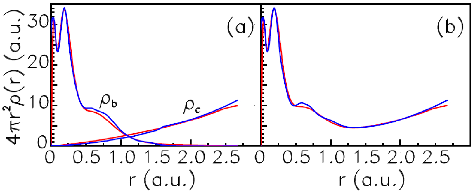
Our results were verified by comparing with calculations [34] for iron. The bound, continuum and total densities for the iron ion in plasmas with the normal density at k_βT = 100 eV are shown in Figure 10.

As is seen from Figure 10, our results (red curves) are very close to the results from [34] (blue curves). The slight differences occur in ρ_b in ranges of maxima and minima where electron wave functions are usually very sensitive to all details of calculations and in ρ_c near the very WS boundary.

Next, we compare our final results for the iron ion with calculations [34]. Presented in

Table 6. Spectrum of binding energies ε_i, level populations N_i, N_bound, the charge q and the chemical potential μ for the iron ion at k_βT = 100 eV and R_WS = 2.67 a.u.

Shell	Present Calculations				Calculations [34]
	DS–DS		DS–TF		DS–TF
	εi (eV)	Ni	εi (eV)	Ni	εi (eV)	Ni
1s	−7,110.47	2.0000	−7,110.04	2.0000	−7,109.00	2.0000
2s	−931.91	1.9986	−931.50	1.9986	−930.76	1.9988
2p1/2	−822.84	1.9957	−822.16	1.9957	−821.40	1.9964
2p3/2	−809.92	3.9903	−809.51	3.9903	−808.75	3.9919
3s	−170.02	0.8122	−169.77	0. 8147	−169.96	0.9087
3p1/2	−136.27	0.6559	−136.03	0. 6581	−136.19	0.7453
3p3/2	−134.12	1.2928	−133.88	1.2973	−134.04	1.4707
3d3/2	−80.38	0.8725	−80.08	0.8757	−80.14	1.0131
3d5/2	−80.06	1.3054	−79.76	1.3103	−79.81	1.5159
4s	−17.06	0.2580	−16.14	0.2577	−9.55	0.2868
Nbound		15.1814		15.1985		15.9277
q		10.8186		10.8015		10.0723
μ (eV)	−208.04		−207.27		−188.27

are the spectrum of binding energies ε_i, level populations N_i (Equation (29)), the chemical potential μ, the ion charge q and a number of bound electrons Nbound in the resulting ion:

$$N_{\text{bound}}={\displaystyle \sum _i{N}_i=Z-q}$$

(53)

Our data were obtained using the DS-TF and DS-DS models. One can see that the results calculated by the DS-TF model correlate with data from [34], where the same model has been adopted. Our binding energies are in excellent agreement with those from [34]. The largest difference for the binding energy of the valence 4s level is likely to be due to different boundary conditions. However, the difference in level occupation numbers reaches ∼12%. In addition, data of Table 6 allow one to compare results obtained within the DS-DS and DS-TF models. As is seen, there is a minor difference between the two calculations. The largest difference (∼5%) occurs for the binding energy of the valence 4s shell. Values of μ obtained in the two models differ by ≲0.3%, and values of the charge q only by ∼0.2%. It should be noted that all levels and the chemical potential become lower, as well as the charge increases when passing from the DS-TF model to the DS-DS one.

As is well known, the DS and TF continuum densities diverge drastically, the DS density ρ_c(r) being an oscillating function, while the TF ρ_c(r) is a quite smooth function. Nevertheless, the results obtained using the DS-DS and DS-TF models are very close to each other.

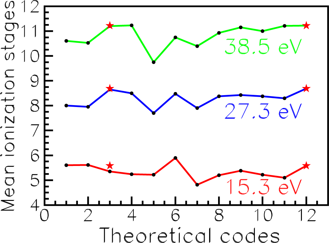
In addition, we compare our ion charge q for iron in three cases listed in

Table 7. Comparison of ionization stages q for Fe obtained in present calculations with mean ionization stages <q> from OP [38].

Case	kβT (eV)	ρ (mg/cm3)	q, Present	<q>, OP
1	15.3	5.48	5.58	5.35
2	27.3	3.39	8.69	8.65
3	38.5	2.63	11.22	11.2

with mean ionization stages < q > obtained by eight groups from Los Alamos, Livermore and with the data from Opacity Project (OPAC collaboration). The results have been calculated with different eleven codes to prepare LULI (Laboratoire pour L’Utilization des Lasers Intenses) 2010 experiments [37]. The difference in the mean ionization stage obviously implies the discrepancy between the frequency-dependent opacity. Therefore, the data are of importance for astrophysics.

As is shown in Figure 11, our values of q (red asterisks versus codes with numbers 12 and 3) correlate well with previous calculations. Besides, the data of Table 7 show that our results are in excellent agreement with the best results [37] of < q > from OP. The largest difference is 4%.

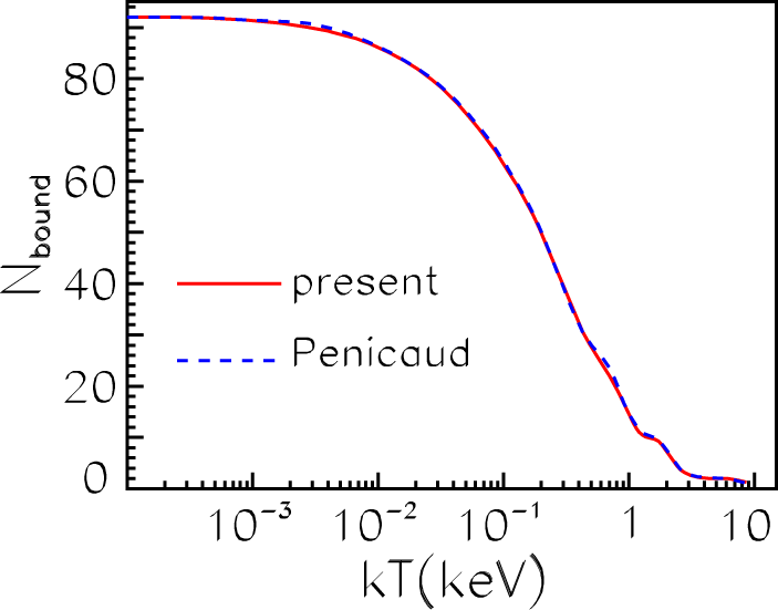
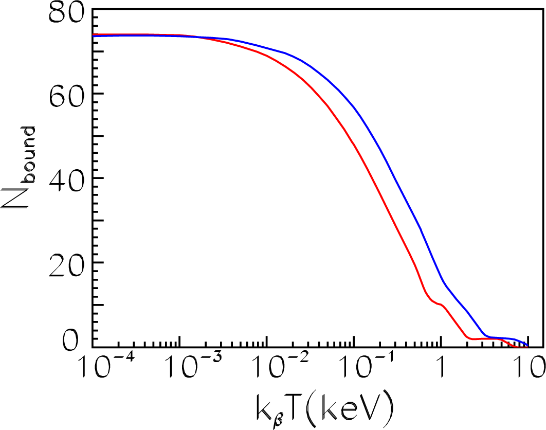
We also compared results for the heavy uranium ion with those obtained in [22] using code PARADISIO. In Figure 12, the number of bound electrons N_bound (Equation (53)) versus a temperature is presented for the uranium ion in plasmas with the density ρ = 0.01 g/cm³ (N_ion=2.5·10¹⁹ cm⁻³). As is seen, our calculation (red curve) is in excellent agreement with the previous results (blue dashed curve) in the wide temperature range 0.1 eV≤ k_βT ≤ 10 keV.

4.3. Results for Tungsten Ions

New calculations were performed within the DS-DS model for the tungsten ion in laser plasmas of two densities ρ₁ = 1.93 g/cm³ (the ion density N_ion = 6.3 × 10²¹cm⁻³) and ρ₂ = 0.01g/cm³ (N_ion = 3.3 × 10¹⁹cm⁻³). The spectrum of energies ε_i and level occupation numbers N_i are given in

Table 8. Spectrum of energies ε_i and level populations N_i for the tungsten ion in plasmas with densities ρ₁ = 1.93 g/cm³, R_WS = 6.339 a.u. and ρ₂ = 0.01 g/cm³, R_WS = 36.635 a.u.

ρ (g/cm3)	1.93				0.01
kβT (eV)	100		1000		100
Shell	εi (eV)	Ni	εi (eV)	Ni	εi (eV)	Ni
1s	−69,722.54	2.0000	−73,417.13	2.0000	−70,164.51	2.0000
2s	−12,372.45	2.0000	−15,833.79	1.9999	−12,814.53	2.0000
2p1/2	−11,855.50	2.0000	−15,375.08	1.9998	−12,297.85	2.0000
2p3/2	−10,501.65	4.0000	−13,987.02	3.9982	−10,943.37	4.0000
3s	−3,166.07	2.0000	−6,021.08	0.8729	−3,599.70	2.0000
3p1/2	−2,935.18	2.0000	−5,847.31	0.7885	−3,369.64	2.0000
3p3/2	−2,641.56	4.0000	−5,486.22	1.2483	−3,074.47	4.0000
3d3/2	−2,250.91	4.0000	−5,240.91	1.0478	−2,686.26	4.0000
3d5/2	−2,187.19	6.0000	−5,156.31	1.4756	−2,622.14	6.0000
4s	−943.61	1.9899	−2,992.50	0.0722	−1,341.97	1.9793
4p1/2	−846.60	1.9737	−2,917.45	0.0672	−1,244.62	1.9461
4p3/2	−771.68	3.8903	−2,777.18	0.1173	−1,164.57	3.7675
4d3/2	−611.08	3.5074	−2,675.58	0.1063	−1,003.80	3.0579
4d5/2	−596.36	5.1603	−2,641.73	0.1542	−987.58	4.4041
4f5/2	−393.86	2.6872	−2,559.40	0.1423	−788.06	1.6374
4f7/2	−390.46	3.5159	−2,545.99	0.1873	−784.05	2.1200
5s	−340.19	0.6434	−1,699.91	0.0204	−664.83	0.1973
5p1/2	−301.56	0.4875	−1,661.98	0.0196	−622.67	0.1340
5p3/2	−279.82	0.8237	−1,593.62	0.0367	−594.56	0.2057
5d3/2	−217.64	0.4890	−1,542.96	0.0349	−525.70	0.1060
5d5/2	−213.51	0.7072	−1,526.14	0.0514	−519.92	0.1503
5f5/2	−141.06	0.3649	−1,485.69	0.0494	−438.97	0.0678
5f7/2	−140.15	0.4824	−1,478.91	0.0654	−437.49	0.0891
5g7/2	−81.19	0.2749	−1,453.32	0.0638	−372.22	0.0467
5g9/2	−81.09	0.3432	−1,449.76	0.0795	−371.92	0.0582
6s	−138.52	0.1188	−1,033.83	0.0105	−393.88	0.0145
6p1/2	−121.22	0.1008	−1,012.24	0.0103	−372.63	0.0117
6p3/2	−112.55	0.1857	−974.08	0.0198	−359.21	0.0205
6d3/2	−84.58	0.1420	−945.29	0.0193	−324.12	0.0145
6d5/2	−82.89	0.2096	−935.78	0.0286	−321.26	0.0211
6f5/2	−50.56	0.1531	−912.78	0.0280	−280.20	0.0140
6f7/2	−50.17	0.2034	−908.90	0.0371	−279.43	0.0185
7s	−52.94	0.0522	−647.85	0.0072	−256.64	0.0037
7p1/2	−44.39	0.0481	−634.47	0.0071	−244.52	0.0033
7p3/2	−40.42	0.0925	−611.16	0.0138	−237.03	0.0061
7d3/2	−26.66	0.0808	−593.27	0.0136	−216.78	0.0050
7d5/2	−25.89	0.1203	−587.41	0.0202	−215.14	0.0073
Nbound		56.8484		16.9143		48.1074
q		17.1516		57.0857		25.8926
μ (eV)	−414.80		−6,276.71		−886.06

for the tungsten ion in plasmas with densities ρ₁ and the associated value of R_WS = 6.339 a.u. at temperatures 100 eV and 1,000 eV, as well as for ρ₂ and R_WS = 36.635 a.u. at temperature 100 eV. Comparing data for ρ₁ at different temperatures, it may be noted that the ion compresses when the plasmas temperature increases, i.e., the levels become deeper and the outer shell occupation numbers decrease. As is seen from comparison data for various densities at k_βT = 100 eV, the ion compresses when the plasmas density decreases. As is seen from Table 8, high electron states contribute significantly at the higher density and lower temperature. For example, the 5f, 5g, 6s, 6p, 6d, 6f and 7d levels have occupation numbers from ∼0.1–∼0.5 in the case of ρ₁ and k_βT = 100 eV. Occupation numbers for all levels decrease with the temperature increasing and the density decreasing.

The temperature dependence of N_bound is presented in Figure 13 for the two densities. The blue curve refers to ρ₁ and the red curve to ρ₂. A comparison between the two curves gives an idea of the plasmas density dependence. As is seen, the red and blue curves are not too different, even though the associated densities differ by ∼200-times. Increasing of a plasmas density shifts the curve N_bound(kβT) to higher temperatures.

To study tungsten impurities in fusion plasmas, we use the non-linear SCF screening model [39,40] for the calculation of the screening impurity potential. In the model, impurities in plasmas are considered as neutral pseudo-atoms. R_WS is assumed to be large. The chemical potential μ is found before the SCF calculations on the basis of the prescribed values of the plasmas electron density N_e and temperature k_βT using the following expression [40]:

$$N_{\epsilon }=\frac{\sqrt{2}}{{\pi }^2}{(k\beta T)}^{3/2}{\displaystyle \underset{0}{\overset{\infty }{\int }}\frac{y^{1/2}dy}{1+\exp (y-\mu /k\beta T)}}$$

(54)

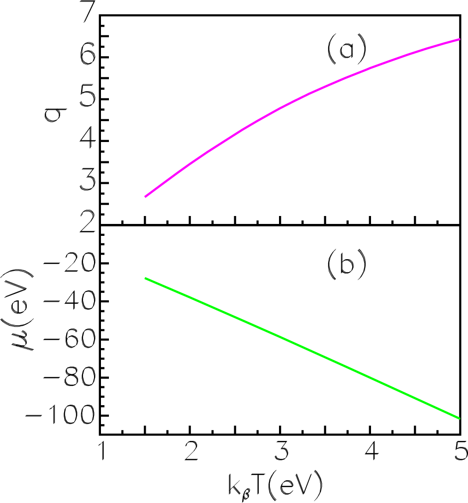
We consider the typical fusion plasmas density N_e = 10¹⁴cm⁻³ and the low temperature range 1 eV ≤ k_βT ≤ 5 eV. The SCF potential V (r) and the total electron density ρ(r) are found by the iterative process described above. The DS-DS model is used.

In Figure 14, the ion charge q (14a) and the chemical potential μ (14b) are displayed. As is evident, values of the charge and chemical potential change noticeably when the temperature increases. In

Table 9. Spectrum of energies ε_i and level populations N_i for the tungsten ion at low temperatures (k_βT = 2, 3 eV) as well as for a free neutral tungsten atom (k_βT = 0).

kβT (eV)	0.0		2.0		3.0
Shell	εi (eV)	Ni	εi (eV)	Ni	εi (eV)	Ni
1s	−69,312.37	2.0	−69,346.96	2.0000	−69,367.14	2.0000
2s	−11,956.28	2.0	−11,990.83	2.0000	−12,011.08	2.0000
2p1/2	−11,439.93	2.0	−11,474.51	2.0000	−11,494.76	2.0000
2p3/2	−10,088.80	4.0	−10,123.37	4.0000	−10,143.62	4.0000
3s	−2752.49	2.0	−2786.88	2.0000	−2806.91	2.0000
3p1/2	−2521.35	2.0	−2555.74	2.0000	−2575.79	2.0000
3p3/2	−2229.29	4.0	−2263.68	4.0000	−2283.70	4.0000
3d3/2	−1837.59	4.0	−1872.00	4.0000	−1892.07	4.0000
3d5/2	−1774.01	6.0	−1808.42	6.0000	−1828.49	6.0000
4s	−566.71	2.0	−601.09	2.0000	−621.06	2.0000
4p1/2	−470.77	2.0	−505.15	2.0000	−525.13	2.0000
4p3/2	−402.85	4.0	−437.23	4.0000	−457.21	4.0000
4d3/2	−244.71	4.0	−279.10	4.0000	−299.07	4.0000
4d5/2	−232.20	6.0	−266.58	6.0000	−286.56	6.0000
4f5/2	−34.17	6.0	−68.50	6.0000	−88.39	6.0000
4f7/2	−31.93	8.0	−66.26	8.0000	−86.13	7.9992
5s	−78.80	2.0	−112.82	2.0000	−132.23	2.0000
5p1/2	−50.29	2.0	−84.06	2.0000	−103.16	2.0000
5p3/2	−40.40	4.0	−73.90	4.0000	−92.67	4.0000
5d3/2	−5.10	4.0	−36.20	1.2052	−53.32	0.5788
5d5/2			−35.20	1.2392	−52.15	0.6149
6s	−6.35	2.0	−31.99	0.0996	−45.45	0.0242
6p1/2			−25.14	0.0034	−37.44	0.0017
6p3/2			−23.47	0.0030	−35.25	0.0016
Nbound		74.0		70.5504		69.2204
q		0.0		3.4496		4.7796
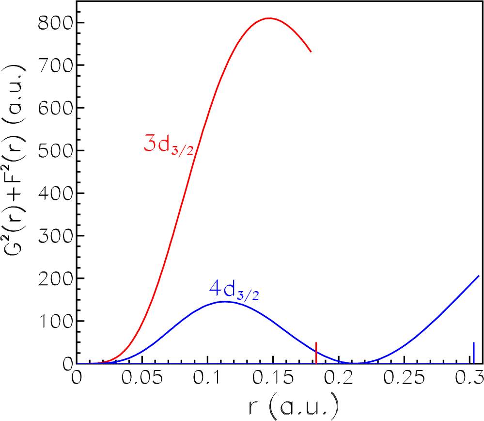
μ (eV)			−37.89		−58.66

, we present spectra obtained for the tungsten ion at various values of temperature. The case k_βT = 0 refers to the usual DS calculations for a free neutral tungsten atom. One can see that the increasing of temperature causes all binding energies of inner levels to become lower by approximately the same value. Outer levels also become lower, relatively to a greater extent. Consequently, the energy spectrum depends considerably on a plasma temperature, the changes being different for inner and outer levels. Calculations showed that only valence 5d_3/2 and 5d_5/2 states have large occupation numbers, while other excited states involved in calculations with regard to a temperature, for example 5f, 6d, 6f, 7d, 7s and 7p, have zero occupation numbers. The 6s and especially 6p states have very small occupation numbers (≲ 0:1), which decrease when temperature increases.

The data of Table 9 demonstrate different results for the free neutral atom (k_βT = 0) and for calculations with regard to a temperature. Nevertheless, this was just calculations for a free neutral atom, which were adopted as the initial data, as for instance in [41], where the non-LTE calculations in the collisional radiative model were performed. The average ionization stage < q > = 2.07 was obtained in [41] for the tungsten ion at the electron density Ne = 10¹⁴ cm⁻³ and k_βT = 2 eV. It was also shown that the largest contributions were made by transitions 5d³6s¹ → 5d³6p¹ and 5d⁴ → 5d³6p¹. This means that the 5d, 6s and 6p states are of primary importance in [41] as in our calculations. We obtained the ionization stage q = 3.45. Therefore, we believe that our results could be used as initial data in more sophisticated calculations rather than data for a free neutral atom. This may considerably change the results of these calculations.

5. Conclusions

• Our unified database on the RR and photoionization data was supplemented with partial and total RRCS and RR/RPL rates, as well as partial PCS for 54 tungsten ions from the range W⁶⁺–W⁷¹⁺. Fully relativistic calculations were performed by the DF method. All multipoles of a radiative field were taken into account. Total RRCS were calculated in the electron energy range from 1 eV–∼80 keV. Partial PCS were fitted in a wide photon energy range by the analytical expression with five fit parameters for all electron states with n ≤ 10 and ℓ ≤ 4. The fitting accuracy is usually better than 2%. Partial RRCS may be found by the use of the fit parameters and the relationship between RRCS and PCS. The partial and total RR/RPL rates were calculated in the temperature range from 10⁴ K–10⁹ K. Total RR rates were fitted by an analytical expression with four fit parameters. All results were added to the IAEA electronic database. The data are required for fusion studies, for example at the reactor ITER and devices ASDEX Upgrade and EBIT.
• The influence of the core electron polarization following the RR process on RRCS was investigated for the ion Fe XVII, as well as highly-charged tungsten ions. The inclusion of the PRR channel was shown to eliminate the puzzling discrepancy between experimental and theoretical values of EIECS for dominant X-ray lines from Fe XVII. It was found for highly-charged tungsten ions that the PRR enhancement factor may reach more than 15%. The factor depends on the photon energy, the principal quantum number of polarized shells and the ion charge. However, the factor is practically independent of the state into which an electron is captured in the RR process.
• The effect of plasmas temperature and density on the electron structure of an ion in LTE plasmas was studied. For this purpose, the code PLASMASATOM was created on the basis of the average-atom model. The bound and continuum electron densities are calculated by the relativistic DS method. Our calculations for the iron and uranium ions in dense plasmas are in good agreement with previous results. In particular, our calculations of the Fe ion charge q correlate well with the mean ionization stages <q> obtained by collaboration OPAC using various codes. Our values of q are in excellent agreement with the best data of <q> from the Opacity Project, the difference being in the range from 0.2%–4%.
• New calculations for the tungsten ion in dense plasmas demonstrated the temperature and dense dependence of the energy spectrum and level populations in a wide temperature range. Calculations were also performed for the impurity tungsten ion in fusion plasmas at low temperature. Comparison of the results with previous non-LTE calculations for tungsten impurity atoms allow one to arrive at the conclusion that our results could be used as initial data in more sophisticated calculations rather than data for a free neutral atom. This may change the results of these calculations.

References

1. Neu, R.; Dux, R.; Kallenbach, A.; Pütterich, T.; Balden, M.; Fuchs, J.C.; Herrmann, A.; Maggi, C.F.; O’Mullane, M.; Pugno, R.; et al. Tungsten: An option for divertor and main chamber plasma facing components in future fusion devices. Nucl. Fusion 2005, 45, 209–218. [Google Scholar]
2. Reader, J. Spectral data for fusion energy: From W to W. Phys. Scr 2009, 2009, 014023. [Google Scholar]
3. Skinner, C.H. Atomic physics in the quest for fusion energy and ITER. Phys. Scr 2009, 2009, 014022. [Google Scholar]
4. Biedermann, C.; Radtke, R.; Seidel, R.; Pütterich, T. Spectroscopy of highly charged tungsten ions relevant to fusion plasmas. Phys. Scr 2009, 2009, 014026. [Google Scholar]
5. Trzhaskovskaya, M.B.; Nikulin, V.K.; Clark, R.E.H. Radiative recombination and photoionization cross sections for heavy element impurities in plasmas. At. Data Nucl. Data Tables 2008, 94, 71–139. [Google Scholar]
6. Trzhaskovskaya, M.B.; Nikulin, V.K.; Clark, R.E.H. Radiative recombination rate coefficients for highly-charged tungsten ions. At. Data Nucl. Data Tables 2010, 96, 1–25. [Google Scholar]
7. Trzhaskovskaya, M.B.; Nikulin, V.K.; Clark, R.E.H. Horizons in World Physics; Reimer, A., Ed.; Nova: New York, NY, USA, 2012; Volume 277, Chapter 8; pp. 173–229. [Google Scholar]
8. Trzhaskovskaya, M.B.; Nikulin, V.K. Radiative recombination data for tungsten ions: I. W24+− W45+. At. Data Nucl. Data Tables 2013, 99, 249–311. [Google Scholar]
9. Trzhaskovskaya, M.B.; Nikulin, V.K. Radiative recombination data for tungsten ions: II. W47+− W71+. At. Data Nucl. Data Tables 2014, 100, 986–1058. [Google Scholar]
10. Trzhaskovskaya, M.B.; Nikulin, V.K. Radiative recombination data for tungsten ions: III. W 14+–W 23+. At. Data Nucl. Data Tables 2014, 100, 1156–1188. [Google Scholar]
11. Trzhaskovskaya, M.B.; Nikulin, V.K. Radiative Recombination and Photoionization Data of Heavy Element Impurities in Plasmas. Available online: http://www-amdis.iaea.org/DATASETS/a74.php accessed on 10 April 2015.
12. Nikulin, V.K.; Trzhaskovskaya, M.B. Comment on “Energy dependent excitation cross section measurements of diagnostic lines of Fe XVII”. Phys. Rev. Lett 2012, 108, 139301. [Google Scholar]
13. Brown, G.V.; Beiersdorfer, P.; Chen, H.; Scofield, J.H.; Boyce, K.R.; Kelley, R.L.; Kilbourne, C.A.; Porter, F.S.; Gu, M.F.; Kahn, S.M.; et al. Energy dependent excitation cross section measurements of diagnostic lines of Fe XVII. Phys. Rev. Lett 2006, 96, 253201. [Google Scholar]
14. Trzhaskovskaya, M.B.; Nikulin, V.K. Polarization Radiative Recombination Effect for Tungsten Highly-Charged Ions; Petersburg Nuclear Physics Institute Report No PNPI-2893; Petersburg Nuclear Physics Institute: Gatchina, Russia, 2012; pp. 1–22. [Google Scholar]
15. Trzhaskovskaya, M.B.; Nikulin, V.K. Atom in Dense Laser and Fusion Plasmas; Petersburg Nuclear Physics Institute Report No PNPI-2932; Petersburg Nuclear Physics Institute: Gatchina, Russia, 2013; pp. 1–26. [Google Scholar]
16. Band, I.M.; Listengarten, M.A.; Trzhaskovskaya, M.B.; Fomichev, V.I. Computer Program Complex RAINE. Part I; Leningrad Nuclear Physics Institute Report No LNPI-289; Leningrad Nuclear Physics Institute: Gatchina, Russia, 1976; pp. 1–54. [Google Scholar]
17. Band, I.M.; Trzhaskovskaya, M.B.; Fomichev, V.I. Computer Program Complex RAINE. Part III; Leningrad Nuclear Physics Institute Report No LNPI-299; Leningrad Nuclear Physics Institute: Gatchina, Russia, 1977; pp. 1–46. [Google Scholar]
18. Band, I.M.; Trzhaskovskaya, M.B.; Nestor, C.W., Jr.; Tikkanen, P.O.; Raman, S. Dirac–Fock internal conversion coefficients. At. Data Nucl. Data Tables 2002, 81, 1–334. [Google Scholar]
19. Liberman, D.A. Selfconsistent field for condensed matter. Phys. Rev. B 1979, 20, 4981–4989. [Google Scholar]
20. Bennet, B.I.; Liberman, D.A. Inferno; Los Alamos National Laboratory Report No LA-10309-M; Los Alamos National Laboratory: Los Alamos, NM, USA, 1985; pp. 1–32. [Google Scholar]
21. Wilson, B.; Sonnad, V.; Sterne, P.; Isaacs, W. Purgatorio—A new implementation of the Inferno algorithm. J. Quant. Spectrosc. Rad. Transfer 2006, 99, 658–685. [Google Scholar]
22. Pénicaud, M. An average atom code for warm matter: Application to aluminium and uranium. J. Phys 2009, 21, 095409. [Google Scholar]
23. Ichihara, A.; Eichler, J. Cross sections for radiative recombination and the photoelectric effect in the K, L, and M shells of one-electron systems with 1≤ Z ≤ 112 calculated within an exact relativistic description. At. Data Nucl. Data Tables 2000, 74, 1–121. [Google Scholar]
24. Alexanian, M. Photon bremsstrahlung from an extreme-relativistic electron gas. Phys. Rev 1968, 165, 253–257. [Google Scholar]
25. Trzhaskovskaya, M.B.; Nikulin, V.K.; Clark, R.E.H. Multipole and relativistic effects in radiative recombination process in hot plasmas. Phys. Rev. E 2008, 78, 035401(R). [Google Scholar]
26. Kramida, A.E.; Shirai, T. Energy levels and spectral lines of tungsten, W III through W LXXIV. At. Data Nucl. Data Tables 2009, 95, 305–474. [Google Scholar]
27. Verner, D.A.; Yakovlev, D.G.; Band, I.M.; Trzhaskovskaya, M.B. Subshell photoionization cross sections and ionization energies of atoms and ions from He to Zn. At. Data Nucl. Data Tables 1993, 55, 233–280. [Google Scholar]
28. Verner, D.A.; Ferland, G.J. Atomic data for astrophysics. I. Radiative recombination rates for H-like, He-like, Li-like, and Na-like ions over a broad range of temperature. Ap. J. Suppl 1996, 103, 467–473. [Google Scholar]
29. Astapenko, V.A.; Bureeva, L.A.; Lisitsa, V.S. Statistical models in polarization radiation theory Radiat. Phys. Chem 2006, 75, 1287–1307. [Google Scholar]
30. Badnell, N.R.; Pindzola, M.S. Unified dielectronic and radiative-recombination cross sections for U90+. Phys. Rev. A 1992, 45, 2820–2824. [Google Scholar]
31. Korol, A.V.; Gribakin, G.F.; Currell, F.J. The role of target polarization in electron-ion recombination. J. Phys. B 2004, 37, 2411–2428. [Google Scholar]
32. Korol, A.V.; Gribakin, G.F.; Currell, F.J. Effect of target polarization in electron-ion recombination. Phys. Rev. Lett 2006, 97, 223201. [Google Scholar]
33. Kogan, V.I.; Kukushkin, A.B.; Lisitsa, V.S. Kramers electrodynamics and electron-atomic radiative-collisional processes. Phys. Rep 1992, 213, 1–116. [Google Scholar]
34. Johnson, W.R. Photoabsorption in Hot Dense Plasmas. Available online: www3.nd.edu/∼johnson/Publications/tdlda/pdf accessed on 11 February 2001.
35. Johnson, W.R.; Guet, C.; Bertsch, G.F. Optical properties of plasma based on an average-atom model. J. Quant. Spectrosc. Rad. Transfer 2006, 99, 327–340. [Google Scholar]
36. Blenski, T.; Ishikawa, K. Pressure ionization in the spherical ion-cell model of dense plasmas and a pressure formula in the relativistic Pauli approximation. Phys. Rev. E 1995, 51, 4869–4881. [Google Scholar]
37. Gilles, D.; Turck-Chieze, S.; Loisel, G.; Piau, L.; Ducret, J.-E.; Poirier, M.; Blenski, T.; Thais, F.; Blancard, C.; Cossé, P.; et al. Comparison of Fe and Ni opacity calculations for a better understanding of pulsating stellar envelopes. High Energy Dens. Phys 2011, 7, 312–319. [Google Scholar]
38. Seaton, M.J.; Badnell, N.R. A comparison of Rosseland mean opacities from OP and OPAL. Mon. Not. R. Astron. Soc 2004, 354, 457–465. [Google Scholar]
39. Dharma-Wardana, M.W.C.; Perrot, F. Level shift continuum lowering and the mobility edge in dense plasmas. Phys. Rev. A 1991, 45, 5883–5896. [Google Scholar]
40. Perrot, F. Temperature-dependent nonlinear screening of a photon in an electron gas. Phys. Rev. A 1982, 25, 489–495. [Google Scholar]
41. Abdallah, J., Jr.; Colgan, J.; Clark, R.E.H.; Fontes, C.J.; Zhang, H.L.J. A collisional-radiative study of low-temperature tungsten plasma model. J. Phys. B 2011, 44, 075701. [Google Scholar]
Figure 1. The relativistic factor Frel for radiative recombination (RR) rates and radiated power loss (RPL) rates.
Atoms 03 00086f1
Figure 2. Partial RR cross-sections (RRCS) for RR of W6+ with an electron captured in the 5d3/2, 5f5/2 and 6p1/2 states. Red, Dirac–Fock (DF) calculation with regard to the exact electron exchange; blue, Dirac–Slater (DS) calculation with approximate consideration for the exchange.
Atoms 03 00086f2
Figure 3. Total RRCS (a), RR rates (b) and RPL rates (c) for representative tungsten ions. Rose, W6+; black solid, W14+; red, W17+; green, W20+; blue, W23+; yellow, W35+; light blue, W45+; black dashed W57+.
Atoms 03 00086f3
Figure 4. Partial RRCS (a), RR rates (b) and RPL rates (c) for the recombination of the W6+ ion with an electron captured in various states. Black, the 5d3/2; red, the 5f5/2; green, the 6s1/2; blue, the 6p1/2.
Atoms 03 00086f4
Figure 5. Feynman diagrams for amplitudes of the RR (a) and PRR (b) processes.
Atoms 03 00086f5
Figure 6. Enhancement factors F2 and F3 for the capture in the 4p state of the Ni-like ions. Red, present calculations; blue, exact non-relativistic calculations [31]. Vertical lines denote ionization energies obtained in the DF calculations. The lines relate from left to right to the 3d5/2 and 3d3/2 states merged together, the 3p3/2, 3p1/2, 3s and the 2p3/2, 2p1/2, 2s states.
Atoms 03 00086f6
Figure 7. The enhancement factor F2 for the capture in the 3s states of the Ne-like ions. Red, present calculations; blue, the exact non-relativistic calculations [31]. Vertical lines denote ionization energies of the 2p3/2, 2p1/2 and 2s states (from left to right) obtained by the DF method.
Atoms 03 00086f7
Figure 8. Enhancement factors Fn for RR of representative tungsten ions with an electron captured in the lowest state. Green, F4; blue, F3; rose, F2. Vertical lines denote ionization energies.
Atoms 03 00086f8
Figure 9. The electron density G2(r) + F 2(r) in the range [0 − r0] for the 3d3/2 (red) and 4d3/2 (blue) shells of the ion W28+. Vertical lines denote values of r0 for the 3d3/2 (red) and 4d3/2 (blue) shells.
Atoms 03 00086f9
Figure 10. The bound and continuum electron densities (a) and the total density (b) calculated using the DS-Thomas–Fermi (TF) model for the iron ion in laser plasmas at temperature kβT = 100 eV and the normal density 7.87 g/cm3, RWS = 2.67 a.u. Red, present calculations; blue, calculations [34].
Atoms 03 00086f10
Figure 11. Iron mean ionization stages < q > obtained by various codes. Codes used are: 1: FLYCHK (NLTE); 2: FLYCHK (LTE); 3: OP (·) and present results (*); 4: STA; 5: AA -ZP; 6: AA-ZM; 7: CASSANDRA; 8: OPAS; 9: SCO(rel.); 10: SCO-RCG; 11: LEDCOP; 12: present calculations (*), PLASMASATOM. Codes 5, 6 and 12 are LTE average atom ionization models. Figure is taken from [37] with our results added for comparison.
Atoms 03 00086f11
Figure 12. A number of bound electrons Nbound(kβT) for the uranium ion. Red solid, present calculations; blue dashed, results obtained in [22]. The plasma density is ρ = 0.01g/cm3.
Atoms 03 00086f12
Figure 13. A number of bound electrons Nbound(kβT) for the tungsten ion in plasmas of various densities. Blue, ρ1 = 1.93 g/cm3; red, ρ2 = 0.01 g/cm3.
Atoms 03 00086f13
Figure 14. The charge q (a) and the chemical potential μ (b) for the impurity tungsten ion in fusion plasmas.
Atoms 03 00086f14