The Second Workshop on Lineshape Code Comparison: Isolated Lines

 ,
,  ,
,  ,
, 

Abstract
:1. The Importance of Level Spacings
- Only a part of the collision duration is effective, i.e., the effective collision duration is shortened, not the entire collision.
- Since the impact parameter affects the collision duration (), the effective impact parameters are also smaller.
- The effective velocities increase (slow collisions are adiabatic).
- As a corollary to all the above, broadening is decreased.
2. Electron vs. Ion Broadening
3. Penetrating Collisions
4. Quantal Calculations
4.1. Work to be Done on Quantal Calculations
4.2. Work to be Done with Semiclassical Calculations
- The demarcation line between what may and what may not be treated semiclassically.
- Back-reaction issues, i.e., in classical terminology, deviations from the (straight line or hyperbolic) trajectory, due to the energy transfer between the perturber and emitter; e.g., for collisional excitation/deexcitation, in our case, between the 2s and 2p levels, given that these energy transfers are comparable to the thermal velocities.
5. (Dynamic) Shifts
6. The Codes
7. Strong Collisions
8. Calculational Uncertainties
- DARC. Calculation uncertainties were estimated by increasing the orbital angular momentum of the colliding electron up to 25. They turned out to be ≪5% [6].
- SimU. This is a full simulation code that computes the line profile directly instead of first computing the autocorrelation function. It is a semiclassical, long-range dipole code that handles non-perturbative aspects, as well as non-impact effects rigorously. SimU calculates , where is the dipole operator and is its Fourier transform. The procedure is repeated N times () and averaged, which corresponds to an averaging over a statistically representative ensemble of radiators. The uncertainty due to a finite statistical sampling is ∝, and the proportionality coefficient is inferred by observing convergence over the course of simulations. For details, see [26]. Another important factor affecting the calculational accuracy is the finite step of the frequency grid, equal to , where is the time over which is calculated in each run prior to averaging. Contrary to the first (statistical) factor, the latter always results in an overestimate of the line width by ∼. For the shift values, this factor contributes ±∼. The total uncertainties were within 10% for the cases considered.
- Simulation. The spectra is obtained through a Fourier transform of the autocorrelation function, which has been obtained by computer simulation and averaged over a large enough number of samples. The error is estimated using several sets of configurations to average the autocorrelation function and comparing the results obtained in each case. These fluctuations are about 3% using sets of 10,000 runs.
- Starcode. Starcode has two sources of errors: numerical errors, e.g., from integrations or solutions of the Schrödinger equation, which are controlled through appropriate tolerances and are generally negligible, and errors arising from the model used, which are the ones quoted here. Starcode recognizes that there is a part of the phase space for which the model used (e.g., semiclassical trajectories and, in the version without penetration, trajectories that penetrate the wavefunction extent) is not reliable. However, the contribution of that part of the phase space may be bound by unitarity. Thus, one first defines . This is a velocity below which all collisions have a de Broglie wavelength larger than the screening length, , and, hence, are definitely non-classical. The corresponding phase space makes a contribution:with n the electron density, the velocity distribution, and the S-matrices for the upper and lower levels, respectively, and α is an estimate for the average , which is between zero and two, due to unitarity. In practice, this contribution is negligible in our examples.For , the semiclassical approach is not valid for , where b is a parameter, taken to be one in the present calculations, which specifies how much larger than the de Broglie wavelength an impact parameter must be in order to be treatable semiclassically. Hence, if penetration is allowed, this non-semiclassical phase space provides the dominant contribution:If penetration is not allowed, then the upper limit of the ρ integral is with R the relevant wavefunction extent, e.g., the maximum spatial extent of the 2s and 2p levels in our case. Hence, in the case with penetration is replaced by with:with and andThis ensures that, provided one trusts the choices of b and R, only truly semiclassical paths are computed, and a rigorous, unitarity-based error bar may be returned for the part of the phase space that is not treatable semiclassically. Of course, other sources of error, e.g., the back reaction, are not accounted for.For the cases treated here with penetration not allowed, the wavefunction extent was dominant for all temperatures in the LiI calculations, for T = 15 and 50 eV for B III and T = 50 eV for NV. The de Broglie cutoff was dominant for the remaining cases. Hence, if the de Broglie cutoff is dominant, the Starcode and Starcode-NP calculations should have the same error bar, and Starcode-NP should have a larger width, due to the stronger interaction. If R is the dominant cutoff, then the error bar of Starcode-NP should be significantly larger and the computed width of Starcode might even exceed (with the error bar not accounted for) Starcode-NP, due to the larger phase space that is contributing. Of course, the situation will be reversed when the calculation uncertainties are accounted for. Width results are quoted as (the width from the part of phase space that is computed reliably error bar) error bar. Shifts are quoted as (the shift from the part of phase space that is computed reliably) ± error bar. All Starcode and Starcode-NP strong collision estimates assume a constant for that part of the phase space.
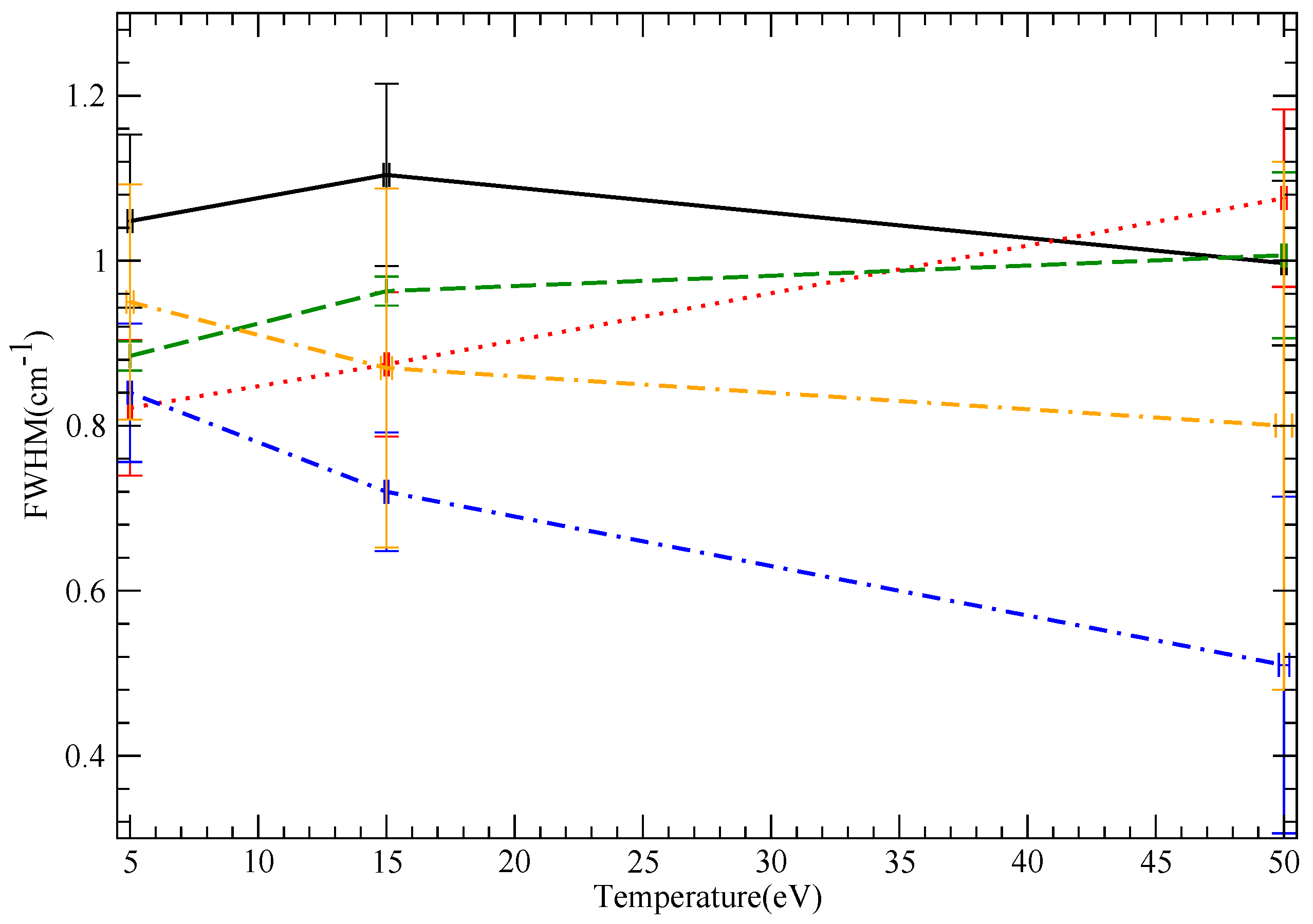
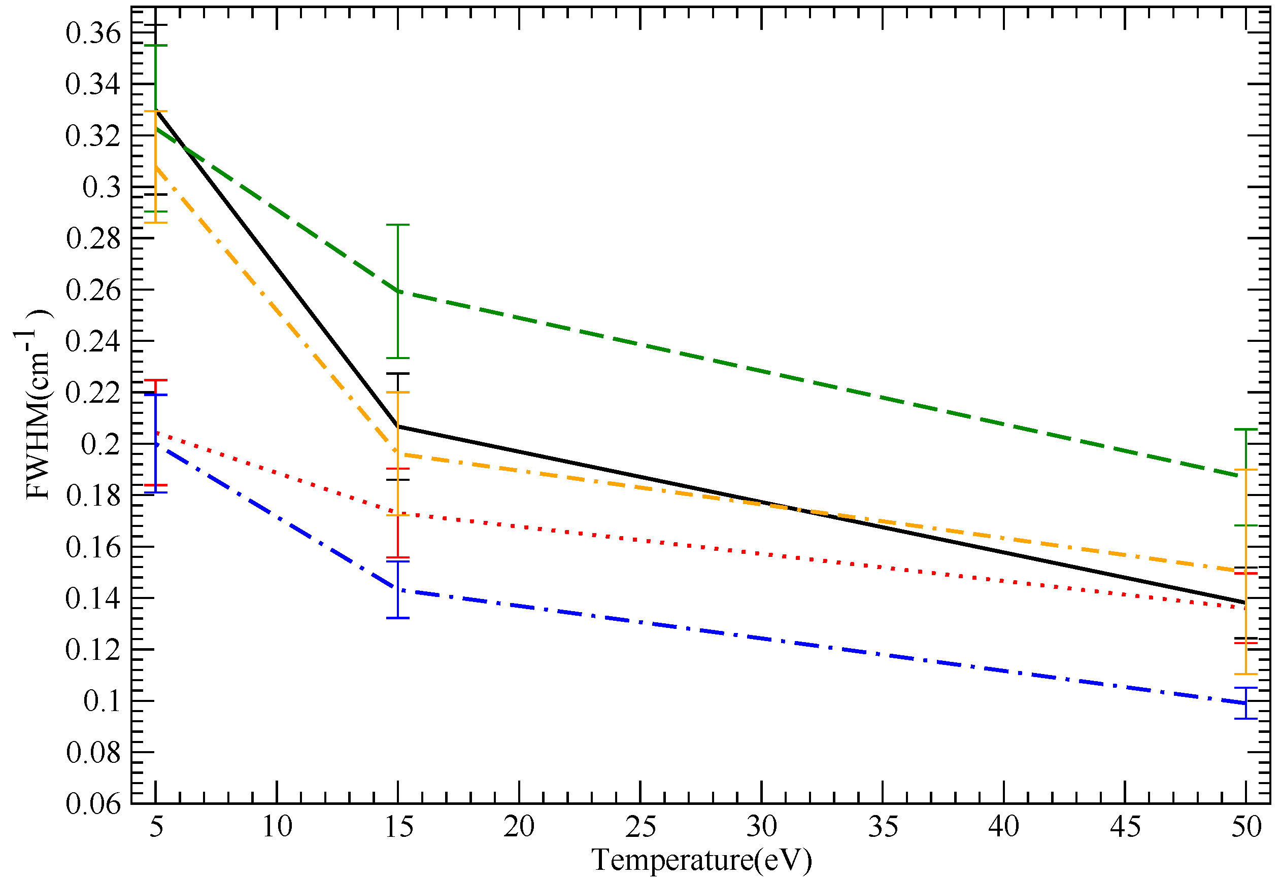
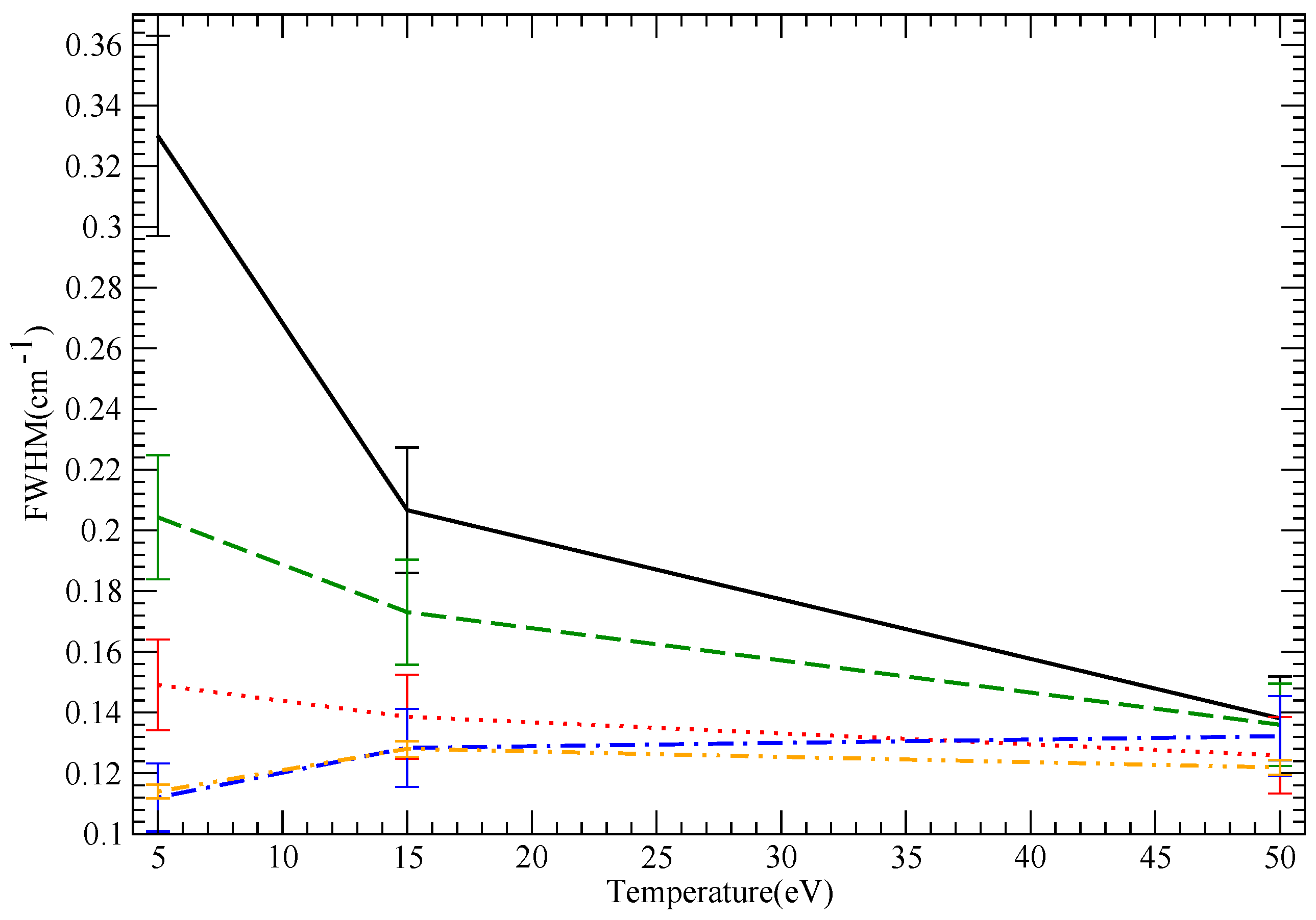
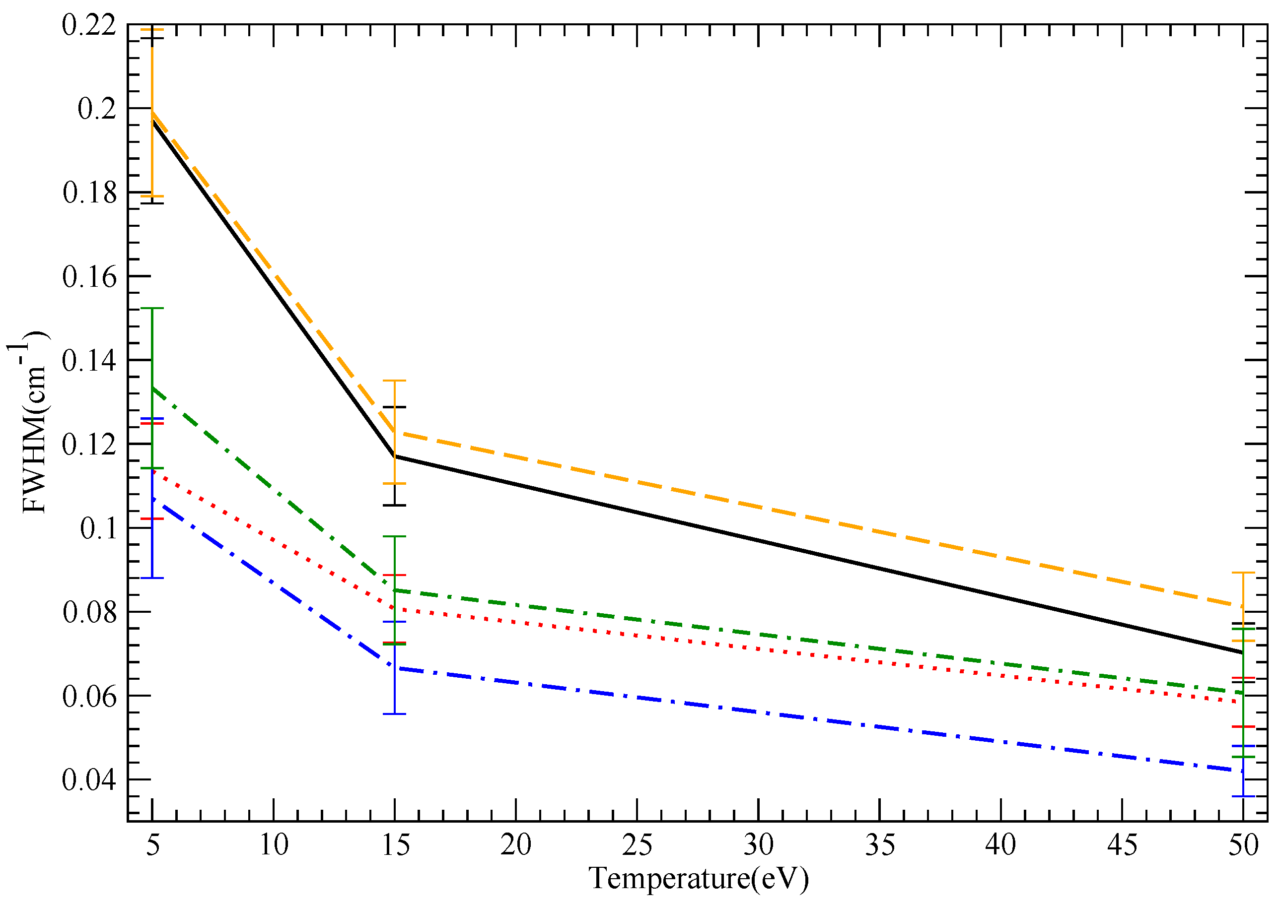
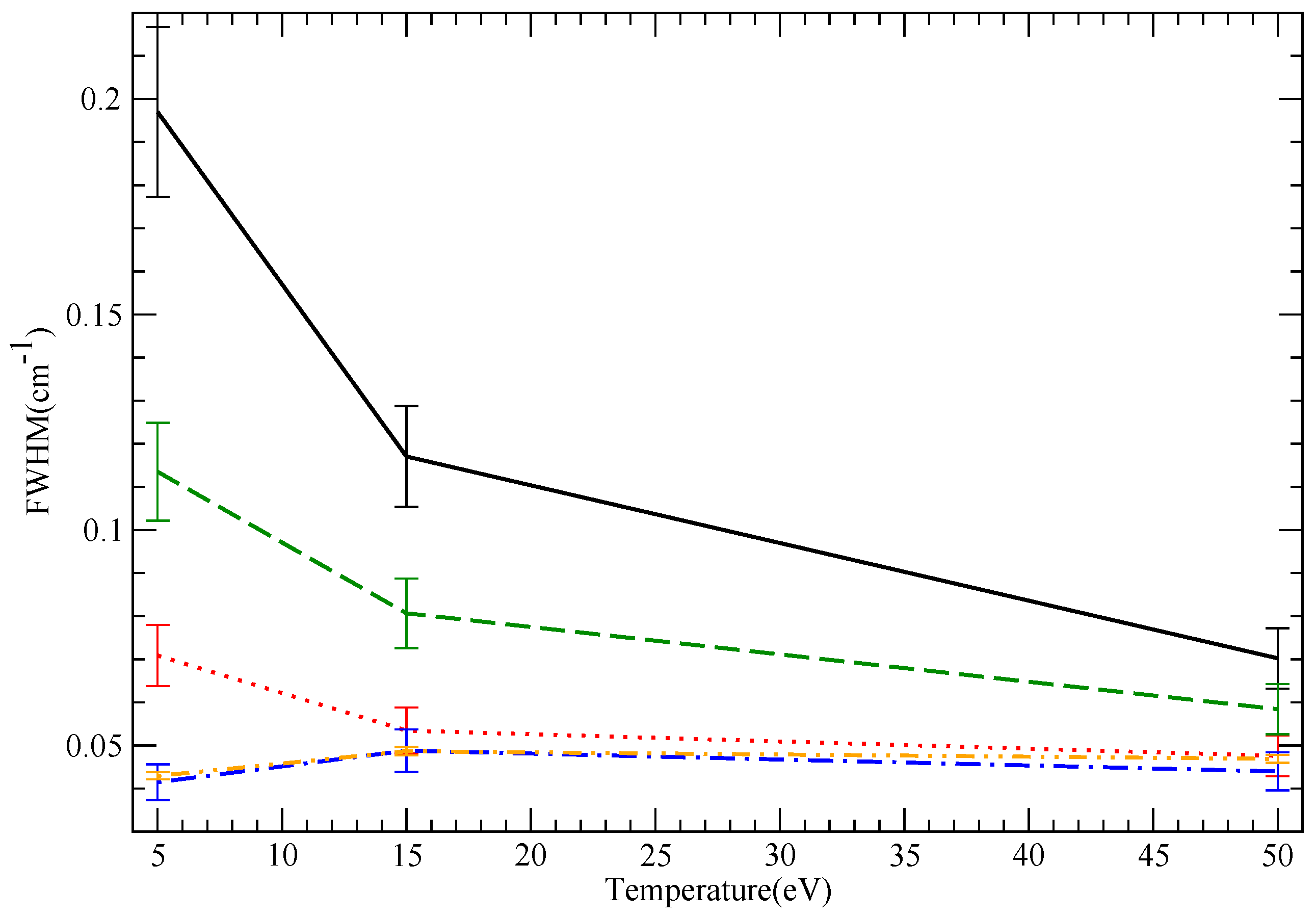
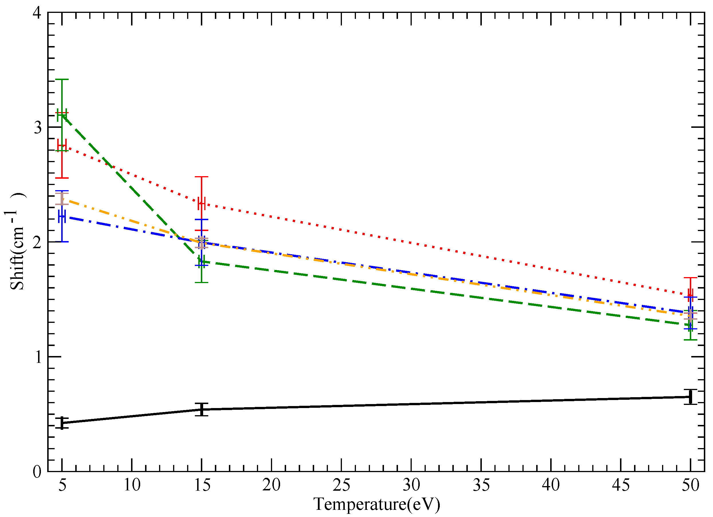
9. Results: Widths

| Species | T (eV) | Model | DARC | SCP | SimU | Simulation | Starcode-NP | Starcode |
|---|---|---|---|---|---|---|---|---|
| LiI | 5 | straight | 1.05 | 0.82 | 0.88 | 0.95 | 0.84 | |
| LiI | 15 | straight | 1.10 | 0.87 | 0.96 | 0.87 | 0.72 | |
| LiI | 50 | straight | 1.00 | 1.08 | 0.88 | 0.80 | 0.51 | |
| B III | 5 | hyperbolic | 0.322 | 0.33 | 0.2 | 0.3 | 0.2 | |
| B III | 5 | straight | 0.15 | 0.112 | 0.114 | |||
| B III | 15 | hyperbolic | 0.259 | 0.207 | 0.173 | 0.2 | 0.13 | |
| B III | 15 | straight | 0.139 | 0.128 | 0.128 | |||
| B III | 50 | hyperbolic | 0.187 | 0.138 | 0.136 | 0.15 | 0.092 | |
| B III | 50 | straight | 0.126 | 0.13 | 0.122 | |||
| NV | 5 | hyperbolic | 0.199 | 0.197 | 0.1135 | 0.133 | 0.088 | |
| NV | 5 | straight | 0.071 | 0.015 | 0.043 | |||
| NV | 15 | hyperbolic | 0.1228 | 0.117 | 0.08 | 0.084 | 0.056 | |
| NV | 15 | straight | 0.0535 | 0.0488 | 0.0487 | |||
| NV | 50 | hyperbolic | 0.0812 | 0.07 | 0.0584 | 0.06 | 0.036 | |
| NV | 50 | straight | 0.0476 | 0.044 | 0.0469 |
9.1. General Remarks
- In general, hyperbolic path calculations produced broader lines than straight line paths. This is expected, because due to the energy spacings (imaginary exponentials), only times closest to the time of the closest approach (t = 0) are important, but for these times, the electron is closer to the emitter if it is moving in a hyperbolic rather than a straight line path. Hence, the interaction is stronger, which results in larger widths.
- Non-perturbative collisions (impact or not) are treated correctly in simulations and by strong collision or error estimates in perturbative impact codes. This is not an issue for non-perturbative impact codes. Non-perturbative collisions are significant if penetration is not accounted for.
- Furthermore, in all cases, Starcode (with penetration) produces the lowest widths. This, however, is understood and expected, as Starcode with the option in question uses a different physical model that accounts for penetration, which, in turn, softens the interaction and results in smaller widths.
- DARC consistently produces large widths, in many cases, more than twice the results of Starcode, which also accounts for penetrating collisions. This is not understood and at variance with previous fully quantum mechanical close-coupling calculations, as discussed above.
- When investigating the differences between impact codes and simulations, particularly at low temperatures, one should keep in mind that impact codes treat all particles as impacting, while with simulation codes, the slow particles that are not impacting are treated correctly, i.e., differences could arise from non-impact effects for some particles. This would, in principle, mean lower widths for the simulations and should be less of an issue, at least for non-perturbative calculations at higher T. If that is correct, agreement should improve with non-perturbative impact calculations at higher T. As shown below, this is indeed the case for B III and NV, while the opposite is true for LiI. Note, however, that quantitatively non-impact effects are not expected to be an issue, as discussed below.
- Another issue is the temperature dependence, where we find some codes and cases with an increasing width with increasing temperature or a width that varies very little with temperature. Intuitively, one might expect that higher temperatures mean weaker collisions and, hence, smaller widths. We know, however, that an increase in temperature sometimes actually results in larger widths, e.g., for initially strong collisions, such as non-impact ions [27].Summing up, a non-decreasing temperature behavior, as observed in the simulation codes, may be the result of either non-impact effects or a significant or dominant strong collision term. The first possibility seems unlikely from simple estimates, discussed below, while if non-impact effects were negligible and the second were the case, then, since Starcode-NP is also a non-perturbative impact code, the differences from Starcode-NP would be due to the non-semiclassical phase space, as well as the emitter relevant wavefunction extent. This would have to be significant enough to change the widths vs. the temperature behavior. To check this conjecture, we list in Table 2 the Starcode-NP width contributions from the phase space part where Starcode-NP is presumably valid (labeled “non-strong” in Table 2, even though it includes non-perturbative collisions), as well as the “strong” collision contribution from the non-semiclassical and wavefunction extent phase space, where Starcode-NP (or any other workshop code, except DARC) is not valid. The actual width quoted is as described above, e.g., for the lowest LiI temperature.
| Species | T (eV) | Starcode-NP Non-Strong | Starcode-NP Strong |
|---|---|---|---|
| LiI | 5 | 0.83 | 0.23 |
| LiI | 15 | 0.69 | 0.39 |
| LiI | 50 | 0.48 | 0.7 |
| B III | 5 | 0.286 | 0.042 |
| B III | 15 | 0.172 | 0.048 |
| B III | 50 | 0.11 | 0.078 |
| NV | 5 | 0.114 | 0.038 |
| NV | 15 | 0.072 | 0.025 |
| NV | 50 | 0.0454 | 0.03 |
9.2. LiI Results
9.3. B III Results


9.4. NV Results


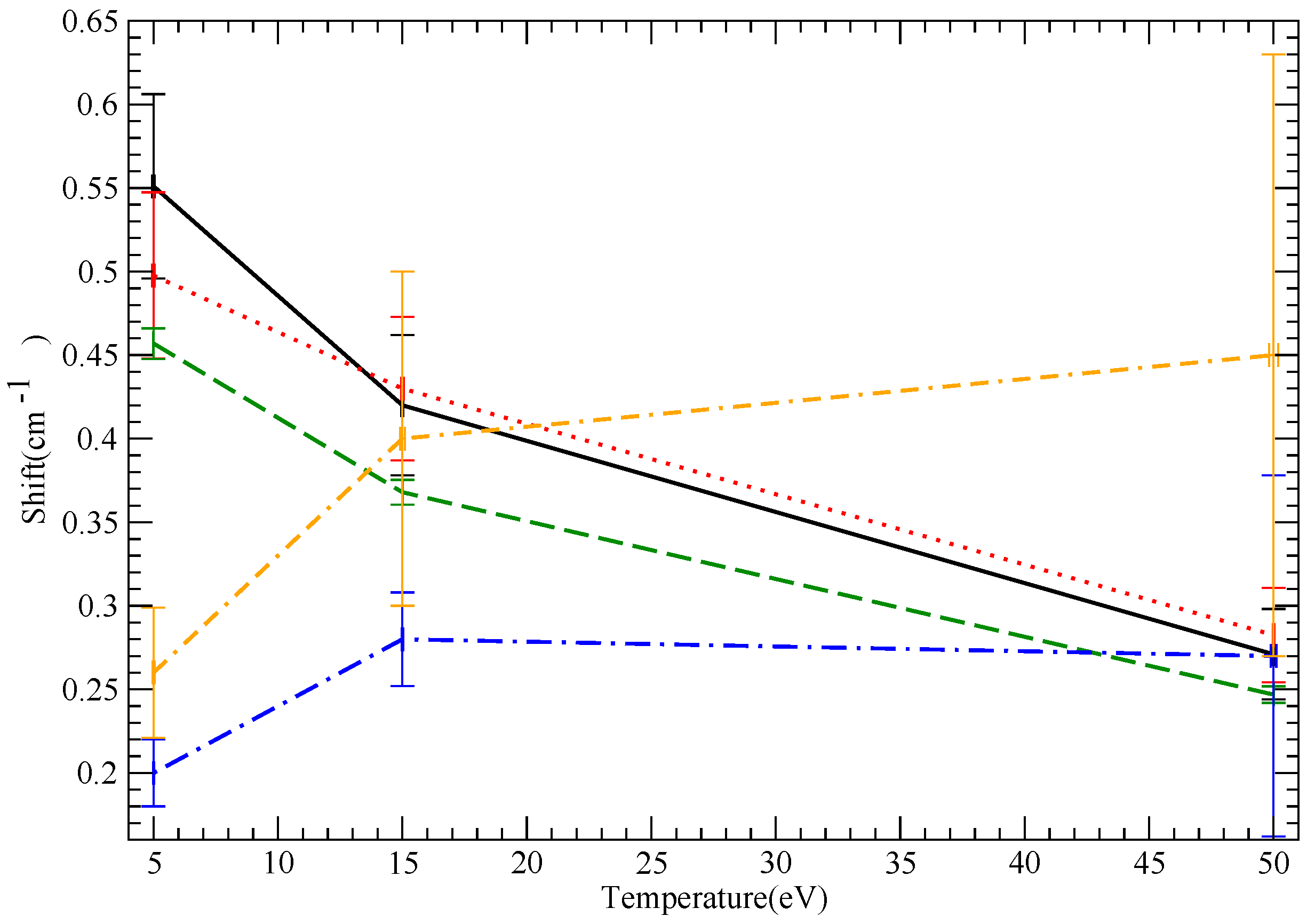
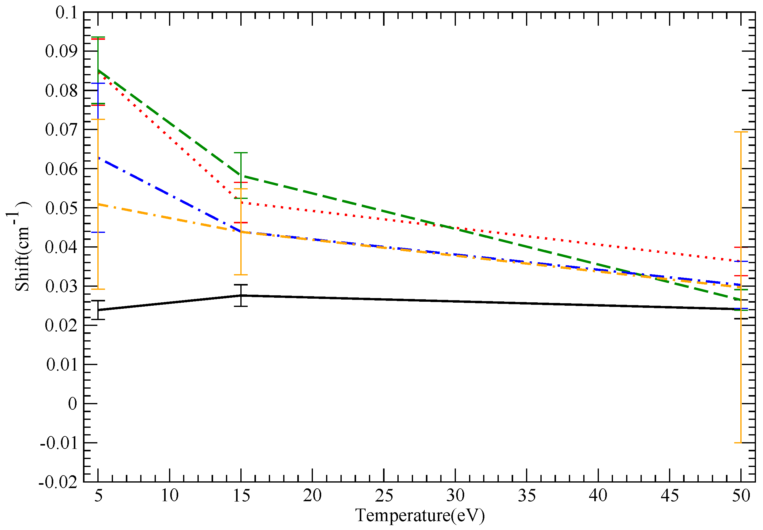
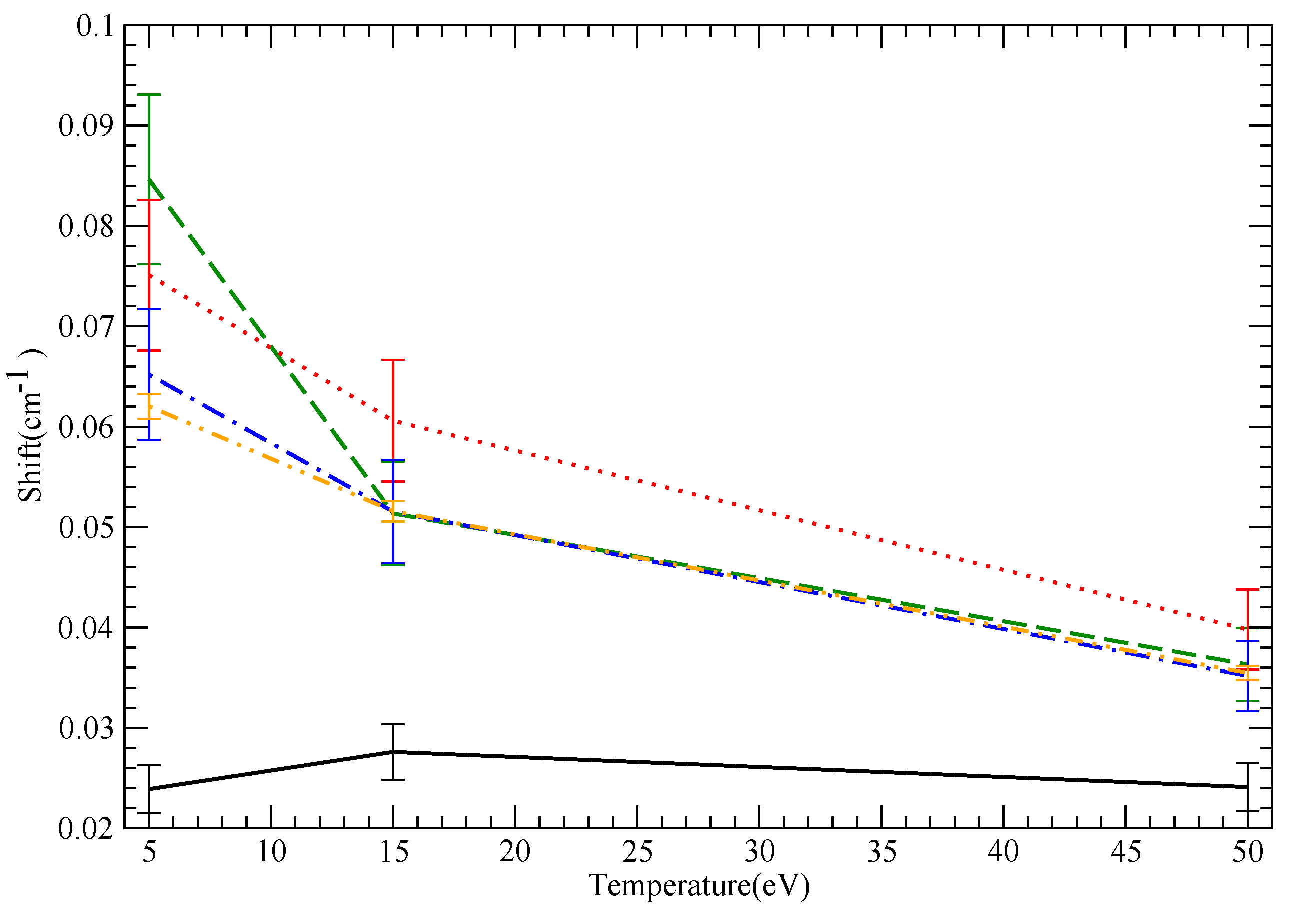
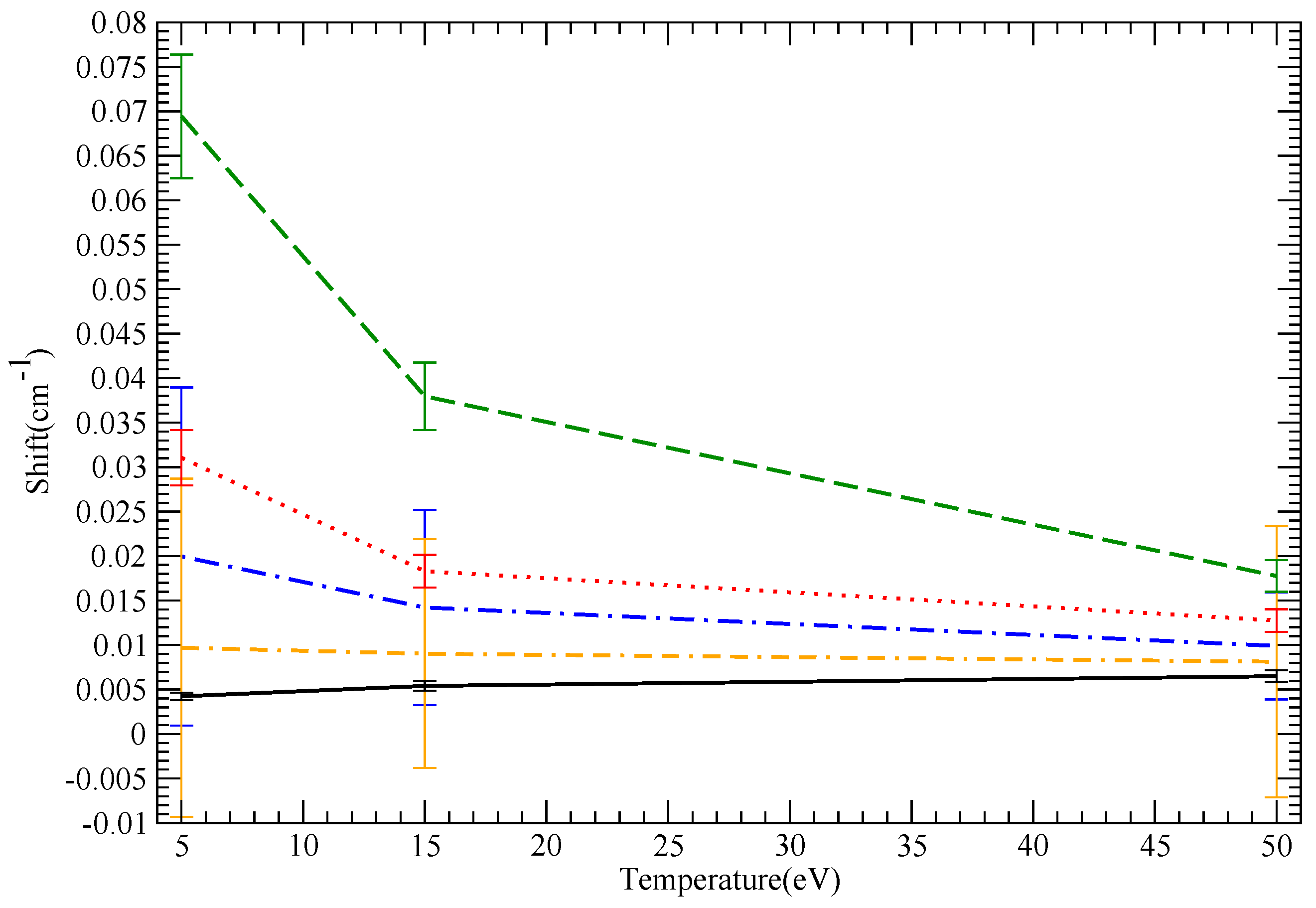
10. Results: Shifts
| Species | T (eV) | Model | DARC | SCP | SimU | Simulation | Starcode-NP | Starcode |
|---|---|---|---|---|---|---|---|---|
| LiI | 5 | straight | 0.551 | 0.498 | 0.457 | 0.21 | 0.2 | |
| LiI | 15 | straight | 0.42 | 0.43 | 0.368 | 0.29 | 0.28 | |
| LiI | 50 | straight | 0.271 | 0.282 | 0.247 | 0.29 | 0.27 | |
| B III | 5 | hyperbolic | 0.085 | 0.024 | 0.0846 | 0.05 | 0.063 | |
| B III | 5 | straight | 0.0751 | 0.065 | 0.062 | |||
| B III | 15 | hyperbolic | 0.058 | 0.0276 | 0.051 | 0.04 | 0.044 | |
| B III | 15 | straight | 0.0606 | 0.0515 | 0.0515 | |||
| B III | 50 | hyperbolic | 0.0265 | 0.0241 | 0.0363 | 0.03 | 0.03 | |
| B III | 50 | straight | 0.0398 | 0.0352 | 0.0355 | |||
| NV | 5 | hyperbolic | 0.0694 | 0.00423 | 0.031 | 1 | 2 | |
| NV | 5 | straight | 0.0284 | 0.0222 | 0.02375 | |||
| NV | 15 | hyperbolic | 0.03796 | 0.0054 | 0.0183 | 0.009 | 0.014 | |
| NV | 15 | straight | 0.0233 | 0.0199 | 0.0199 | |||
| NV | 50 | hyperbolic | 0.01776 | 0.0065 | 0.01275 | .008 | 0.01 | |
| NV | 50 | straight | 0.01535 | 0.0138 | 0.01355 |
10.1. General Remarks
- In general, we expect that if shifts are perturbative, they should also decrease with increasing T, due to the weakening of the interaction. For the same reason, we expect a convergence of the straight line and hyperbolic trajectory results as . No such statement of decreasing shifts with increasing T can be made with certainty in the non-perturbative case.
- Starcode, in particular (with or without penetration), often shows a very weak increase of shift with T, even in the version with penetration accounted for, which results in weak, perturbative collisions. The reason is that Starcode explicitly excludes the non-semiclassical phase space, e.g., impact parameters shorter than the de Broglie wavelength. (In addition, Starcode, without accounting for penetration, also excludes impact parameters inside the wavefunction extent, because, again, these may not be treated within a long-range approximation). When T decreases, this phase space, which may not be computed within the code’s semiclassical framework, increases. Hence, the phase space that gives a shift that may presumably be reliably computed shrinks, while the phase space that may not be treated grows. For both shifts and widths, Starcode binds the contribution of the non-semiclassical phase space by unitarity and returns it as an error bar. Therefore, while the quoted shift may be fairly insensitive to T, the error bar is not. These results are to be interpreted as an uncertainty in shift calculations inherent in semiclassical calculations, i.e., the part of the phase space that may not be treated semiclassically can make a substantial shift contribution rather than a temperature-insensitive shift.
- Straight line SimU and Simulation agreement is excellent for the charged cases (B III and NV), as expected and, surprisingly, much poorer (though still good) for LiI.
- SCP consistently gives significantly smaller shifts for ion lines (B III and NV). Furthermore, straight-line SCP calculations give significantly larger shifts than hyperbolic path SCP calculations. This is counterintuitive, since as discussed, hyperbolic paths result in a stronger effective interaction close to the emitter and, hence, action. Furthermore, the straight-line SCP shifts are monotonically decreasing as a function of T, in contrast to the hyperbolic trajectory results. This behavior follows the semiclassical b-functions [2], which result in lower shifts for hyperbolic compared to straight-line paths and, in addition, a decreasing b-function with increasing ion charge.
10.2. LiI

10.3. B III


10.4. NV
Acknowledgments
Author Contributions
Appendix A: Atomic Data
| Species | 2p Energy (cm) | Oscillator Strength |
|---|---|---|
| LiI | 14,903.89 | 0.7472 |
| B III | 48,381.07 | 0.3629 |
| NV | 80,635.67 | 0.234 |
Conflicts of Interest
References
- Griem, H.R. Plasma Spectroscopy; McGraw-Hill: New York, NY, USA, 1964. [Google Scholar]
- Griem, H.R. Spectral Line Broadening by Plasmas; Academic: New York, NY, USA, 1974. [Google Scholar]
- Alexiou, S. Collision operator for isolated ion lines in the standard Stark-broadening theory with applications to the Z scaling in the Li isoelectronic series 3P-3S transition. Phys. Rev. A 1994, 49, 106–119. [Google Scholar] [CrossRef] [PubMed]
- Elabidi, H.; Sahal-Brechot, S. Checking the dependence on the upper level ionization potential of electron impact widths using quantum calculations. Eur. Phys. J. D 2011, 61, 285–290. [Google Scholar] [CrossRef]
- Seidel, J. Effects of ion motion on hydrogen Stark profiles. Z. Naturforsch. 1977, 32a, 1207–1214. [Google Scholar] [CrossRef]
- Duan, B.; Bari, M.A.; Wu, Z.Q.; Jun, Y.; Li, Y.M. Widths and shifts of spectral lines in He II ions produced by electron impact. Phys. Rev. A 2012, 86, 052502. [Google Scholar] [CrossRef]
- Griem, H.; Ralchenko, Y.V.; Bray, I. Stark broadening of the B III 2s-2p lines. Phys. Rev. E 1997, 56, 7186–7192. [Google Scholar] [CrossRef]
- Alexiou, S.; Lee, R.W. Semiclassical calculations of line broadening in plasmas: Comparison with quantal results. J. Quant. Spectrosc. Radiat. Transf. 2006, 99, 10–20. [Google Scholar] [CrossRef]
- Alexiou, S. Phys. Rev. Lett. Problem with the standard semiclassical impact line-broadening theory. 1995, 75, 3406–3409.
- Alexiou, S.; ad Poque´russe, A. Standard line broadening impact theory for hydrogen including penetrating collisions. Phys. Rev. E 2005, 72, 046404. [Google Scholar] [CrossRef]
- Seaton, M.J. Line-profile parameters for 42 transitions in Li-like and Be-like ions. J. Phys. B 1988, 21, 3033–3054. [Google Scholar] [CrossRef]
- Ralchenko, Y.V.; Griem, H.; Bray, I.; Fursa, D.V. Electron collisional broadening of 2s3s-2s3p lines in Be-like ions. J. Quant. Spectrosc. Radiat. Transf. 2001, 71, 595–607. [Google Scholar] [CrossRef]
- Alexiou, S.; Lee, R.W.; Glenzer, S.; Castor, J. Analysis of discrepancies between quantal and semiclassical calculations of electron impact broadening in plasmas. J. Quant. Spectrosc. Radiat. Transf. 2000, 65, 15–22. [Google Scholar] [CrossRef]
- Elabidi, H.; Ben Nessib, N.; Cornille, M.; Dubau, J.; Sahal-Brechot, S. Electron impact broadening of spectral lines in Be-like ions: Quantum calculations. J. Phys. B 2008, 41, 025702. [Google Scholar] [CrossRef]
- Bouguettaia, H.; Chihi, Is.; Chenini, K.; Meftah, M.T.; Khelfaoui, F.; Stamm, R. Application of path integral formalism in spectral line broadening: Lyman-α in hydrogenic plasma. J. Quant. Spectrosc. Radiat. Transf. 2005, 94, 335–346. [Google Scholar] [CrossRef]
- Alexiou, S. Problems with the use of line shifts in plasmas. J. Quant. Spectrosc. Radiat. Transf. 2003, 81, 461–471. [Google Scholar] [CrossRef]
- Gunderson, M.A.; Haynes, D.A.; Kilcrease, D.P. Using semiclassical models for electron broadening and line shift calculations of Δn=0 and Δn≠0 dipole transitions. J. Quant. Spectrosc. Radiat. Transf. 2006, 99, 255–264. [Google Scholar] [CrossRef]
- Stambulchik, E.; Maron, Y. A study of ion-dynamics and correlation effects for spectral line broadening in plasma: K-shell lines. J. Quant. Spectrosc. Radiat. Transf. 2006, 99, 730–749. [Google Scholar] [CrossRef]
- Gigosos, M.A.; Cardenoso, V. New plasma diagnosis tables of hydrogen Stark broadening including ion dynamics. J. Phys. B: Atomic, Mol. Opt. Phys. 1996, 29, 4795–4838. [Google Scholar] [CrossRef]
- Sahal-Brechot, S. Impact theory of the broadening and shift of spectral lines due to electrons and ions in a plasma. Astron. Astrophys. 1969, 1, 91–123. [Google Scholar]
- Sahal-Brechot, S. Impact theory of the broadening and shift of spectral lines due to electrons and ions in a plasma. Astron. Astrophys. 1969, 2, 322–354. [Google Scholar]
- Sahal-Brechot, S. Stark broadening of isolated lines in the impact approximation. Astron. Astrophys. 1974, 319, 319–321. [Google Scholar]
- Fleurier, C.; Sahal-Brechot, S.; Chapelle, J. Stark profiles of some ion lines of alkaline earth elements. J. Quant. Spectrosc. Radiat. Transf. 1977, 17, 595–604. [Google Scholar] [CrossRef]
- Dimitrijević, M.S.; Sahal-Brechot, S. Comparison of measured and calculated Stark broadening parameters for neutral-helium. Phys. Rev. A 1985, 31, 316–320. [Google Scholar] [CrossRef] [PubMed]
- Elabidi, H.; Sahal-Brechot, S.; Ben Nessib, N. Quantum Stark broadening of 3s-3p spectral lines in Li-like ions; Z-scaling and comparison with semi-classical perturbation theory. Eur. Phys. J. D 2009, 54, 51–64. [Google Scholar] [CrossRef]
- Stambulchik, E.; Alexiou, S.; Griem, H.R.; Kepple, P.C. Stark broadening of high principal quantum number hydrogen Balmer lines in low-density laboratory plasmas. Phys. Rev. E 2007, 75, 016401. [Google Scholar] [CrossRef]
- Gigosos, M.A.; Gonzalez, M.A.; Konjevic, N. On the Stark broadening of Sr+ and Ba+ resonance lines in ultracold neutral plasmas. Eur. Phys. J. D 2006, 40, 57–63. [Google Scholar] [CrossRef]
- Hegerfeldt, G.C.; Kesting, V. Collision-time simulation technique for pressure-broadened spectral lines with applications to Ly-α. Phys. Rev. A 1988, 37, 1488–1496. [Google Scholar] [CrossRef] [PubMed]
© 2014 by the authors; licensee MDPI, Basel, Switzerland. This article is an open access article distributed under the terms and conditions of the Creative Commons Attribution license (http://creativecommons.org/licenses/by/3.0/).
Share and Cite
Alexiou, S.; Dimitrijević, M.S.; Sahal-Brechot, S.; Stambulchik, E.; Duan, B.; González-Herrero, D.; Gigosos, M.A. The Second Workshop on Lineshape Code Comparison: Isolated Lines. Atoms 2014, 2, 157-177. https://doi.org/10.3390/atoms2020157
Alexiou S, Dimitrijević MS, Sahal-Brechot S, Stambulchik E, Duan B, González-Herrero D, Gigosos MA. The Second Workshop on Lineshape Code Comparison: Isolated Lines. Atoms. 2014; 2(2):157-177. https://doi.org/10.3390/atoms2020157
Chicago/Turabian StyleAlexiou, Spiros, Milan S. Dimitrijević, Sylvie Sahal-Brechot, Evgeny Stambulchik, Bin Duan, Diego González-Herrero, and Marco A. Gigosos. 2014. "The Second Workshop on Lineshape Code Comparison: Isolated Lines" Atoms 2, no. 2: 157-177. https://doi.org/10.3390/atoms2020157
APA StyleAlexiou, S., Dimitrijević, M. S., Sahal-Brechot, S., Stambulchik, E., Duan, B., González-Herrero, D., & Gigosos, M. A. (2014). The Second Workshop on Lineshape Code Comparison: Isolated Lines. Atoms, 2(2), 157-177. https://doi.org/10.3390/atoms2020157