Electronic Structure Calculations with the Exact Pseudopotential and Interpolating Wavelet Basis

Abstract

Electronic structure calculations are mostly carried out with Coulomb potential singularity adapted basis sets such as STO or contracted GTO. With another basis or for heavy elements, the pseudopotentials may appear as a practical alternative. Here, we introduce the exact pseudopotential (EPP) to remove the Coulomb singularity and test it for orbitals of small atoms with the interpolating wavelet basis set. We apply EPP to the Galerkin method with a basis set consisting of Deslauriers–Dubuc scaling functions on the half-infinite real interval. We demonstrate the EPP–Galerkin method by computing the hydrogen atom 1s, 2s, and 2p orbitals and helium atom configurations $\mathrm{He}1{\mathrm{s}}^2$, $\mathrm{He}1\mathrm{s}2\mathrm{s}{}^1\mathrm{S}$, and $\mathrm{He}1\mathrm{s}2\mathrm{s}{}^3\mathrm{S}$. We compare the method to the ordinary interpolating wavelet Galerkin method (OIW–Galerkin), handling the singularity at the nucleus by excluding the scaling function located at the origin from the basis. We also compare the performance of our approach to that of finite-difference approach, which is another practical method for spherical atoms. We find the accuracy of the EPP–Galerkin method to be better than both of the above-mentioned methods.

1. Introduction

The Coulomb singularity in the hamiltonian may appear as a challenge in electronic structure calculations. Singularity-adapted Slater type-atomic orbitals (STO) basis is the usual solution to this, and Gaussian-type contracted basis functions (GTO) have turned out to be useful with sufficient accuracy. The latter one is more popular due to other practical advantages.

Pseudopotentials removing the singularity are another possible solution to this problem. In this case, the core electrons do not play an essential role in the problem at hand or valence electrons are expanded in plane waves, like with heavy elements or periodic crystalline systems. In those cases, the pseudopotentials typically replace the nuclei and a number of core electrons with their charge distribution, and possibly, some other core properties.

One-dimensional interpolating wavelets have been used for atomic computations, for example, in Ref. [1]. Fischer and Defranceschi [2] have also solved hydrogen-like atoms with wavelets. In Ref. [1], we used ordinary Deslauriers–Dubuc interpolating wavelets [3,4,5] defined on the whole real axis, so including the negative real axis in the computations. We handled the singularity at the origin by excluding the scaling function at the origin from the basis. We used the nonstandard operator form for the various operators needed in the computations. We computed the Schrödinger equation of hydrogenlike atoms (ions) and Hartree–Fock equations of some light many-electron atoms (helium, lithium, beryllium, neon, sodium, magnesium, and argon). In this article, we repeat similar computations for hydrogen and helium atoms, but using a different method to handle the singularity of the potential and only one resolution level. We handle the singularity by computing the Schrödinger and Hartree–Fock equations for a range of variables $r\in \left[a,\infty \right]$, which does not contain the origin. Here, r is the position coordinate. The range $r\in \left[0,a\right]$ is neglected for hydrogen, and for helium, its contribution to the Slater integrals is computed using the hydrogenic orbitals.

Arias [6] developed formalism for electronic structure calculations with interpolating wavelets so that matrix elements of the operators are computed as usual, and overlap matrices are used in the matrix form of the Schrödinger equation. On the other hand, we use the interpolating dual scaling functions and wavelets for the computation of matrix elements.

One-dimensional interpolating multiresolution analysis in space $C_{\mathrm{u}}\left(\mathbb{R}\right)$ consisting of uniformly continuous bounded functions in $\mathbb{R}$ was conducted in Ref. [4]. One-dimensional interpolating multiresolution analysis in space $C_0\left(\mathbb{R}\right)$ consisting of continuous functions in $\mathbb{R}$ and vanishing at infinity was constructed in [5]. Both of these constructions are based on Deslauriers–Dubuc functions [3]. Donoho [5] constructs wavelets on a finite real interval, too. We compute the eigenenergies of hydrogen atom 1s, 2s, and 2p orbitals and helium atom configurations $\mathrm{He}1{\mathrm{s}}^2$, $\mathrm{He}1\mathrm{s}2\mathrm{s}{}^1\mathrm{S}$, and $\mathrm{He}1\mathrm{s}2\mathrm{s}{}^3\mathrm{S}$ with the EPP method Exact Pseudopotential Method (EPP) using both the Galerkin method with interpolating wavelets and the finite difference method.

We denote the pointwise product of functions f and g by $f★g$. We use atomic units throughout this article ($e=m_e=\hslash =4\pi {\epsilon }_0=1$) and denote the atomic unit of energy by $\mathrm{Ha}$ (Hartree).

2. Interpolating Wavelets on Half-Infinite Interval

2.1. Interpolating Wavelets

Interpolating wavelets are a biorthogonal wavelet family. Since the dual scaling functions and dual wavelets of these functions are finite sums of Dirac delta functions, the matrix elements involving interpolating wavelets usually require evaluating some functions in a finite set of points. An interpolating wavelet family is defined by a mother scaling function $\phi$, mother wavelet $\psi$, and four finite filters $h_j$, $g_j$, ${\tilde{h}}_j$, and ${\tilde{g}}_j$ where $j=-m,\dots ,m$. The functions $\phi$, $\psi$, $\tilde{\phi }$, and $\tilde{\psi }$ satisfy equations

$$\phi \left(x\right)=\sum _{j=-m}^m{h}_j\phi (2x-j),$$

(1)

$$\psi \left(x\right)=\sum _{j=-m}^m{g}_j\phi (2x-j),$$

(2)

$$\tilde{\phi }\left(x\right)=\sum _{j=-m}^m{\tilde{h}}_j\tilde{\phi }(2x-j),$$

(3)

and

$$\tilde{\psi }\left(x\right)=\sum _{j=-m}^m{\tilde{g}}_j\tilde{\phi }(2x-j).$$

(4)

The two-index basis functions and dual basis functions are

$${\phi }_{j,k}\left(x\right)=\phi (2^{j}x-k),$$

(5)

$${\psi }_{j,k}\left(x\right)=\psi (2^{j}x-k),$$

(6)

$${\tilde{\phi }}_{j,k}\left(x\right)=2^j\tilde{\phi }(2^{j}x-k),$$

(7)

and

$${\tilde{\psi }}_{j,k}\left(x\right)=2^j\tilde{\psi }(2^{j}x-k).$$

(8)

A wavelet basis consists of scaling functions ${\phi }_{j_0,k}$, $k\in \mathbb{Z}$, and wavelets ${\psi }_{j,k}$, $j\ge j_0$, $k\in \mathbb{Z}$, where $j_0\in \mathbb{Z}$ is the minimum resolution level. The expansion of an arbitrary (regular enough) function $f:\mathbb{R}\to \mathbb{R}$ in the wavelet basis is

$$f\left(x\right)=\sum _{k\in \mathbb{Z}}{s}_k{\phi }_{j_0,k}\left(x\right)+\sum _{j\ge j_0}\sum _{k\in \mathbb{Z}}{d}_{j,k}{\psi }_{j,k}\left(x\right).$$

(9)

2.2. The Basis Set

This derivation is based on Section 3 in [5]. We construct a basis set on half-infinite interval ${\mathbb{R}}_0=\{r\ge 0|r\in \mathbb{R}\}$. We define $\phi$ to be a Deslauriers–Dubuc scaling function of some order D and ${\phi }_{j,k}\left(x\right):=\phi (2^{j}x-k)$ for $j,k\in \mathbb{Z}$.

Suppose that we are given samples ${\beta }_{j,k}=f\left(2^{-j}k\right)$ for $k\in \mathbb{N}$ and f is some function from $[0,\infty ]$ into $\mathbb{R}$. We define ${\pi }_j^{\#}$ to be the polynomial of degree D for which ${\pi }_j^{\#}\left(2^{-j}k\right)=f\left(2^{-j}k\right)$ for all $k=0,\dots ,D$. We define

$${\tilde{\beta }}_{j,k}:={\pi }_j^{\#}\left(2^{-j}k\right)$$

(10)

for $k<0$ and

$${\tilde{\beta }}_{j,k}:={\beta }_{j,k}$$

(11)

for $k\ge 0$. Now, f can be extrapolated onto the whole real line by

$$\tilde{f}=\sum _{k=-\infty }^{\infty }{\tilde{\beta }}_{j,k}{\phi }_{j,k}.$$

(12)

As each coefficient ${\tilde{\beta }}_{j,k}$ is a linear functional of coefficients ${\beta }_{j,k^{\prime }}$, we may define extrapolation weights $e_{k,k^{\prime }}^{\#}$ so that

$${\tilde{\beta }}_{j,k}=\sum _{k^{\prime }=0}^D{e}_{k,k^{\prime }}^{\#}{\beta }_{j,k^{\prime }}$$

(13)

for $k<0$. When $f:={\phi }_{j,l}$, we have

$${\tilde{\beta }}_{j,k}=e_{k,l}^{\#}$$

(14)

where $l\in \{0,\dots ,D\}$. Consequently, the quantities $e_{k,l}^{\#}$ can be computed by polynomial interpolation of functions ${\phi }_{j,l}$. As

$$supp{\phi }_{j,k}\subset 2^{-j}[k-D,k+D]$$

(15)

we need only values $k\in \{-D,\dots ,-1\}$. We define

$${\phi }_{j,k}^{\#}:={\phi }_{j,k}+\sum _{l<0}{e}_{l,k}^{\#}{\phi }_{j,l}$$

(16)

for $k=0,\dots ,D$. Note that

$$⟨{\tilde{\phi }}_{j,k},{\phi }_{j,l}^{\#}⟩={\delta }_{k,l}$$

(17)

for $k\ge 0$ and $0\le l\le D$.

We define a wavelet expansion of function f by

$$\tilde{f}:=\sum _{k=0}^D{\beta }_{j,k}{\phi }_{j,k}^{\#}+\sum _{k=D+1}^{\infty }{\beta }_{j,k}{\phi }_{j,k}.$$

(18)

When we use a finite basis of size W, we have

$$\tilde{f}:=\sum _{k=0}^D{\beta }_{j,k}{\phi }_{j,k}^{\#}+\sum _{k=D+1}^{W-1}{\beta }_{j,k}{\phi }_{j,k}.$$

(19)

We must have $W>2D$ so that functions ${\phi }_{j,k}^{\#}\left(x\right)$, $0\le k\le D$, vanish for $x\ge 2^{-j}W$. This kind of truncation of the basis requires that the function f approximately vanishes for $x>2^{-j}W$.

Let A be a linear operator from $C_0\left(\mathbb{R}\right)$ to $C_0\left(\mathbb{R}\right)$. The matrix elements $A_{k,l}$, $l=0,\dots ,D$ are given by

$$⟨{\tilde{\phi }}_{j,k},A{\phi }_{j,l}^{\#}⟩=⟨{\tilde{\phi }}_{j,k},A{\phi }_{j,l}⟩+\sum _{\alpha <0}{e}_{\alpha ,l}^{\#}⟨{\tilde{\phi }}_{j,k},A{\phi }_{j,\alpha }⟩.$$

(20)

Let $v\left(f\right)$ denote the coefficient vector ${\left({\beta }_{j,k}\right)}_{k=0}^{W-1}$ defined by Equation (19) and define

$$M\left(f\right):={\left(f\left(2^{-j}k\right){\delta }_{k,k^{\prime }}\right)}_{k,k^{\prime }=0}^{W-1,W-1}$$

(21)

for some function $f:\mathbb{R}\to \mathbb{R}$.

3. Schrödinger Equations of Hydrogen-like Atoms and Helium Atoms in the EPP-Wavelet Basis

3.1. General

Suppose that we have a system consisting of a positively charged nucleus at the origin and N electrons. In the EPP method, we choose a small radius $r_0$ so that inside the sphere with radius $r_0$, the wavefunctions of the system are approximated by hydrogenic wavefunctions, and the actual computations are performed only for values $r\ge r_0$. Actually, we define a basis set for the half-infinite interval $\left[0,\infty \right]$ and make a change of the variables $s=r-r_0$. For Hartree–Fock calculations, the Slater integrals are computed by

$$\begin{array}{ccc}\hfill {\overline{y}}_{\mathrm{ab}}^0\left(s\right)& =& \frac{Q_{\mathrm{ab}}}{s+r_0}+\frac{1}{s+r_0}{\int }_0^s{\overline{P}}_{\mathrm{a}}\left(s^{\prime }\right){\overline{P}}_{\mathrm{b}}\left(s^{\prime }\right)d{s}^{\prime }\hfill \\ & & +{\int }_s^{\infty }\frac{1}{s^{\prime }+r_0}{\overline{P}}_{\mathrm{a}}\left(s^{\prime }\right){\overline{P}}_{\mathrm{b}}\left(s^{\prime }\right)d{s}^{\prime }\hfill \end{array}$$

(22)

where $s\ge 0$ and $Q_{\mathrm{ab}}$ is a system-dependent quantity that approximates the contribution of the EPP core region to the Slater integral.

3.2. Hydrogen-like Atoms

The Schrödinger equation of the hydrogen atom and Hartree–Fock equations of atoms [7] and their representation in the interpolating wavelet basis [1] denote our starting point. With a change in variables $s:=r-r_0$, the Schrödinger equation of a hydrogen-like atom in interval $r\ge r_0$ takes the form

$$\left(-\frac{1}{2}\frac{d^2}{d{s}^2}-\frac{Z}{s+r_0}+\frac{l(l+1)}{2^{(}s+r_0{)}^2}\right)\overline{P}\left(s\right)=E\overline{P}\left(s\right),s\ge 0$$

(23)

where Z is the charge of the nucleus, l is the angular momentum quantum number, and $\overline{P}\left(s\right)=P(r_0+s)$ for $s\ge 0$.

We define the second derivative filter by

$$a_k:=⟨\tilde{\phi },D^2\phi (·-k)⟩.$$

(24)

Matrix elements of the Laplacian operator L are computed by

$$L_{k,l}:=⟨{\tilde{\phi }}_{j,k},L{\phi }_{j,l}^{\#}⟩=2^{2j}\left(a_{l-k}+\sum _{\alpha =-D}^{-1}{e}_{\alpha ,l}^{\#}{a}_{\alpha -k}\right)$$

(25)

for $0\le l\le D$ and

$$L_{k,l}:=⟨{\tilde{\phi }}_{j,k},L{\phi }_{j,l}⟩=2^{2j}{a}_{l-k}$$

(26)

for $D<l<W$. Note that matrix L is generally not hermitian. The potential energy operator is computed as a diagonal matrix

$${\widehat{V}}_{k,k}=V\left(2^{-j}k\right)$$

(27)

where

$$V\left(y\right)=-\frac{Z}{y+a}$$

(28)

for $y\ge 0$. The centrifugal potential is computed in the same way.

3.3. Hartree–Fock Equations for Helium Atom

Define the Slater integrals as

$$y_{\mathrm{ab}}^0\left(r\right)={\int }_{r^{\prime }=0}^{\infty }{P}_{\mathrm{a}}\left(r^{\prime }\right)\gamma (r,r^{\prime })P_{\mathrm{b}}\left(r^{\prime }\right)d{r}^{\prime }$$

(29)

where a and b denote the atomic orbitals and

$$\gamma (r,r^{\prime })=\frac{1}{max\{r,r^{\prime }\}}.$$

(30)

We use symbol y instead of Y to avoid confusion with spherical harmonics. By carrying out a similar change in variables $s:=r-r_0$, the Hartree–Fock equation of the ground state of the helium atom in interval $r\ge r_0$ takes the form

$$\left(-\frac{1}{2}\frac{d^2}{d{s}^2}-\frac{2}{s+r_0}+y_{1\mathrm{s}1\mathrm{s}}^0(s+r_0)\right){\overline{P}}_{1\mathrm{s}}\left(s\right)={\epsilon }_{1\mathrm{s}}{\overline{P}}_{1\mathrm{s}}\left(s\right),s\ge 0.$$

(31)

The Hartree–Fock equations for the helium 1s2s ${}^1\mathrm{S}$ configuration are

$$\begin{array}{c}\hfill \left(-\frac{1}{2}\frac{d^2}{d{s}^2}-\frac{2}{s+r_0}+y_{2\mathrm{s}2\mathrm{s}}^0(s+r_0)\right){\overline{P}}_{1\mathrm{s}}\left(s\right)={\epsilon }_{1\mathrm{s}}{\overline{P}}_{1\mathrm{s}}\left(s\right)\end{array}$$

(32)

$$\begin{array}{c}\hfill \left(-\frac{1}{2}\frac{d^2}{d{s}^2}-\frac{2}{s+r_0}+y_{1\mathrm{s}1\mathrm{s}}^0(s+r_0)\right){\overline{P}}_{2\mathrm{s}}\left(s\right)={\epsilon }_{2\mathrm{s}}{\overline{P}}_{2\mathrm{s}}\left(s\right)\end{array}$$

(33)

and for helium 1s2s ${}^3\mathrm{S}$ configuration

$$\begin{array}{cc}\hfill \left(-\frac{1}{2}\frac{d^2}{d{s}^2}-\frac{2}{s+r_0}+y_{2\mathrm{s}2\mathrm{s}}^0(s+r_0)\right){\overline{P}}_{1\mathrm{s}}\left(s\right) = & {\epsilon }_{1\mathrm{s}}{\overline{P}}_{1\mathrm{s}}\left(s\right)+\hfill \\ & \hfill y_{1\mathrm{s}2\mathrm{s}}^0(s+r_0){\overline{P}}_{2\mathrm{s}}\left(s\right)\end{array}$$

(34)

$$\begin{array}{ccc}\hfill \left(-\frac{1}{2}\frac{d^2}{d{s}^2}-\frac{2}{s+r_0}+y_{1\mathrm{s}1\mathrm{s}}^0(s+r_0)\right){\overline{P}}_{2\mathrm{s}}\left(s\right)& =& {\epsilon }_{2\mathrm{s}}{\overline{P}}_{2\mathrm{s}}\left(s\right)+\hfill \\ \hfill & & y_{2\mathrm{s}1\mathrm{s}}^0(s+r_0){\overline{P}}_{1\mathrm{s}}\left(s\right)\hfill \end{array}$$

(35)

3.4. EPP of Helium Atom

We define $P_{\mathrm{a}}\left(r\right)$ to be the exact Hartree–Fock wavefunction of the orbital a of the atom. We define the operators ${\widehat{U}}_0$ and ${\widehat{U}}_{\infty }$ [1] by

$$\left({\widehat{U}}_{0}f\right)\left(s\right)={\int }_0^{s}f\left(s^{\prime }\right)d{s}^{\prime }$$

(36)

and

$$\left({\widehat{U}}_{\infty }f\right)\left(s\right)={\int }_s^{\infty }f\left(s^{\prime }\right)d{s}^{\prime }.$$

(37)

Define $P_{1\mathrm{s},\mathrm{H}}\left(r^{\prime }\right)$ and $P_{2\mathrm{s},\mathrm{H}}\left(r^{\prime }\right)$ to be the hydrogenic orbitals of the helium atom. Then, we have

$$⟨{\tilde{\phi }}_{j,k}{\widehat{U}}_0{\phi }_{j,l}⟩=2^{-j}\left(\mathsf{\Phi }\right(\left|k\right|-l)-\mathsf{\Phi }-l)$$

(38)

and

$$⟨{\tilde{\phi }}_{j,k}{\widehat{U}}_{\infty }{\phi }_{j,l}⟩=2^{-j}(1-\mathsf{\Phi }(\left|k\right|-l\left)\right)$$

(39)

where

$$\mathsf{\Phi }\left(x\right)={\int }_{-\infty }^x\phi \left(y\right)dy.$$

(40)

The Slater integrals in the shifted variables are obtained from Equation (22) where we set

$$Q_{\mathrm{ab}}:=\frac{{\overline{P}}_{\mathrm{a}}\left(0\right)}{P_{\mathrm{a},\mathrm{H}}\left(r_0\right)}\frac{{\overline{P}}_{\mathrm{b}}\left(0\right)}{P_{\mathrm{b},\mathrm{H}}\left(r_0\right)}{\int }_0^{r_0}{P}_{\mathrm{a},\mathrm{H}}\left(r^{\prime }\right)P_{\mathrm{b},\mathrm{H}}\left(r^{\prime }\right)d{r}^{\prime }$$

(41)

for the helium ground state, and

$$Q_{\mathrm{ab}}:={\int }_0^{r_0}{P}_{\mathrm{a},\mathrm{H}}\left(r^{\prime }\right)P_{\mathrm{b},\mathrm{H}}\left(r^{\prime }\right)d{r}^{\prime }$$

(42)

for the excited states of helium. Define

$$q\left(s\right):=\frac{1}{s+r_0}$$

(43)

and

$$S_0:=M\left(q\right)U_0+U_{\infty }M\left(q\right).$$

(44)

Now,

$$v\left({\overline{y}}_{\mathrm{ab}}^0\right)=Q_{\mathrm{ab}}v\left(q\right)+S_0\left(v({\overline{P}}_{\mathrm{a}}★{\overline{P}}_{\mathrm{b}})\right)$$

(45)

where $U_0$ and $U_{\infty }$ are the matrices of operators ${\widehat{U}}_0$ and ${\widehat{U}}_{\infty }$ in the basis set constructed in Section 2. We define ${\mathbf{v}}_{\mathrm{a}}=v\left({\overline{P}}_{\mathrm{a}}\right)$ and ${\mathbf{v}}_{\mathrm{b}}=v\left({\overline{P}}_{\mathrm{b}}\right)$. The matrix of the exchange integral operator

$$\left({\widehat{K}}_{\mathrm{a}}{\overline{P}}_{\mathrm{a}}\right)\left(s\right):={\overline{y}}_{\mathrm{ab}}^0\left(s\right){\overline{P}}_{\mathrm{b}}\left(s\right)$$

(46)

is computed by

$$K_{\mathrm{a}}:=W_{\mathrm{a}}+M\left({\mathbf{v}}_b\right)S_{0}M\left({\mathbf{v}}_b\right).$$

(47)

The term $W_{\mathrm{a}}{\mathbf{v}}_a$ approximates the first term in Equation (22) as a linear function of ${\mathbf{v}}_a$. For this, we approximate the wavefunction $P_{\mathrm{a}}\left(r\right)$ in region $r\in [0,r_0]$ by a linear function that is zero at the origin and ${\overline{P}}_{\mathrm{a}}\left(0\right)$ at $r_0$. We have

$$\frac{Q_{\mathrm{ab}}}{s+r_0}{\overline{P}}_{\mathrm{b}}\left(s\right)\approx \frac{1}{s+r_0}{\overline{P}}_{\mathrm{a}}\left(0\right)\left({\int }_{s^{\prime }=-r_0}^0\left(1+\frac{s^{\prime }}{r_0}\right)P_{\mathrm{b},\mathrm{H}}(s^{\prime }+r_0)d{s}^{\prime }\right){\overline{P}}_{\mathrm{b}}\left(s\right).$$

(48)

The wavefunction ${\overline{P}}_{\mathrm{b}}\left(s\right)$ is taken from the previous step of the Hartree–Fock iteration. By approximating the wavefunctions by hydrogenic ones, we find the hydrogenic Slater integrals

$$\begin{array}{ccc}\hfill y_{1\mathrm{s}1\mathrm{s},\mathrm{H}}^0\left(r\right)& =& \frac{1}{r}-e^{-2Zr}\left(\frac{1}{r}+Z\right)\hfill \end{array}$$

(49)

$$\begin{array}{ccc}\hfill y_{2\mathrm{s}2\mathrm{s},\mathrm{H}}^0\left(r\right)& =& \frac{1}{r}+e^{-Zr}\left(-\frac{Z^3}{8}{r}^2-\frac{1}{4}{Z}^{2}r-\frac{3Z}{4}-\frac{1}{r}\right)\hfill \end{array}$$

(50)

$$\begin{array}{ccc}\hfill y_{1\mathrm{s}2\mathrm{s},\mathrm{H}}^0\left(r\right)& =& \frac{1}{27\sqrt{2}}\left(12Z^{2}r+8Z\right)e^{-3Zr/2}\hfill \end{array}$$

(51)

for $r\ge 0$. The scalar products involving the Slater integrals are approximated as

$$\begin{array}{ccc}\hfill ⟨P_{\mathrm{a}}\left|y_{\mathrm{ab}}^0\right|P_{\mathrm{b}}⟩& \approx & {\left(\frac{{\overline{P}}_{\mathrm{a}}\left(0\right)}{P_{\mathrm{a},\mathrm{H}}\left(r_0\right)}\right)}^2{\left(\frac{{\overline{P}}_{\mathrm{b}}\left(0\right)}{P_{\mathrm{b},\mathrm{H}}\left(r_0\right)}\right)}^2\hfill \\ & & ·{\int }_{r^{\prime }=0}^{r_0}{P}_{\mathrm{a},\mathrm{H}}\left(r^{\prime }\right)y_{\mathrm{ab},\mathrm{H}}^0\left(r^{\prime }\right)P_{\mathrm{b},\mathrm{H}}\left(r^{\prime }\right)d{r}^{\prime }\hfill \\ & & +{\int }_{s=0}^{\infty }{\overline{P}}_{\mathrm{a}}\left(s\right){\overline{y}}_{\mathrm{ab}}^0\left(s\right){\overline{P}}_{\mathrm{b}}\left(s\right)ds\hfill \end{array}$$

(52)

for the helium ground state and

$$\begin{array}{ccc}\hfill ⟨P_{\mathrm{a}}\left|y_{\mathrm{ab}}^0\right|P_{\mathrm{b}}⟩& \approx & {\int }_{r^{\prime }=0}^{r_0}{P}_{\mathrm{a},\mathrm{H}}\left(r^{\prime }\right)y_{\mathrm{ab},\mathrm{H}}^0\left(r^{\prime }\right)P_{\mathrm{b},\mathrm{H}}\left(r^{\prime }\right)d{r}^{\prime }\hfill \\ & & +{\int }_{s=0}^{\infty }{\overline{P}}_{\mathrm{a}}\left(s\right){\overline{y}}_{\mathrm{ab}}^0\left(s\right){\overline{P}}_{\mathrm{b}}\left(s\right)ds\hfill \end{array}$$

(53)

for the excited states of helium.

3.5. Total Energy of Helium Atom

The total energy of the ground state of the helium atom is

$$E\left(\mathrm{He}1{\mathrm{s}}^2\right)=2{\epsilon }_{1\mathrm{s}}-⟨P_{1\mathrm{s}}\left|y_{1\mathrm{s}1\mathrm{s}}^0\right|P_{1\mathrm{s}}⟩.$$

(54)

The total energy of the $1\mathrm{s}2\mathrm{s}{}^1\mathrm{S}$ configuration of the helium atom is

$$\begin{array}{ccc}\hfill E\left(\mathrm{He}1\mathrm{s}2\mathrm{s}{}^1\mathrm{S}\right)& =& {\epsilon }_{1\mathrm{s}}+{\epsilon }_{2\mathrm{s}}\hfill \\ & & -\frac{1}{2}⟨P_{1\mathrm{s}}\left|y_{2\mathrm{s}2\mathrm{s}}^0\right|P_{1\mathrm{s}}⟩-\frac{1}{2}⟨P_{2\mathrm{s}}\left|y_{1\mathrm{s}1\mathrm{s}}^0\right|P_{2\mathrm{s}}⟩\hfill \end{array}$$

(55)

and for the $1\mathrm{s}2\mathrm{s}{}^3\mathrm{S}$ configuration

$$\begin{array}{ccc}\hfill E\left(\mathrm{He}1\mathrm{s}2\mathrm{s}{}^3\mathrm{S}\right)& =& {\epsilon }_{1\mathrm{s}}+{\epsilon }_{2\mathrm{s}}\hfill \\ \hfill & & -\frac{1}{2}⟨P_{1\mathrm{s}}\left|y_{2\mathrm{s}2\mathrm{s}}^0\right|P_{1\mathrm{s}}⟩-\frac{1}{2}⟨P_{2\mathrm{s}}\left|y_{1\mathrm{s}1\mathrm{s}}^0\right|P_{2\mathrm{s}}⟩\hfill \\ & & +⟨P_{1\mathrm{s}}\left|y_{1\mathrm{s}2\mathrm{s}}^0\right|P_{2\mathrm{s}}⟩.\hfill \end{array}$$

(56)

4. Combination of EPP with Finite Difference Method

The Schrödinger and Hartree–Fock equations are converted to matrix equations using the biorthogonality relations of interpolating wavelets [1]. We compare these computations with the Finite Difference Method, which is a straightforward method for solving differential equations. The spatial and time domains are discretized, and the derivative at a point is computed with a stencil applied to the nearby points. This way the differential equation is converted to a matrix equation. The Laplacian operator is approximated by

$$u^{″}\left(x\right)\approx \frac{u(x-h)-2u\left(x\right)+u(x+h)}{h^2}$$

(57)

where h is the discretization step size.

We discretize the Schrödinger Equation (23) at points $p_j=jh$, $j=0,\dots ,J+1$, where J is the number of actual computation points and $h\in {\mathbb{R}}_{+}$ is the grid spacing. We define the discretized potential by $v_j=\overline{V}\left(s_j\right)$. The boundary condition at the end of the interval is set by $p_{J+1}=0$. We have

$$-\frac{p_{j+1}+(-2-2h^2{v}_j)p_j+p_{j-1}}{2h^2}=E{p}_j$$

(58)

for $j=2,\dots ,J$. We handle case $j=1$ by extrapolating $p_0$ linearly from $p_1$ and $p_2$. We obtain $p_0=2p_1-p_2$ from which it follows that $p_2+(-2-2h^2{v}_j)p_1+p_0=-2h^2{v}_1{p}_1$. Hence, the difference equation for $j=1$ is

$$v_1{p}_1=E{p}_1.$$

(59)

In order to discretize the exchange operator ${\widehat{K}}_a$ we need to discretize the integral operators

$$\left({\widehat{I}}_g\left(f\right)\right)\left(s\right)={\int }_0^{s}g\left(s^{\prime }\right)f\left(s^{\prime }\right)d{s}^{\prime }$$

(60)

and

$$\left({\widehat{I}}_g^{\mathrm{compl}}\left(f\right)\right)\left(s\right)={\int }_s^{\infty }g\left(s^{\prime }\right)f\left(s^{\prime }\right)d{s}^{\prime }.$$

(61)

We define

$${\left(I\left(g\right)\right)}_{j,k}:=\left\{\begin{array}{cc}h{g}_k;\hfill & k<j\hfill \\ 0;\hfill & k\ge j\hfill \end{array}\right.$$

(62)

and

$${\left(I^{\mathrm{compl}}\left(g\right)\right)}_{j,k}:=\left\{\begin{array}{cc}h{g}_k;\hfill & k\ge j\hfill \\ 0;\hfill & k<j\hfill \end{array}\right.$$

(63)

where $g_k=g\left(s_k\right)$. When f is a real function, we define $w\left(f\right):={\left(f\left(s_k\right)\right)}_{k=1}^J$. Now, the matrix of the exchange integral operator is computed by

$$K_a:=W_a+K_a^0$$

(64)

where $W_a$ is computed as in the case of wavelets,

$$K_a^0:=diag\left(w\left(f_1\right)\right)I\left({\overline{P}}_b\right)+I^{\mathrm{compl}}(f_1★{\overline{P}}_b),$$

(65)

and

$$f_1\left(s\right):=\frac{1}{s+r_0},s\ge 0.$$

(66)

5. Results

We demonstrate the EPP method by performing computations where the EPP radius $r_0$ and the basis size W are varied. We actually select a length scale $u=R/W$ and conduct a change of variables $s=u{s}^{\prime }$ in Equations (23) and (31)–(35). The length scale u specifies how many atomic units of length a length unit in our own coordinate system is. Here, R is the size of the computation domain. For hydrogen 1s, we have $R=15\mathrm{a}.\mathrm{u}.$, for hydrogen 2s and 2p $R=25\mathrm{a}.\mathrm{u}.$, for He $1{\mathrm{s}}^2$ $R=15\mathrm{a}.\mathrm{u}.$, and for He 1s2s ${}^1\mathrm{S}$ and ${}^3\mathrm{S}$$R=20\mathrm{a}.\mathrm{u}.$. We also set $j=0$ for the basis set (see Section 2), and hence u is equal to the grid spacing $h_{\mathrm{EPP}}$. The relative errors of the quantities are given as

$$\epsilon =\left|\frac{x_{\mathrm{computed}}-x_{\mathrm{exact}}}{x_{\mathrm{exact}}}\right|.$$

(67)

The amount of discontinuity of a computed wavefunction at point $r=r_0$ is measured by computing the relative error of the computed wavefunction value $\overline{P}\left(0\right)$ compared to the hydrogenic wavefunction value $P_{\mathrm{H}}\left(r_0\right)$.

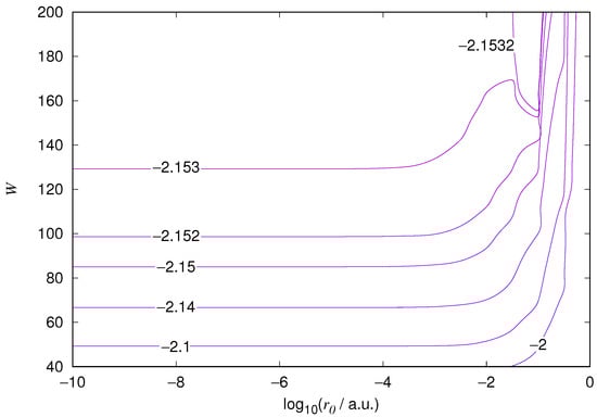
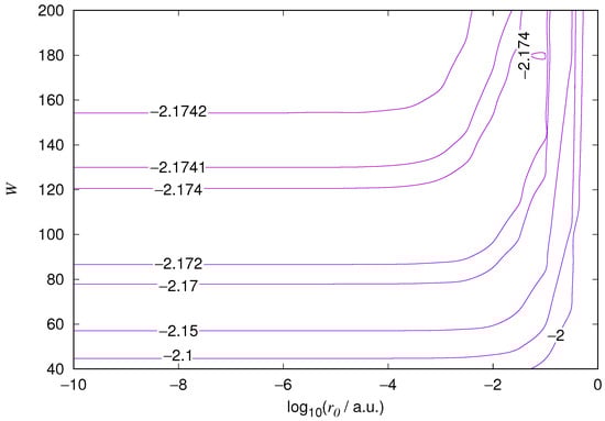
The results for the ground state of the hydrogen atom are presented in Figure 1 and Figure 2, for the 2s state in Figure 3 and Figure 4, and for the 2p state in Figure 5 and Figure 6. The results of the ground state of the helium atom are presented in Figure 7 and Figure 8. The results for $\mathrm{He}1\mathrm{s}2\mathrm{s}{}^1\mathrm{S}$ are given in Figure 9 and the results for $\mathrm{He}1\mathrm{s}2\mathrm{s}{}^3\mathrm{S}$ in Figure 10. As expected, the energy results are best for large values of W and small values of $r_0$. Using 200 basis functions for the helium ground state and computing the atom energies for $r_0={10}^k$, $k=-10,...,-1$ shows that atom energies are equal up to seven decimal places for $r_0\le {10}^{-6}$. Similar computation for the hydrogen 1s orbital shows that the H 1s energy is equal to $-0.5\mathrm{Ha}$ up to seven decimal places for $r_0\le 0.01$. For hydrogen 2s and 2p, the corresponding limit is $r_0\le 0.01$, too.

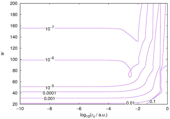
Figure 1. Hydrogen 1s orbital eigenenergy relative error. The $r_0$ is the EPP radius in atomic units and W is the basis size.

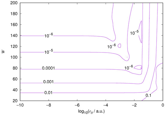
Figure 2. Relative error of the wavefunction value at the core radius for the hydrogen 1s orbital. Notations as in Figure 1.

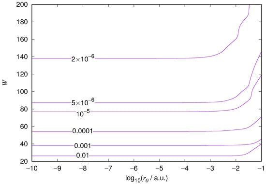
Figure 3. Hydrogen 2s orbital eigenenergy relative error. Notations as in Figure 1.

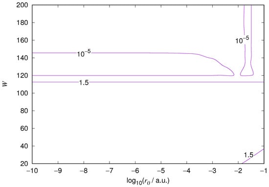
Figure 4. Relative error of the wavefunction value at the core radius for the hydrogen 2s orbital. Notations as in Figure 1.

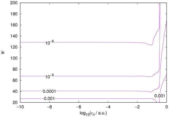
Figure 5. Hydrogen 2p orbital eigenenergy relative error. Notations as in Figure 1.

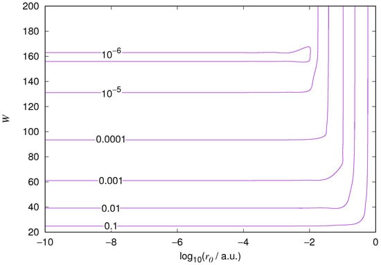
Figure 6. Relative error of the wavefunction value at the core radius for the hydrogen 2p orbital. Notations as in Figure 1.

Figure 7. The ground state energy of helium atom. The HF limit is given in Table 1. Notations as in Figure 1.

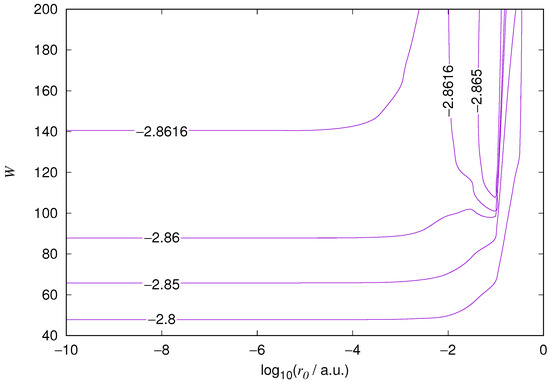
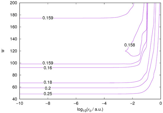
Figure 8. Relative error of the wavefunction value at the core radius for the 1s orbital of the ground state of the helium atom. Notations as in Figure 1.

Figure 9. Helium 1s2s ${}^1\mathrm{S}$ total energy. The HF limit is given in Table 1. Notations as in Figure 1.

Figure 10. Helium 1s2s ${}^3\mathrm{S}$ total energy. The HF limit is given in Table 1. Notations as in Figure 1.

We also found that when the number of basis functions is sufficiently large for a given system, there is an approximate threshold value so that reducing $r_0$ below it does not make the accuracy of the computed energy better. When the number of basis functions is sufficiently large and $r_0$ is sufficiently small, the hydrogenic orbitals are approximately continuous at $r_0$.

The most accurate computations are in the upper left corners of the figures. The orbitals of He 1s2s, except He 1s2s ${}^3\mathrm{S}$ 1s, are not continuous at all at $r_0$, and no continuity plots are presented for them. The computation results and exact results are given in Table 1. For the EPP–Galerkin method the best energies (largest basis and smallest $r_0$) of the computed systems are presented. The OIW–Galerkin results with same number of basis functions and grid spacing the same order of magnitude as for the most accurate EPP results are given, too. The accuracies of both of the methods depend on the grid spacing. The EPP–Galerkin method gives better results with the same number of basis functions and larger grid spacing. The results of the Finite Difference Method are also given. Note that for He 1s2s systems, the OIW–Galerkin method with a basis set of 601 functions and finest grid point distance $2^{-9}\mathrm{a}.\mathrm{u}.$ gives $E_{\mathrm{He}1\mathrm{s}2\mathrm{s}{}^1\mathrm{S}}=-2.153\mathrm{Ha}$ and $E_{\mathrm{He}1\mathrm{s}2\mathrm{s}{}^3\mathrm{S}}=-2.174\mathrm{Ha}$, which are approximately the same as the results of the EPP–Galerkin method.

Table 1. Hartree–Fock total energies of H and He occupation configurations. $E_{\mathrm{ref}}$ are chosen reference values. $E_{\mathrm{EPP}}$ is the energy given by the EPP–Galerkin-method, $h_{\mathrm{EPP}}$ is the grid spacing in the EPP–Galerkin method, $E_{\mathrm{OIW}}$ is the energy given by the OIW–Galerkin method, $E_{\mathrm{FDM}}$ is the energy given by the Finite Difference Method, and $N_{\mathrm{FDM}}$ is the number of grid points in the Finite Difference Method. For EPP, the most accurate results are given. For OIW computations, the number of basis functions is 201 and the finest grid spacing is $0.00625\mathrm{a}.\mathrm{u}$.

System	${\mathit{E}}_{\mathbf{ref}}/\mathbf{Ha}$	${\mathit{E}}_{\mathbf{EPP}}/\mathbf{Ha}$	${\mathit{h}}_{\mathbf{EPP}}/\mathbf{a}.\mathbf{u}.$	${\mathit{E}}_{\mathbf{OIW}}/\mathbf{Ha}$	${\mathit{E}}_{\mathbf{FDM}}/\mathbf{Ha}$	${\mathit{N}}_{\mathbf{FDM}}$
H 1s	$-0.5{*}^{†}$	−0.500000	0.075	−0.50	−0.49803	1001
H 2s	$-0.125{*}^{†}$	−0.125000	0.125	−0.125	−0.124741	2001
H 2p	$-0.125{*}^{†}$	−0.125000	0.125	−0.124998	−0.124995	2001
He $1{\mathrm{s}}^2$	$-2.8616800{}^{†}$ [8]	−2.8617	0.075	−2.834868	−2.839	1001
	$-2.903724*$ [9]
He $1\mathrm{s}2\mathrm{s}{}^1\mathrm{S}$	$-2.147{}^{\circ }$ [10]	−2.1532	0.1	−2.133579	−2.132	1001
	$-2.145974*$ [9]
He $1\mathrm{s}2\mathrm{s}{}^3\mathrm{S}$	$-2.171{}^{\circ }$ [10]	−2.1742	0.1	−2.154536	−2.155	1001
	$-2.175229*$ [9]

*: exact energy; ^†: HF limit; ∘: HF result.

Some of the computations using the diagonalization of the Hamiltonian operator yield an unphysical state for the minimum eigenvalue. For 1s and 2s orbitals, this eigenvalue seems to be about $-Z/r_0$ (in atomic units) and the corresponding eigenvector $v\left(\overline{P}\right)={(-{\delta }_{k,0})}_{k\ge 0}$. For the hydrogen 2p orbital, the unphysical eigenvector does not appear. The unphysical state remains the same during the HF iteration of $\mathrm{He}1{\mathrm{s}}^2$, $\mathrm{He}1\mathrm{s}2\mathrm{s}{}^1\mathrm{S}$, and $\mathrm{He}1\mathrm{s}2\mathrm{s}{}^3\mathrm{S}$. The physical admissibility of the wavefunctions $P_{nl}\left(r\right)$ was characterized by the condition

$$\underset{r\to 0}{lim}{P}_{nl}\left(r\right)=0.$$

(68)

We checked this condition by extrapolating solutions $P_{nl}\left(r\right)$ polynomially at $r=0$. Actually, we extrapolate polynomially $\overline{P}\left(s\right)$ at $s=-r_0$ using some points s near 0. Note that Fischer and Defranceschi [2] also find unphysical states in wavelet computations of hydrogen-like atoms. Their iteration scheme yields an unphysical result that is actually the mathematical ground state corresponding to the pseudopotential.

6. Discussion

The EPP–Galerkin method gives seven correct decimal places for the hydrogenic 1s orbital, six correct decimal places for the hydrogenic 2s and 2p orbitals, and four correct decimal places for He $1{\mathrm{s}}^2$. For He 1s2s ${}^1\mathrm{S}$ and ${}^3\mathrm{S}$, we obtain energies close to the HF limit. The OIW–Galerkin method with the finest grid spacing $0.0625\mathrm{a}.\mathrm{u}.$ gives energies with two to five correct decimal places. The grid size of OIW–Galerkin calculations is smaller compared to the EPP–Galerkin calculations. The Finite Difference Method yields rather inaccurate results even though the grid spacing is considerably smaller compared to the EPP–Galerkin calculations.

To our surprise, the EPP Hartree–Fock total energy of the He excited state configuration $1\mathrm{s}2\mathrm{s}{}^1\mathrm{S}$ is lower than the exact energy including correlations. This has been observed earlier in Ref. [10], and Cohen and Kelly [11] have shown that the reason is the nonorthogonality of this particular state and the ground state $1{\mathrm{s}}^2{}^1\mathrm{S}$. Thus, the kind of "orbital relaxation" of the excited HF state $1\mathrm{s}2\mathrm{s}{}^1\mathrm{S}$ lowers the total energy by mixing a little of the ground state with the excited state wave function. In the present case, the EPP overlap integral of these two states is 0.0274, and there are obvious ways to work out the pure excited states, but this is out of the scope of this study.

We were able to obtain results near the Hartree–Fock limit by using a large enough basis and small enough parameter $r_0$. It turns out that the EPP–Galerkin method yields better methods than the OIW–Galerkin method and considerably better results than the Finite Difference Method.

References

- Höynälänmaa, T.; Rantala, T.T.; Ruotsalainen, K. Solution of atomic orbitals in an interpolating wavelet basis. Phys. Rev. E 2004, 70, 066701. [Google Scholar] [CrossRef] [PubMed]
- Fischer, P.; Defranceschi, M. Numerical Solution of the Schrödinger Equation in a Wavelet Basis for Hydrogen-like Atoms. SIAM J. Numer. Anal. 1998, 35, 1–12. [Google Scholar] [CrossRef]
- Deslauriers, G.; Dubuc, S. Symmetric Iterative Interpolation Processes. Constr. Approx. 1989, 5, 49–68. [Google Scholar] [CrossRef]
- Chui, C.K.; Li, C. Dyadic affine decompositions and functional wavelet transforms. SIAM J. Math. Anal. 1996, 27, 865–890. [Google Scholar] [CrossRef]
- Donoho, D. Interpolating Wavelet Transforms; Department of Statitics, Stanford University: Stanford, CA, USA, 1992. [Google Scholar]
- Arias, T.A. Multiresolution analysis of electronic structure: Semicardinal and wavelet bases. Rev. Mod. Phys. 1999, 71, 267–311. [Google Scholar] [CrossRef]
- Cowan, R.D. The Theory of Atomic Structure and Spectra; University of California Press: Berkeley, CA, USA, 1981. [Google Scholar]
- Froese-Fischer, C. The Hartree–Fock Method for Atoms—A Numerical Approach; John Wiley & Sons: New York, NY, USA, 1977. [Google Scholar] [CrossRef]
- Drake, G.W. Atomic, Molecular, and Optical Physics Handbook; AIP Press: New York, NY, USA, 1996. [Google Scholar]
- Tang, T.L. Hartree-Fock Method for Helium Excited State. Available online: https://nukephysik101.wordpress.com (accessed on 22 October 2017).
- Cohen, M.; Kelly, P.S. Hartree–Fock Wavefunctions for Excited States: The 1S State of Helium. Can. J. Phys. 1965, 43, 1867–1881. [Google Scholar] [CrossRef]
Disclaimer/Publisher’s Note: The statements, opinions and data contained in all publications are solely those of the individual author(s) and contributor(s) and not of MDPI and/or the editor(s). MDPI and/or the editor(s) disclaim responsibility for any injury to people or property resulting from any ideas, methods, instructions or products referred to in the content. |
© 2023 by the authors. Licensee MDPI, Basel, Switzerland. This article is an open access article distributed under the terms and conditions of the Creative Commons Attribution (CC BY) license (https://creativecommons.org/licenses/by/4.0/).