Abstract
The large-scale grid connection of renewable energy causes great uncertainty in power system planning and operation. The power system flexibility index can quantify the system’s ability to adjust to uncertain events such as renewable energy, load fluctuations, and faults. Compared with traditional planning methods, the flexibility planning method can accurately evaluate the impact of various uncertain events on the system during the planning process, thus effectively ensuring the safe and economic operation of renewable energy systems. First, from the perspective of power transmission and safe operation, the flexibility index of the transmission line is defined. On this basis, considering the system’s economic operation strategy, aiming at the optimization of flexibility, investment cost, operation cost, and renewable energy consumption, a multi-objective transmission grid planning model based on flexibility and economy is proposed. The NSGAII optimization algorithm is used to solve the model. Finally, the simulation is performed in the modified Garver-6 and IEEE RTS-24 node systems to analyze the effectiveness of the proposed model. The results show that the planning model can meet the needs of flexibility and economy, improve the transmission capacity of power grids, reduce the probability of renewable energy abandonment or exceeding power flow, as well as enhance the flexibility, economy, and reliability of power systems.
1. Introduction
Because of traditional energy depletion and environmental degradation, large-scale renewable energy integration will become the development direction of future power systems [1,2]. However, the controllability of renewable energy such as wind power and photovoltaics is poor. Its spatial- temporal distribution characteristics and uncertainty have brought great challenges to the safe and economic operation of systems [3,4,5]. The flexibility index can quantify the power system’s ability to respond economically and reliably to uncertain events such as renewable energy, load fluctuations, and faults. In order to improve the renewable energy consumption rate and enhance the economics of high-ratio renewable energy power systems, it is of great significance to study system planning considering flexibility [6,7].
Nowadays, China’s renewable energy installed capacity has been at the forefront of the world, but at the same time, energy abandonment is also serious. In different regions, the reasons for energy abandonment are various. For example, the main reason for wind abandonment in Liaoning, Jilin, and Heilongjiang power grids is the lack of peak shaving capacity, while the main energy abandonment reason for power grids in Inner Mongolia, and Gansu is the insufficient transmission channel capacity [8]. However, the basic cause is insufficient system flexibility. The former is due to insufficient power supply flexibility, while the latter is due to insufficient power grid flexibility [9]. Flexibility is an important attribute that characterizes the ability of a power system to deal with uncertain events. Insufficient system flexibility will inevitably cause renewable energy abandonment. In the high-ratio renewable energy power system, sufficient flexible regulation capability will become a necessary condition for grid operation.
At present, the research on power system flexibility is in the primary stage, and the definition of flexibility is still constantly developing and improving. The International Energy Agency (IEA) defines flexibility as the ability of the power system to respond to predictable and unpredictable events [10], and the North American Electric Reliability Corporation (NERC) defines it as the ability of system resources to meet changes in demand [11]. Although the expressions are different, in general, power system flexibility can be described as the system’s ability to withstand uncertain events. Nowadays, experts and scholars have begun a series of studies on power system flexibility. References [12,13,14] preliminarily elaborate the concept of flexibility and propose a grid flexibility assessment method considering the flexibility direction. Reference [15] proposes a quantitative evaluation index system for flexibility from the perspective of reliability and statistics. In addition, there are also references that use the technical uncertainty scenarios flexibility index-technical economic uncertainty scenarios flexibility index (TUSFI-TEUSFI) [16], power spectral density [17], and other methods to evaluate the flexibility. The existing research including the above references has made many beneficial attempts to construct the flexibility index. However, it mainly focuses on the concept interpretation of flexibility and the improvement of evaluation methods, and less on the use in system planning and operation [18].
In the planning of a high-ratio renewable energy power grid, there have been many research results. Reference [19] applies a robust optimization method to power grid planning, and improve the power grid’s renewable energy consumption capacity by ensuring the system’s robust safety in extreme scenarios. Reference [20] builds a robust optimization model for energy storage and transmission joint planning with the minimum power shortage as the optimization goal. However, the above methods are often too conservative, and the balance between the economics and robustness of the planning scheme is difficult to control. In addition, reference [21] proposes a power grid planning method based on situational awareness technology. It designs system planning through four stages: situational awareness, situational understanding, situational presentation and prediction, and situational guidance. Reference [22] proposes applying an energy storage system to transmission grid planning, and obtains the optimal planning solution by establishing a mixed integer linear programming model. However, references [21,22] both take economic indicators such as system construction cost, operating cost, and penalty cost as optimization goals. The optimization model lacks quantification of the system’s ability to withstand uncertain events such as renewable energy fluctuations. While the planning scheme achieves the best economics, its margin for responding to uncertain events is often inadequate. In the planning method based on flexibility, reference [23] proposes a criterion for evaluating the flexibility of the power generation system and establishes a generator planning method that considers the uncertainty. Reference [24] proposes the concept of flexible supply and demand balance, and calculates the optimal system planning through the collaborative optimization of flexibility and economy. All the above research quantifies the ability of systems to resist uncertain events with flexibility indicators. Through multi-objective optimization, the balance between system flexibility and economy is effectively achieved. The planning scheme will neither lead to poor economy due to conservativeness, nor will it make the system operation risk uncontrollable in order to achieve optimal economic efficiency. However, the above studies are all planned from the perspective of power supply flexibility, and the research on power grid flexibility has not been deep enough. In fact, as far as the current research is concerned, the research on flexibility mainly focuses on the establishment of a flexibility index and the proposal of an evaluation method [24]. Only a few literature studies consider the application of flexibility in power system planning, and most of them are based on power supply flexibility. There are few transmission line planning methods which consider the power grid flexibility index.
Therefore, this paper proposes a method for transmission network expansion planning based on flexibility and economy. First, the flexibility evaluation indicators considering the power gird transmission capacity are established. Then based on the proposed flexibility index, with the objective of minimum investment construction cost, operating cost, and optimal flexibility, a multi-objective double-layer optimization model of the transmission network is constructed. The NSGAII optimization algorithm is used to solve the model, and the Pareto non-inferior solution is selected through the fuzzy membership function. Thus, a transmission line planning scheme with optimal flexibility and economy is obtained. Finally, the simulation of the modified Garver-6 and IEEE RTS-24 node systems verifies the feasibility and effectiveness of the proposed model.
The rest of the paper is organized as follows: Section 2 first introduces the grid flexibility evaluation method mentioned in this paper. The grid flexibility index is proposed from three aspects: line load rate during the normal operation state, line load rate and severity of line overload during the N-1 operation state. Section 3 proposes a planning model considering flexibility and economy, and specifies the model optimization objective and constraints. Section 4 introduces the model solving method. Finally, the case study and comparison results of the proposed model are shown in Section 5, and Section 6 contains the conclusion.
2. Power Grid Flexibility Index Evaluation
2.1. Analysis of the Main Factors Affecting Power Grid Flexibility
There are usually two reasons that lead to a power system’s load shedding and renewable energy abandonment: one is that the adjustment capacity of controllable units such as generators and energy storage systems cannot suppress the renewable energy output fluctuations, which is the power supply flexibility insufficiency; the other is the transmission congestion caused by the lack of transfer capability, which is the power grid flexibility insufficiency. Therefore, the power transmission ability is the main factor affecting the grid flexibility index. In addition, in actual operation, it is necessary to meet the N-1 safety constraint to ensure that the power flow does not exceed the capacity limit if a line is disconnected. Generally, the operation mode that satisfies the line capacity constraint but does not satisfy the N-1 constraint cannot be adopted by the system. Hence when evaluating the flexibility of transmission lines, the N-1 safety verification is also an index that must be considered.
2.2. Power Grid Flexibility Index during the Normal Operation State
Load rate can effectively measure the line transfer capability. Low line load rate can guarantee a greater line capacity margin. The system power flow dispatching ability will also be better [25]. Therefore, load rate can be used as an index to evaluate the power grid flexibility. However, the system has different flexibility requirements for different lines, thus this paper introduces a flexibility weighting coefficient. Define the line flexibility index of the normal operating state at time t as:
where, Ω1 is the set of flexibility evaluation lines, which is composed of N lines with the largest load rate; T is the set of flexibility evaluation moments; Ll(t) is the load rate of the lth line at time t; Pl(t) and Pl,max are the current transmission power and maximum transmission capacity of the lth line; μl is the flexibility weighting coefficient of line l.
The definition of flexibility weighting coefficient is shown in Equation (3):
where, is the average load rate of line i in T time period;
The flexibility weighting coefficient μi is equal to the proportion of line i load rate fluctuation variance in the total variance of all line load rate fluctuations. When the node injection power changes, the more drastic the line power flow changes, the greater the coefficient. It can reflect the ability of the line to resist power flow fluctuations, and then identify the lines that really restrict the power grid flexibility.
The meaning of the line flexibility index is the weighted sum of line load rate at time t. It can reflect the margin of system power flow dispatching capacity. The smaller the index, the better the power grid flexibility. Thus, the maximum in T time period is defined as the system normal power grid flexibility index:
where, is the system normal power grid flexibility index.
2.3. Power Grid Flexibility Index during the N-1 Operation State
N-1 safety constraints have a significant influence on the grid power transmission capacity. Hence it is necessary to consider the N-1 safety verification for transmission network planning. When the kth line at time t is disconnected, the line overflow flexibility index is defined as:
where, αi is the overflow flexibility weighting coefficient; is the ith line calculated load rate when the kth line at time t is disconnected, which can be greater than 1; the physical meaning of is to evaluate the severity of the N-1 state line limit violation. When there are more lines that exceed the line capacity limit, and the line exceeds the limit more seriously, the index is larger.
According to , the definition of the N-1 line over-limit flexibility index at time t is:
where, Ω2 is the line set for N-1 verification; φk is the probability of line k disconnected in T time period; ψk is the proportion of the probability that the line k is broken in all possible disconnections.
The above flexibility index can reflect the severity of line over-limit, but it cannot reflect the margin of grid flexibility in the N-1 operation state. Therefore, the N-1 line flexibility index at time t is defined as:
where, is the power grid average load rate when the line k is disconnected at time t; Ω3 is the set of lines participating in the N-1 line flexibility evaluation; NL is the number of lines in Ω3.
The physical meaning of is to evaluate the transmission capacity margin of the power grid in the N-1 state. The lower the load rate of each line in the N-1 state, the smaller the index. Therefore, the N-1 gird over-limit flexibility index and N-1 power grid flexibility index of the system in T time period are defined, as shown in Equation (11) and Equation (12).
where, is the system N-1 grid over-limit flexibility index; N-1 grid flexibility index.
2.4. N-1 Operation State Power Flow Calculation
In order to improve the calculation speed, this paper uses DC power flow break analysis to calculate the power flow in the N-1 state. Assuming that the injected power of each node is unchanged, when the branch km between node k and node m is disconnected, the power flow constraint equation becomes:
where, P0, θ0, and B0 are the node injection power vector, the node voltage phase angle vector, and the node DC power flow susceptance matrix under normal operating conditions; B1 and θ1 are the DC power flow susceptance matrix and node voltage phase angle vector under N-1 operating state; and are the variation of the susceptance matrix and the variation of the node voltage phase angle vector.
Because , and can be expressed by Equation (14):
where, bkm is the susceptance of the disconnected branch. The node admittance matrix after the branch km is disconnected can be written as:
According to the matrix inversion formula, Equation (15) can be written as:
Because of , the phase angle change of each node can be calculated by (18):
Therefore, the power flow through branch ij in N-1 state is:
where, Bij is the negative value of the susceptance of line ij, θi and θj are the voltage phase angles of node i and node j.
3. Power Grid Planning Model Based on Flexibility and Economy
3.1. Optimize Model Structure
In this paper, based on the proposed grid flexibility index, a two-level planning model of the power transmission network is established with economy and flexibility as optimization objectives.
The upper layer is the planning decision layer. This layer uses the economic index and flexibility index as optimization goals, and the lines to be built as the decision variables to determine the power grid topology. Then the grid parameters are transferred to the lower layer in the form of a system admittance matrix. The lower layer is the operation simulation layer. This layer aims at the optimal operation economy, conducts a multi-scenario system simulation operation under the grid structure determined by the upper layer, and obtains the optimal scheduling strategy under each scenario. Then the system operating parameters are returned to the upper level. Based on the parameters obtained by the lower layer, the upper layer calculates the economic index and flexibility index of the plan and optimizes the planning scheme.
The model realizes the optimal solution of the planning scheme through a continuous iteration process of the upper and lower layers. The planning model structure is shown in Figure 1.
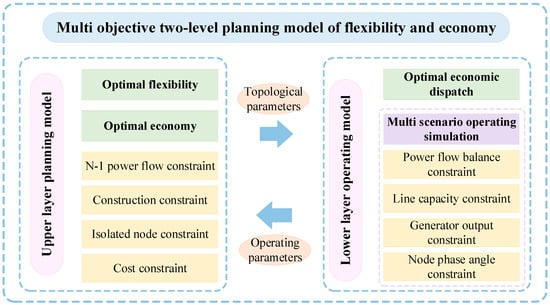
Figure 1.
Two-level planning model.
3.2. Upper Layer Planning Model
The upper layer is a multi-objective optimization model. The optimization objectives are divided into three parts: total annual planning cost Ctotal, normal power grid flexibility index , N-1 power grid flexibility index while the total annual planning cost Ctotal is composed of the equivalent annual construction cost Ccons and the annual operating cost Coper.
The objectives of the upper layer planning model are:
where, s is the lower layer operating scenario, S is the operating scenario set, ξs is the occurrence probability of scenario s; Coper,s, and are the sth scenario annual operating cost and flexibility indexes; r is the discount rate, n is the service life of the project, K is the fixed annual operating rate of the project; cline,ij is the construction cost of a new line between nodes i and j; xij is the number of new-built lines; Zij is a 0–1 decision variable, 0 means that the line to be built is not selected, 1 means that the line to be built is selected; Γ is the set of existing nodes and nodes to be expanded.
Equation (20) is the objective function of upper layer planning. Equation (21) is the specific function expression of each objective. Equation (22) is the calculation formula for the equivalent annual construction cost Ccons.
The constraints of the upper layer planning model are:
where, xij,max and xij,min are the upper and lower construction number limits of the line between nodes i and j, is the number of existing lines between nodes i and j; Ccons,max is the upper limit of the equivalent annual construction cost.
Equation (23) is the constraint of line construction. Equation (24) is the constraint of isolated nodes. Equation (25) is the cost constraint of the planning scheme. Equation (26) is the constraint of N-1 power flow limit, which is the constraint to ensure that the power flow does not exceed the limit if a line is disconnected.
3.3. Lower Layer Operating Model
The fundamental purpose of improving the power grid flexibility is to enhance the system’s renewable energy accommodation capability. Therefore, the lower layer operation model aims at minimizing the annual operation cost Coper,s of each scenario, and performs the optimal economic system scheduling. The Coper,s is composed of power generation cost CG,s and penalty cost Cpenalty,s. The objective function of the lower operating model is:
where: Pg,s(t) is the output power of the generator g at time t in the sth scenario; ag, bg, cg are the cost coefficients, кi is the ith renewable energy abandoned penalty coefficient; and are the maximum generating capacity and actual output of the ith renewable energy at time t in the sth scenario; G is the set of generators, Gre is the set of renewable energy.
The constraints of the lower layer operating model are:
where, B is the admittance matrix, θs is the node voltage phase angle vector in scenario s, PG,s is the output vector of generators, PRE,s is the output vector of the renewable energy, PL,s is the load power vector; Pij,max is the maximum transmission power of a single line in branch ij, Pij,s(t) is the total transmission power of branch ij at time t in the sth scenario; Pg,max and Pg,min are the upper and lower output limits of generator g; rg is the ramp rate, is the scheduling time interval; θi,max and θi,min are the upper and lower phase angle limits of node i, θi,s(t) is the phase angle of node i at time t in the sth scenario.
Equation (29) is the power flow balance constraint; Equation (30) is the line capacity constraint; Equation (31) is the generator output constraint; Equation (32) is the node voltage phase angle constraint.
4. Multi-Objective Programming Model Solution
4.1. Model Solving Algorithm
For the above multi-objective two level planning model, this paper uses the NSGAII optimization algorithm for solving. The NSGAII algorithm is an improved multi-objective genetic algorithm based on the NSGA algorithm. The optimization result is an optimal solution set, and each solution in the set is a Pareto non-inferior solution which does not dominate the others. Since the NSGAII algorithm does not need to determine the weight of each goal during optimization, it can avoid subjective interference in the optimization process [26]. Besides, the algorithm uses the non- dominated method for quick sorting and adopts the elite strategy and crowding degree to screen the population. Therefore, it has a good performance in maintaining population diversity and the convergence speed of solutions [27]. The NSGAII solution process of the planning model proposed in this paper is shown in Figure 2, while in the individual optimization objectives calculation, the optimization model described in the third section is used for the upper and lower layer transfer calculation.
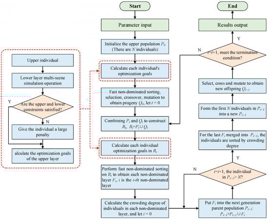
Figure 2.
Model solution flowchart.
4.2. Optimal Solution Calculation
The optimization result of the NSGAII algorithm is a Pareto optimal solution set, and all solutions in the set are not dominated by each other. Therefore, the decision maker can calculate the optimal compromise solution as the final optimization scheme according to different actual conditions [28]. This paper uses the fuzzy membership function described in [28] to select the final optimization planning. The degree of membership of the nth objective function in the mth solution in the Pareto solution set is defined as:
where, is the degree of membership, is the value of the nth objective function in the mth solution, and are the upper and lower limits of the objective function.
According to the calculation results of each objective, the membership degree weighted value um of the mth solution is defined as:
where, ωn is the weighting coefficient of the nth objective function, Nf is the number of objective functions, and Nm is the number of Pareto non-inferior solutions.
Finally, the membership weighted values of each solution in the Pareto optimal solution set are compared. The solution with the largest um is the final optimized solution.
5. Case Study
This paper uses the modified Garver-6 and IEEE RTS-24 node systems to verify the effectiveness and feasibility of the proposed grid planning model. The simulation parameters are as follows: the line construction cost per unit length cline = 2 × 10⁵ $/km, the renewable energy abandoned penalty coefficient κi = 63.3 $/MWh, the discount rate r = 10%, the project service life n = 15 years, the project fixed annual operating rate K = 10%. The flexibility evaluation line set Ω1/Ω3 selects the 30% lines with the largest load rate in the grid and the disconnection probability of each line is the same. In addition, the load data of each node is defined as the product of the maximum node load and the load per unit value in each scenario. The maximum output of each node’s renewable energy is the product of the node’s renewable energy installed capacity and the per unit value of renewable energy output in each scenario. The per unit value of load and renewable energy output are obtained from the actual data of a power grid in southern China by K-means algorithm clustering.
5.1. Garver-6 System
The Garver-6 system has 5 primitive nodes, 1 expansion node and 15 expandable transmission channels. Each transmission channel can build 4 lines at most. The specific data of the modified Garver-6 system is in Table A1, Table A2 and Table A3 of Appendix A.
5.1.1. The Deterministic Economic Planning
In order to verify the correctness of the model, this section does not consider the connection of renewable energy temporarily, and only takes the economy as the optimization objective. The generator output and load are the same as those in reference [21] and [29]. The power grid planning scheme obtained by the proposed model is: l3–5 = 1, l2–6 = 4, l4–6 = 2 and l3–5 = 1 means one transmission line built between node 3 and node 5. The planning scheme is the same as that obtained by the mixed integer programming method in reference [21] or other methods in reference [29], which verify the correctness of the model proposed in this paper.
5.1.2. The Flexibility Planning
The 360 MW conventional generator in node 3 is replaced with an equal capacity wind turbine, the system balance node is changed to node 1, and other parameters remain unchanged. Based on wind power peak-valley output, load peak-valley output, four typical scenarios are selected by permutation and combination for the lower layer operation simulation. The scheduling step size is 2 h. Load and wind power data is shown in Figure A1 of Appendix A.
In the planning model, the total planning cost Ctotal is taken as the economic target, and the normal power grid flexibility index is taken as the flexibility target to optimize the solution, while the N-1 power grid flexibility index is not considered temporarily. The upper limit of the equivalent annual construction cost Ccons is set to 40 million US dollars, the population number of NSGAII optimization algorithm is set to 100, and the iteration is 200 generations. The Pareto non-inferior solution frontier of the planning result is shown in Figure 3.
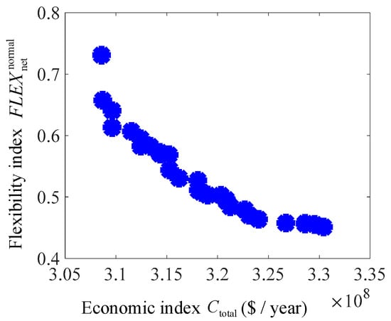
Figure 3.
Flexibility–Economy pareto frontier.
This paper temporarily considers that the flexibility index and the economic index are equally important, and the weighting coefficient of the economic and flexibility indexes are both set to 0.50. The optimal power grid planning obtained according to the fuzzy membership function is as follows: l2–3 = 1, l2–6 = 4, l3–5 = 3, l4–6 = 3. In order to analyze the impact of flexibility on power grid planning, this section also calculates the traditional economic planning with the minimum construction cost as the goal. The optimal planning scheme is l2–6 = 3, l3–5 = 1, l3–6 = 1, l4–6 = 2. The comparison results of the two planning schemes are shown in Table 1.

Table 1.
Comparison of planning scheme results in typical scenarios.
It can be seen from Table 1 that the flexibility planning has effectively improved the flexibility of the power grid. In terms of economic indicators, although flexibility planning has a 33.03% increase in construction costs compared to economic planning, due to the increased flexibility, the system’s ability to accommodate renewable energy has been improved. Considering the renewable energy abandoned penalty cost, the annual total cost Ctotal of flexibility planning has been reduced.
Take scenario 1 as an example to illustrate the comparison between the two planning schemes. Define the lines that load rate exceeds 0.8 as heavy-load lines. Figure 4 shows the highest grid line load rate of the two planning schemes. Figure 5 shows the change in the number of heavy-load lines. It can be seen that with the gradual increase of the system load, the economic planning began to see heavy-load lines, even full-load lines. The maximum line load rate of the flexibility planning is 0.76, and there is no heavy-load line, so it can ensure the flexibility of the system and the ability of the power flow scheduling.
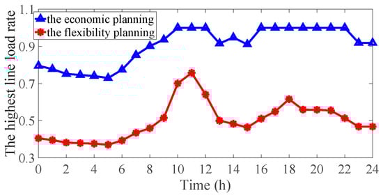
Figure 4.
The highest line load rate of the power grid.
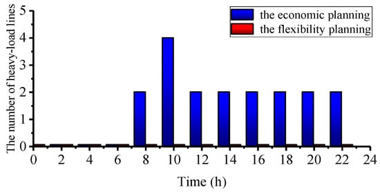
Figure 5.
The number of heavy-load lines.
In terms of renewable energy consumption capacity, set the wind power output fluctuation range to [0, 0.5] and load fluctuation range to [−0.3, 0.3]. Ten uniform samples are taken in the above two intervals, and the sampling results are superimposed on the wind power and load per unit values of scenario 1, thus forming 10 random scenarios. The specific data is shown in Figure A2 of Appendix A. The annual renewable energy abandoned penalty costs of the two planning schemes in the above 10 random scenarios are shown in Figure 6. It can be seen that the penalty cost for economic planning is about 16.6 million dollars, while the flexibility plan is only about 1.7 million dollars, which reduces the renewable energy abandonment by 89.7%. It shows that after the power grid flexibility is improved, the system has excellent adaptability to the uncertain power fluctuations, thus ensuring the consumption of renewable energy.
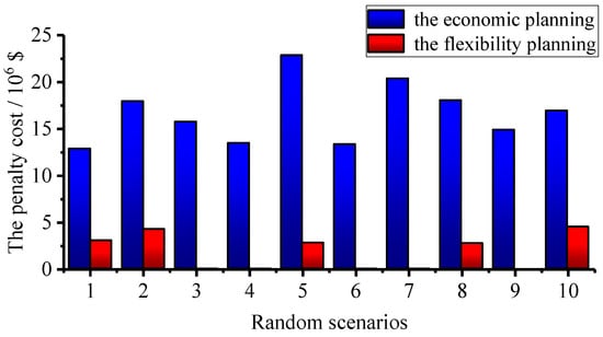
Figure 6.
The renewable energy abandoned penalty costs in random scenarios.
5.2. IEEE RTS-24 System
Suppose that in a future planning level year, the capacity of all loads, generators, and transformers of the IEEE RTS-24 system will increase to three times of the current value, and the line capacity will increase to two times of the current value. In addition, the traditional generators in nodes 1, 13, 21, and 22 are all converted into wind, photovoltaic, and hydropower units with the same total capacity. The system total installed capacity of wind, photovoltaic, and hydropower units is 3321 MW, and the penetration rate of renewable energy is about 32.5%. Since the overall load rate of the system is relatively low and the grid flexibility is relatively abundant in the load valley period, this section selects two typical scenarios of renewable energy output peak period, valley period and load peak period for the lower layer operation simulation. The data of modified IEEE RTS-24 system is shown in Table A4, Table A5 and Table A6 of Appendix B. The data of renewable energy, load per unit value is shown in Figure A3 of Appendix B.
In the planning model, the total planning cost Ctotal is taken as the economic optimization objective, and the normal, N-1 power grid flexibility index , are taken as flexibility optimization objectives for three-dimensional optimization. Because strict N-1 verification needs to break all lines, the calculation workload will be complex when the population scale is large or the iteration number is large. Considering that meaningful disconnection verification only occupies a part of the entire line set, most of the lines will not cause system overload after disconnection. Therefore, in order to reduce the computational complexity, only the lines with high overload possibility could be selected [30]. In this paper, the top 30% of the lines with the highest transmission power are selected for N-1 verification during the iterative process. The limit of Ctotal is set to 40 million dollars, the population number of the NSGAII optimization algorithm is set to 100, and the iteration is 400 generations. The Pareto non-inferior solution frontier of the planning result is shown in Figure 7.
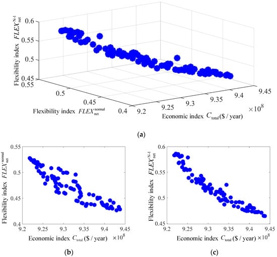
Figure 7.
Flexibility–Economy Pareto Frontier. (a) The total planning cost—Normal power grid flexibility index—N-1 power grid flexibility index Pareto Frontier; (b) projection; (c) projection.
Figure 7 shows the changing trend between economic indicators and flexibility indicators. It can be seen that as the total planning cost Ctotal increases, the power grid flexibility indexes and gradually decrease, and the system flexibility becomes better. The economic and flexibility weighting coefficients are still set to 0.5 (the normal and N-1 grid flexibility index weighting coefficients are both 0.25). The optimal planning scheme obtained by the fuzzy membership function is called Plan A. For comparison, this section also calculates the dual objective grid planning with the optimization objectives of economy and normal grid flexibility. The optimal plan is called Plan B. The calculation formula of penalty cost Cov for line exceeding limit is shown in Equation (35). Where, Pk,ov(t) is the overload power of the grid when the line k is broken at time t; кov is the penalty coefficient, which is 10,000 $/MW [24]; The probability of line disconnection is 3%. The comparison results of Plan A/B are shown in Table 2.
Table 2.
Comparison of planning scheme results under typical scenarios.
It can be seen in Table 2 that since the normal power grid flexibility index is considered in Plan A and Plan B, both of them can achieve complete consumption of renewable energy under normal operation, and the renewable energy abandonment penalty cost Cpenalty is 0. However, Plan A also considers the N-1 grid flexibility index , so it can avoid transmission power out of the capacity limit during N-1 faults and greatly improve the safety and reliability of the power grid. Considering that the power system may need to ensure N-1 safety constraints during normal operation, Plan A can better ensure the consumption of renewable energy.
Figure 8a shows the change of the maximum line load rate of the entire network under the normal operation state of Plan A/B. It can be seen that the whole network maximum line load rate of the two schemes is less than 0.8, and the power grid flexibility is relatively sufficient. Figure 8b shows the highest line load rate of the entire network under the most severe N-1 operating state. Due to the consideration of the N-1 flexibility index, the highest load rate of Plan A is 0.954, and no limit violation occurs. In contrast, the highest load rate of Plan B is generally above 1.2. Therefore, by comprehensively considering the economy, the normal power grid flexibility and the N-1 grid flexibility, the economical and reliable consumption of renewable energy in the power system can be achieved.
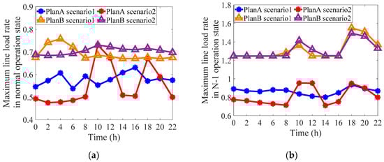
Figure 8.
The changing of the highest line load rate. (a) Normal load rate; (b) N-1 load rate.
6. Conclusions
In the context of large-scale renewable energy integration, it becomes more and more important to enhance the power system flexibility. In order to meet the demand of the power grid for flexibility, this paper proposes a method for transmission grid expansion planning of renewable energy power system based on flexibility and economy. First, this paper puts forward the grid flexibility evaluation indicators under normal operating state and N-1 operating state respectively. Then based on the mentioned indicators, a multi-level transmission line planning model considering flexibility and economy is constructed. Finally, the NSGAII algorithm is used to solve the model, thus achieving the multi-objective optimization of flexibility and economy. Using the modified Garver-6 and IEEE RTS-24 node systems for simulation, the following conclusions are obtained:
(1) The proposed model is applicable to both flexible and economic multi-objective grid planning, as well as traditional single-economic target grid planning. (2) Compared with traditional planning methods, the planning model proposed in this paper can effectively improve the power grid flexibility, thereby preventing the abandonment of renewable energy due to line congestion. (3) The reliability of the model is greatly enhanced due to the addition of the N-1 flexibility index. Considering that the system may need to ensure N-1 safety constraints during normal operation, the model corresponds more to engineering reality. The planning results can more safely and effectively improve the renewable energy consumption rate of the power system.
Author Contributions
Conceptualization, Z.C. and Y.H.; Formal analysis, Z.C.; Methodology, Z.C.; Software, Z.C.; Supervision, X.T.; Validation, G.Y.; Visualization, Z.C.; Writing—original draft, Z.C.; Writing—review and editing, N.T. All authors have read and agreed to the published version of the manuscript.
Funding
This research is funded by National Key Research and Development Program under grant number 2017YFB0903202; China Southern Power Grid Major Project under grant number YNKJXM20170008; 2019 Major Research and Innovation Project of Shanghai Municipal Education Commission under grant number 2019-01-07-00-02-E00044.
Acknowledgments
The author acknowledges the experimental data provided by the Yunnan power grid company.
Conflicts of Interest
The authors declare no conflict of interest.
Nomenclature
| Parameters | |
| the maximum transmission capacity of the lth line | |
| the average load rate of the ith line in T time period | |
| the flexibility weighting coefficient of the lth line | |
| the overflow flexibility weighting coefficient | |
| the probability of the kth line disconnected in T time period | |
| the number of lines in Ω3 | |
| the discount rate | |
| the service life of the project | |
| the fixed annual operating rate of the project | |
| the construction cost of a new line between nodes i and j | |
| the number of existing lines/new-built lines between nodes i and j | |
| the upper/lower limit of the construction line between nodes i, j | |
| the occurrence probability of sth scenario | |
| the gth generator cost coefficient | |
| the ith renewable energy abandoned penalty coefficient | |
| the overflow penalty coefficient | |
| the ramp rate | |
| the scheduling time interval | |
| the maximum transmission power of a single line in branch ij | |
| the upper/lower output limit of generator g | |
| the upper/lower phase angle limit of node i | |
| the upper/lower limit of the objective function | |
| the weighting coefficient of the nth objective function | |
| the number of objective functions | |
| the number of Pareto non-inferior solutions | |
| Variables | |
| the current transmission power of the lth line at time t | |
| the load rate of the lth line at time t | |
| the ith line calculated load rate when the kth line is disconnected | |
| the line flexibility index of the normal operating state at time t | |
| the line overflow flexibility index when the kth line is disconnected | |
| the power grid average load rate when the kth line is disconnected at time t | |
| the N-1 line over-limit flexibility index at time t | |
| the N-1 line flexibility index at time t | |
| the system normal power grid flexibility index | |
| the N-1 gird over-limit flexibility index | |
| the N-1 power grid flexibility index | |
| the node injection power vector/the node voltage phase angle vector/the DC power flow susceptance matrix under normal operating state | |
| the node voltage phase angle vector/the DC power flow susceptance matrix under N-1 operating state | |
| the node voltage phase angle vector/the susceptance matrix variation | |
| the output vector of generators/renewable energy/load power | |
| the total annual planning cost | |
| the equivalent annual construction cost | |
| the annual operating cost | |
| the upper limit of the equivalent annual construction cost | |
| the power generation cost in the sth scenario | |
| the penalty cost in the sth scenario | |
| the output power of the generator g at time t in the sth scenario | |
| the maximum/actual generating capacity of the ith renewable energy at time t in the sth scenario | |
| the total transmission power of branch ij at time t in the sth scenario | |
| the overload power of the grid when the line k is broken at time t | |
| the phase angle of node i at time t in the sth scenario | |
| the mth solution membership degree of the nth objective function | |
| the value of the nth objective function in the mth solution | |
| Sets | |
| T | the set of flexibility evaluation moments |
| the set of flexibility evaluation lines | |
| the line set for N-1 verification | |
| the set of lines participating in the N-1 line flexibility evaluation | |
| the set of system existing nodes and nodes to be expanded | |
| the set of lower layer operating scenario | |
| the set of generators | |
| the set of renewable energy | |
Appendix A. The Modified Garver-6 Node System Related Data
Table A1.
Garver-6 system line data.
Table A1.
Garver-6 system line data.
| Number | Node Number | Reactance/pu | Capacity/MW | Length/km | The Number of Existing Lines | Maximum Number of Construction |
|---|---|---|---|---|---|---|
| 1 | 1–2 | 0.40 | 100 | 40 | 1 | 4 |
| 2 | 1–3 | 0.38 | 100 | 38 | 0 | 4 |
| 3 | 1–4 | 0.60 | 80 | 60 | 1 | 4 |
| 4 | 1–5 | 0.20 | 100 | 20 | 1 | 4 |
| 5 | 1–6 | 0.68 | 70 | 68 | 0 | 4 |
| 6 | 2–3 | 0.20 | 100 | 20 | 1 | 4 |
| 7 | 2–4 | 0.40 | 100 | 40 | 1 | 4 |
| 8 | 2–5 | 0.31 | 100 | 31 | 0 | 4 |
| 9 | 2–6 | 0.30 | 100 | 30 | 0 | 4 |
| 10 | 3–4 | 0.59 | 82 | 59 | 0 | 4 |
| 11 | 3–5 | 0.20 | 100 | 20 | 1 | 4 |
| 12 | 3–6 | 0.48 | 100 | 48 | 0 | 4 |
| 13 | 4–5 | 0.63 | 75 | 63 | 0 | 4 |
| 14 | 4–6 | 0.30 | 100 | 30 | 0 | 4 |
| 15 | 5–6 | 0.61 | 78 | 61 | 0 | 4 |
Table A2.
Garver-6 system generator data.
Table A2.
Garver-6 system generator data.
| Generator Number | G1 | WT1 | G3 |
|---|---|---|---|
| Generator access node | 1 | 3 | 6 |
| Generator capacity/MW | 150 | 360 | 600 |
| Ramp rate/(MW·h−1) | 40 | / | 120 |
| a/($·(MW2·h)−1) | 3.597 | / | 0.33 |
| b/($·(MW·h)−1) | 0 | / | 0 |
| c/($·h−1) | 0 | / | 0 |
Table A3.
Garver-6 system maximum node load.
Table A3.
Garver-6 system maximum node load.
| Node Number | Maximum Load/MW | Node Number | Maximum Load/MW |
|---|---|---|---|
| 1 | 80 | 4 | 160 |
| 2 | 240 | 5 | 240 |
| 3 | 40 | 6 | 0 |

Figure A1.
Typical load and wind power planning scenarios.
Probability of peak load occurrence: 0.6; Probability of valley load occurrence: 0.4; Probability of peak wind power occurrence: 0.7; Probability of valley wind power occurrence: 0.3.
Scenario 1-Probability of peak wind power and peak load: 0.42; Scenario 2-Probability of valley wind power and valley load: 0.12; Scenario 3-Probability of peak wind power and valley load: 0.28; Scenario 4-Probability of valley wind power and peak load: 0.18.

Figure A2.
Ten random scenarios of load and wind power.
Appendix B. The Modified IEEE RTS-24 Node System Related Data
Table A4.
IEEE RTS-24 system renewable energy data.
Table A4.
IEEE RTS-24 system renewable energy data.
| Number | Name | Generator Type | Generator Access Node | Generator Capacity/MW |
|---|---|---|---|---|
| 1 | PV1 | photovoltaic | 1 | 576 |
| 2 | WT1 | wind power | 15 | 645 |
| 3 | WT2 | wind power | 21 | 1200 |
| 4 | HT1 | hydropower | 22 | 900 |
Table A5.
IEEE RTS-24 system maximum node load.
Table A5.
IEEE RTS-24 system maximum node load.
| Node | Maximum Load/MW | Node | Maximum Load/MW | Node | Maximum Load/MW |
|---|---|---|---|---|---|
| 1 | 324 | 9 | 525 | 17 | 0 |
| 2 | 291 | 10 | 585 | 18 | 999 |
| 3 | 540 | 11 | 0 | 19 | 543 |
| 4 | 222 | 12 | 0 | 20 | 384 |
| 5 | 213 | 13 | 795 | 21 | 0 |
| 6 | 408 | 14 | 582 | 22 | 0 |
| 7 | 375 | 15 | 951 | 23 | 0 |
| 8 | 513 | 16 | 300 | 24 | 0 |
Table A6.
IEEE RTS-24 system line data.
Table A6.
IEEE RTS-24 system line data.
| Number | Node Number | Reactance/pu | Capacity/MW | Length/km | The Number of Existing Lines | Maximum Number of Construction |
|---|---|---|---|---|---|---|
| 1 | 1–2 | 0.0139 | 350 | 3 | 1 | 3 |
| 2 | 1–3 | 0.2112 | 350 | 55 | 1 | 3 |
| 3 | 1–5 | 0.0845 | 350 | 22 | 1 | 3 |
| 4 | 2–4 | 0.1267 | 350 | 33 | 1 | 3 |
| 5 | 2–6 | 0.192 | 350 | 50 | 1 | 3 |
| 6 | 3–9 | 0.119 | 350 | 31 | 1 | 3 |
| 7 | 3–24 | 0.0839 | 1200 | 0 | 1 | 0 |
| 8 | 4–9 | 0.1037 | 350 | 27 | 1 | 2 |
| 9 | 5–10 | 0.0883 | 350 | 23 | 1 | 2 |
| 10 | 6–10 | 0.0605 | 350 | 16 | 1 | 2 |
| 11 | 7–8 | 0.0614 | 350 | 16 | 2 | 2 |
| 12 | 8–9 | 0.1651 | 350 | 43 | 1 | 2 |
| 13 | 8–10 | 0.1651 | 350 | 43 | 1 | 2 |
| 14 | 9–11 | 0.0839 | 1200 | 0 | 1 | 0 |
| 15 | 9–12 | 0.0839 | 1200 | 0 | 1 | 0 |
| 16 | 10–11 | 0.0839 | 1200 | 0 | 1 | 0 |
| 17 | 10–12 | 0.0839 | 1200 | 0 | 1 | 0 |
| 18 | 11–13 | 0.0476 | 1000 | 33 | 1 | 3 |
| 19 | 11–14 | 0.0418 | 1000 | 29 | 1 | 3 |
| 20 | 12–13 | 0.0476 | 1000 | 33 | 1 | 3 |
| 21 | 12–23 | 0.0966 | 1000 | 67 | 1 | 3 |
| 22 | 13–23 | 0.0865 | 1000 | 60 | 1 | 3 |
| 23 | 14–16 | 0.0389 | 1000 | 27 | 1 | 4 |
| 24 | 15–16 | 0.0173 | 1000 | 12 | 1 | 3 |
| 25 | 15–21 | 0.049 | 1000 | 34 | 2 | 2 |
| 26 | 15–24 | 0.0519 | 1000 | 36 | 1 | 2 |
| 27 | 16–17 | 0.0259 | 1000 | 18 | 1 | 2 |
| 28 | 16–19 | 0.0231 | 1000 | 16 | 1 | 2 |
| 29 | 17–18 | 0.0144 | 1000 | 10 | 1 | 2 |
| 30 | 17–22 | 0.1053 | 1000 | 73 | 1 | 2 |
| 31 | 18–21 | 0.0259 | 1000 | 18 | 2 | 2 |
| 32 | 19–20 | 0.0396 | 1000 | 27.5 | 2 | 2 |
| 33 | 20–23 | 0.0216 | 1000 | 15 | 2 | 2 |
| 34 | 21–22 | 0.0678 | 1000 | 47 | 1 | 2 |

Figure A3.
Typical load and wind power planning scenarios. (a) Scenario 1, occurrence probability: 0.4603; (b) Scenario 2, occurrence probability: 0.5397.
References
- Jiang, W.; Yang, K.X.; Yang, J.J.; Mao, R.W.; Xue, N.F.; Zhuo, Z.H. A multiagent-based hierarchical energy management strategy for maximization of renewable energy consumption in interconnected multi-microgrids. IEEE Access 2019, 7, 169931–169945. [Google Scholar] [CrossRef]
- Jiang, L.P.; Wang, C.X.; Huang, Y.H.; Pei, Z.Y.; Xin, S.X.; Wang, W.S.; Ma, S.; Tom, B. Growth in wind and sun: Integrating variable generation in china. IEEE Power Energy Mag. 2015, 13, 40–49. [Google Scholar] [CrossRef]
- Yuan, X. Overview of problems in large-scale wind integrations. J. Mod. Power Syst. Clean Energy 2013, 1, 22–25. [Google Scholar] [CrossRef]
- Cheng, H.Z.; Li, J.; Wu, Y.W.; Chen, H.Y.; Zhang, N.; Liu, L. Challenges and prospects for ac/dc transmission expansion planning considering high proportion of renewable energy. Autom. Electr. Power Syst. 2017, 41, 19–27. [Google Scholar]
- Orfanos, G.A.; Georgilakis, P.S.; Hatziargyriou, N.D. Transmission expansion planning of systems with increasing wind power integration. IEEE Trans. Power Syst. 2013, 28, 1355–1362. [Google Scholar] [CrossRef]
- Zhao, J.; Zheng, T.; Litvinov, E.A. Unified framework for defining and measuring flexibility in power system. IEEE Trans. Power Syst. 2016, 31, 339–347. [Google Scholar] [CrossRef]
- Xu, T.H.; Lu, Z.X.; Qiao, Y.; An, J. High penetration of renewable energy power planning considering coordination of source-load-storage multi-type flexible resources. J. Glob. Energy Interconnect. 2019, 2, 27–34. [Google Scholar]
- Zhu, L.Z.; Chen, N.; Han, H.L. Key problems and solutions of wind power accommodation. Autom. Electr. Power Syst. 2011, 35, 29–34. [Google Scholar]
- Lu, Z.X.; Li, H.B.; Qiao, Y. Power system flexibility planning and challenges considering high proportion of renewable energy. Autom. Electr. Power Syst. 2016, 40, 147–158. [Google Scholar]
- IEA. Harnessing Variable Renewables; International Energy Agency: Paris, France, 2011; pp. 41–67. [Google Scholar]
- NERC. Special Report: Potential Reliability Impacts of Emerging Flexible Resources; North American Electric Reliability Corporation: Atlanta, GA, USA, 2010; pp. 2–6. [Google Scholar]
- Lannoye, E.; Flynn, D.; O’Malley, M. The role of power system flexibility in generation planning. In Proceedings of the 2011 IEEE Power and Energy Society General Meeting, Detroit, MI, USA, 24–28 July 2011. [Google Scholar]
- Lannoye, E.; Flynn, D.; O’Malley, M. Evaluation of power system flexibility. IEEE Trans. Power Syst. 2012, 27, 922–931. [Google Scholar] [CrossRef]
- Lannoye, E.; Flynn, D.; O’Malley, M. Transmission, variable generation, and power system flexibility. IEEE Trans. Power Syst. 2015, 30, 57–66. [Google Scholar] [CrossRef]
- Li, H.B.; Lu, Z.X.; Qiao, Y.; Zeng, P.L. Assessment on operational flexibility of power grid with grid-connected large-scale wind farms. Power Syst. Technol. 2015, 39, 1672–1678. [Google Scholar]
- Capasso, A.; Falvo, M.C.; Lamedica, R.; Lauria, S.; Scalcino, S. A new methodology for power systems flexibility evaluation. In Proceedings of the 2005 IEEE Russia Power Tech, St. Petersburg, Russia, 27–30 June 2005. [Google Scholar]
- Bouffard, F.; Ortega-Vazquez, M. The value of operational flexibility in power systems with significant wind power generation. In Proceedings of the Power and Energy Society General Meeting, Detroit, MI, USA, 24–28 July 2011. [Google Scholar]
- Wang, X.; Ye, X.; Tang, Q.; Zhang, Y.H.; Li, T.; Liu, W.Y.; Li, H.Q. Transmission network expansion planning based on generalized flexibility index system. Electr. Power Constr. 2019, 40, 67–76. [Google Scholar]
- Liang, Z.P.; Chen, H.Y.; Zheng, X.D.; Wang, X.J.; Chen, S.M. Robust expansion planning of transmission network considering extreme scenario of wind power. Autom. Electr. Power Syst. 2019, 43, 58–68. [Google Scholar]
- Alismail, F.; Xiong, P.; Singh, C. Optimal wind farm allocation in multi-area power systems using distributionally robust optimization approach. IEEE Trans. Power Syst. 2017, 33, 536–544. [Google Scholar] [CrossRef]
- Huang, Y.; Liu, B.Z.; Wang, K.Y.; Ai, X. Joint planning of energy storage and transmission network considering wind power accommodation capability. Power Syst. Technol. 2018, 42, 1480–1489. [Google Scholar]
- Shi, Z.P.; Wang, Z.M.; Wu, W.P.; Wang, X.R.; Hu, Z.C. Evaluation of renewable energy integration capability and network expansion planning based on situation awareness theory. Power Syst. Technol. 2017, 41, 2180–2186. [Google Scholar]
- Eduardo, A.M.C.; Tomislav, C.; Pierluigi, M. Flexible distributed multienergy generation system expansion planning under uncertainty. IEEE Trans. Smart Grid 2016, 7, 348–357. [Google Scholar]
- Liu, W.Y.; Li, H.Q.; Zhang, H.L.; Xiao, Y. Expansion planning of transmission grid based on coordination of flexible power supply and demand. Autom. Electr. Power Syst. 2018, 42, 56–63. [Google Scholar]
- Yu, H.B. Research of Power System Dispatching Strategy and Wind Power Planning Based on Load Rate Balance Degree. Master’s Thesis, Harbin Institute of Technology, Harbin, China, 2013. [Google Scholar]
- Deb, K.; Pratap, A.; Agarwal, S.; Meyarivan, T. A fast and elitist multiobjective genetic algorithm: NSGA-II. IEEE Trans. Evol. Comput. 2002, 6, 182–197. [Google Scholar] [CrossRef]
- Wang, J.; Zheng, X.D.; Tai, N.L.; Wei, W.; Li, L.F. Resilience-oriented optimal operation strategy of active distribution network. Energies 2019, 12, 3380. [Google Scholar] [CrossRef]
- Jiang, H.L.; An, X.; Wang, Y.W.; Qin, J.Z.; Qian, G.C. Improved nsga2 algorithm based multi-objective planning of power grid with wind farm considering power quality. Proc. CSEE 2015, 35, 5405–5411. [Google Scholar]
- Sun, H.B. Power Network Planning; Chongqing University Press: Chongqing, China, 1996. [Google Scholar]
- Ai, Q. Power System Steady State Analysis; Tsinghua University Press: Beijing, China, 2014. [Google Scholar]
© 2020 by the authors. Licensee MDPI, Basel, Switzerland. This article is an open access article distributed under the terms and conditions of the Creative Commons Attribution (CC BY) license (http://creativecommons.org/licenses/by/4.0/).