Low-Cost Multi-Objective Optimization of Multiparameter Antenna Structures Based on the l₁ Optimization BPNN Surrogate Model

Abstract

The development of modern wireless communication systems not only requires the antenna to be lightweight, low cost, easy to manufacture and easy to integrate but also imposes requirements on the miniaturization, wideband, and multiband design of the antenna. Therefore, designing an antenna that quickly and effectively meets multiple performance requirements is of great significance. To solve the problem of the large computational cost of traditional multi-objective antenna design methods, this paper proposes a backpropagation neural network surrogate model based on l₁ optimization (l₁-BPNN). The l₁ optimization method tends to punish larger weight values and select smaller weight values so as to preserve a small amount of important weights and reset relatively unimportant weights to zero. By using l₁ optimization method, the network mapping structure can be automatically adjusted to achieve the most suitable and compact structure of the surrogate model. Furthermore, for multi-parameter antenna design problems, a fast multi-objective optimization framework is constructed using the proposed l₁-BPNN as a surrogate model. The framework is illustrated using a miniaturized multiband antenna design case, and a comparison with previously published methods, as well as numerical validation, is also provided.

1. Introduction

With the rapid development of radio communication technologies, wireless communication devices are becoming more diverse and intelligent, especially portable communication devices. Antennas play a decisive role in the performance of wireless communication devices and are an integral component of wireless communication devices. However, the multifunctional requirement of modern antenna design is undoubtedly a challenge for antenna researchers. A classic case is the miniaturization of the antenna, which not only requires the antenna to have a small size but also strict requirements on the electrical performance of the antenna (such as reflection coefficient, gain, etc.) [1,2,3]. Therefore, efficiently designing modern antennas that meet the structural and performance requirements has always been a popular research topic in the field of antennas. Whether to promote the theoretical development of antenna design or apply it to practical engineering design, the research topic has very important value.

Through certain optimization strategies, the process of finding suitable antenna parameters in a defined design space so that the antenna can achieve predefined performance requirements is called antenna optimization design. Traditional antenna optimization design usually requires that the antenna designer have a deep understanding of antenna design principles and a wealth of work experience in adjusting or correcting optimization parameters based on a certain antenna structure. However, such design methods make antenna design time costly, and the design requirements for complex antennas are difficult to satisfy. Initially, numerical calculation methods were used to analyze antenna performance, including the moment method (MOM) and the finite element method (FEM). The analysis results of these methods were basically consistent with the physical test results of the antenna [4]. Numerical calculation methods combined with optimization methods, such as the gradient method and the quasi-Newton method [5], could solve structural parameters that met electrical performance requirements. Then, more powerful antenna performance analysis tools emerged; that is, various electromagnetic (EM) simulation tools, including the high-frequency structure simulator (HFSS) and CST, could not only quickly analyze the various performances of the antenna but also optimize the antenna parameters and reduce the time burden of the antenna design. EM tools often optimize only the single antenna structure parameters, but the relationship between antenna structure parameters and performance is very complex and interdependent and influences their constraints. Thus, when the EM simulation tool performs multi-objective optimization of multiparameter antenna structures, the design process redundancy, optimization ability and efficiency become poor.

When optimizing the antenna structure, the designer needs to translate the actual antenna design problem into a mathematical description (i.e., the objective function). The choice of the objective function has a great influence on the antenna optimization design process. Common antenna optimization design objectives include gain, return loss and reflection coefficient. Because there are many influencing factors in the actual antenna structure design problem, the design of the objective function has many different forms and functional states. Different from simple linear, unipolar, and differential mathematical problems, the objective functions of the actual antenna solving problem are mostly highly nonlinear, have multiple extremums and are indivisible, and are difficult to express explicitly by mathematical formulas. At the same time, antenna optimization design is mostly a multi-objective optimization problem, for example, antenna optimization design with a low reflection coefficient and small size. Therefore, traditional antenna design methods often have difficulty finding global optimal solutions in the design space. However, the rapid development of intelligent optimization algorithms and computer technology effectively solves the above problems. The multi-objective intelligent optimization algorithm embodies its powerful local search and global convergence ability when solving multiparameter, large solution space and complex objective function optimization problems, which has gradually attracted the attention of antenna researchers.

In this paper, to improve optimization efficiency and reduce the computational cost, we propose a fast multi-objective optimization method for multiparameter antenna structures based on a surrogate model. This method uses a backpropagation neural network (BPNN) as a surrogate model to replace the computationally expensive EM tools and proposes a BPNN of l₁ optimization structure (l₁-BPNN) for overcoming the inherent defects of BPNN to construct a high-precision and streamlined neural network (NN) surrogate model. This method allows us to obtain a set of Pareto-optimal designs at a very low computational cost. Simultaneously, the surrogate model combined with the multi-objective evolutionary algorithm allows us to obtain the Pareto-optimal design at a lower computational cost.

This paper is organized as follows. Section 2 investigates the related work based on multiparameter antenna design. Section 3 introduces the motivation for improving the BPNN surrogate model. Section 4 describes the proposed fast multi-objective optimization method for multiparameter antenna structures based on the l₁-BPNN surrogate model. Section 5 uses a three-band planar monopole antenna to illustrate our method and verify the effectiveness of the proposed method. Finally, Section 6 summarizes the study and proposes future work.

2. Related Work

2.1. Evolutionary Algorithms

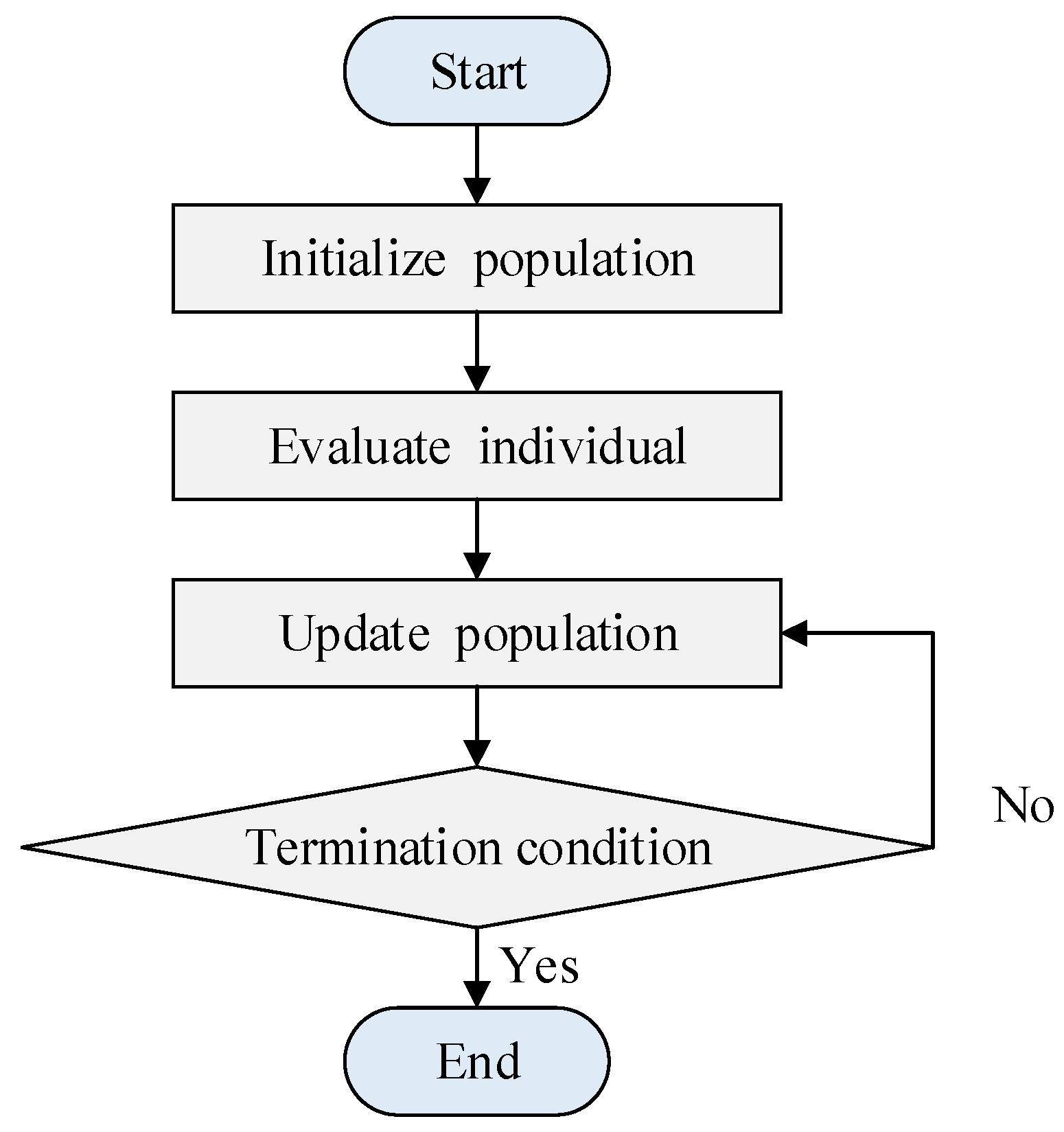
Evolutionary algorithms (EAs) are derived from the process of biological evolution. The basic principle is to simulate the evolution of biological populations through multigenerational genetic variation processes to achieve environmental adaptation. Evolutionary algorithms are generally divided into four steps: (1) initializing the population; (2) calculating the fitness of each individual in the population; (3) generating the next generation of populations by means of selection, crossover, and mutation; (4) judging the termination condition, and if it is satisfied, terminating the evolutionary algorithm; otherwise, return to step (2) (as shown in 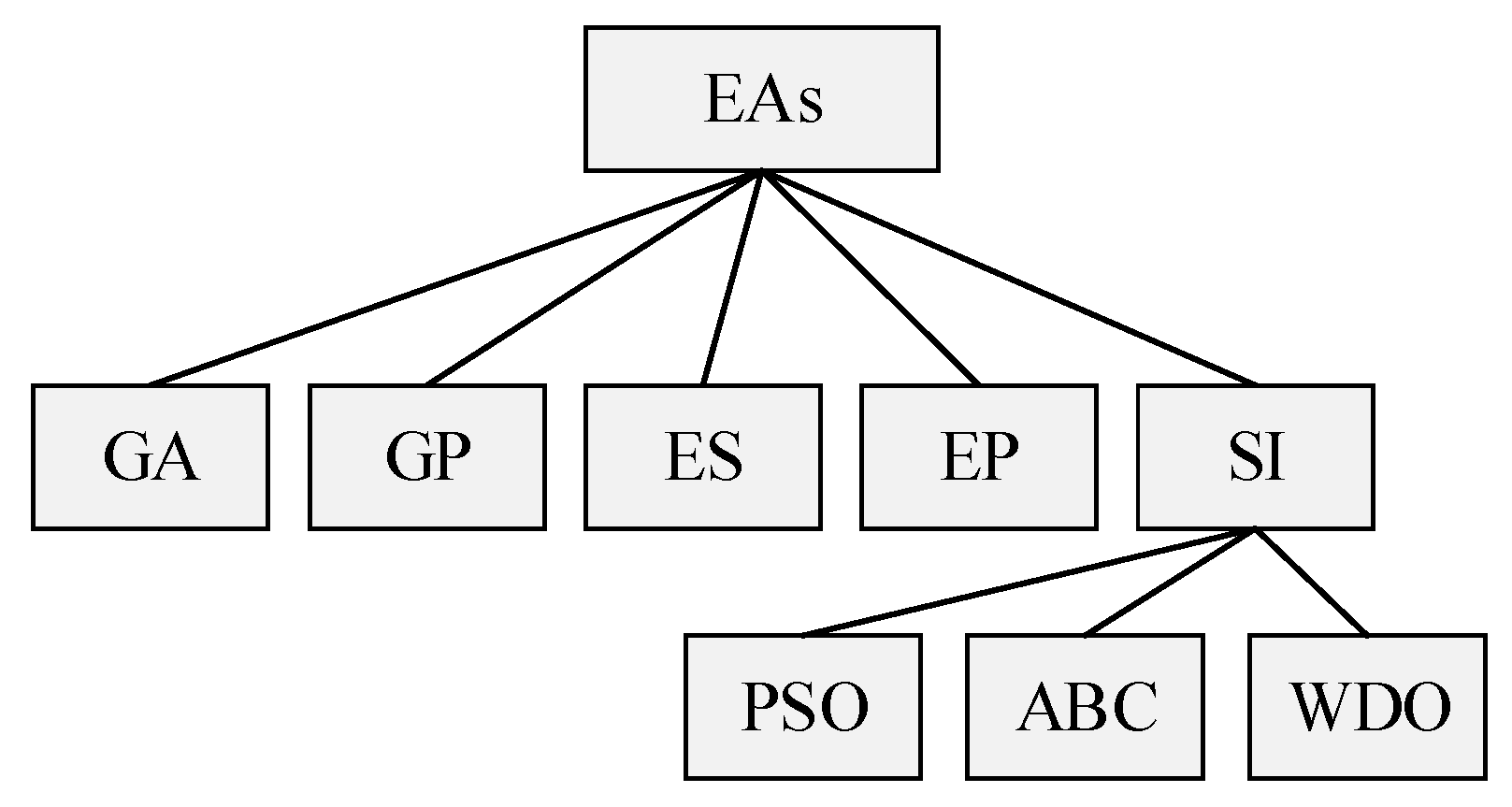Figure 1). Evolutionary algorithms include four typical methods: the genetic algorithm (GA) [6,7], genetic programming (GP) [8], evolution strategy (ES) [9] and evolutionary programming (EP) [10]. Swarm intelligence (SI) algorithms are also a special type of EA and can be defined as the collective behavior of decentralized and self-organized swarms. SI algorithms include particle swarm optimization (PSO) [11], ant colony optimization [12], and the artificial bee colony (ABC) algorithm [13] (Figure 2). Other recently proposed evolutionary techniques include wind driven optimization (WDO) [14]; invasive weed optimization (IWO) [15,16] and the covariance matrix adaptive evolution strategy (CMA-ES) [17,18].

Due to their intrinsic parallelism and powerful global search capability, EAs have emerged as viable candidates for global optimization problems, and a large number of antenna design problems have been addressed in the literature in recent years by using EAs. EAs can be real or binary-coded. Real-coded EAs are commonly used in antenna structure optimization design problems based on size or shape. This type of design can adjust the size or shape parameters of the antenna structure by an optimization algorithm based on the specified initial configuration to achieve the given single or multiple antenna performance indexes. In [19], the researchers used a combination of GA and full-wave EM tools to design a Sierpinski gasket fractal microstrip antenna. A novel coplanar waveguide fed planar monopole antenna for multiband operation was designed using a PSO algorithm in conjunction with the MOM method in [20]. Moreover, many researchers have proposed improved optimization algorithms for antenna design. For example, S. Baskar et al. [21] proposed a comprehensive learning PSO (CLPSO) algorithm, combined with the SuperNEC EM analysis toolkit to optimize the array element spacing and unit length of the Yagi–Uda antennas. Y. Sato et al. [22] proposed an adaptive GA to realize the rapid design of the meander line antenna structure. D. Ding et al. [23] proposed a modified multi-objective evolutionary algorithm based on decomposition to design a quad-band double-sided bow-tie antenna. In addition, in binary-coded EAs, each individual is encoded as a binary string, and the population is updated by crossover, mutation and a selection operator, which is well suited for discrete antenna topology optimization problems. Compared with size optimization and shape optimization, topology optimization can automatically generate “holes” in the design domain, thereby evolving the topology configuration of the structure and weakening the dependence of the entire design process on the initial configuration. In [24], the binary coded GA was applied to linear and planar array synthesis with arbitrary radiation patterns. In [25], a multi-objective evolutionary algorithm based on decomposition combined with enhanced genetic operators (MOEA/D-GO) was used to design a fragment-type MIMO dual antenna with a high isolation structure. In [26], an improved binary particle swarm optimization (BPSO) algorithm was used to design multiband or multitrap ultrawideband fragment-type antennas.

2.2. Surrogate Models

To accurately compute the antenna performance, a high-fidelity EM simulation is often required. However, it is computationally intensive to perform an EM simulation for a candidate solution, which poses a great challenge on rapid antenna design [27]. Moreover, the actual antenna design problem is mostly a multi-objective optimization problem (MOP). The use of multi-objective evolutionary algorithms (MOEAs) has led to a sharp increase in the number of evaluations of the objective function, which greatly increases the time cost of antenna optimization design, making it possible for a multi-objective optimization design to take days or even weeks to complete. Therefore, it is worthwhile improving the optimization speed at the cost of small degradation of the calculation accuracy.

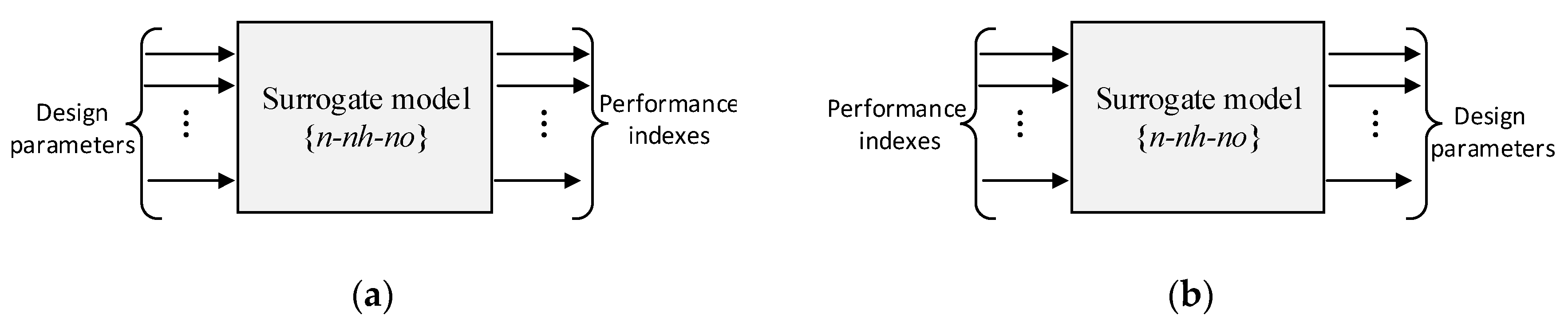
Fortunately, surrogate model techniques [28,29,30,31,32,33,34,35,36,37,38,39,40,41] have been proven to effectively avoid the huge computational cost of the EM-driven process. The use of surrogate models has been a recurrent approach adopted by the evolutionary computational community to reduce the fitness function evaluations required to produce acceptable results. The surrogate model does not address how EM simulation evaluates antenna performance. It captures the relationship between the relevant information of the input and output variables and simulates the behavior of complex systems based on a set of collected examples. The surrogate model is designed to form a black box that can be mapped between the antenna design parameters and its performance indicators (e.g., return loss, gain, and efficiency). The antenna analysis model aims to construct a mapping relationship between design parameters and performance indexes, while the antenna synthesis model is the mapping relationship between performance indexes and design parameters. The antenna synthesis model and analysis model are shown in Figure 3a,b, respectively.

The principal surrogate model techniques applied to antenna optimization problems are the kriging models [28], the support vector machines (SVMs) [29], the Gaussian processes [30] and the artificial neural networks (ANNs) [31]. The techniques can be divided into direct fitness replacement (DFR) methods and indirect fitness replacement (IFR) methods [32]. In the former group, the approximated fitness replaces the original fitness during the entire course of the EA process, while in the latter group, some, but not all processes (e.g., population initialization or EA operators) use the approximated fitness. Kriging is a spatial prediction method that belongs to the group of geostatistical methods. It is based on minimizing the mean squared error, and it describes the spatial and temporal correlation among the values of an attribute. In [33,34], S. Koziel et al. used the low-fidelity sampling points of the coarse network to construct the kriging surrogate model and then used the spatial mapping method to correct the kriging model to realize the ultrawideband (UWB) single-cone antenna and fast multitarget design of the plane quasi-Yagi antenna. On this basis, they proposed constructing a cooperative kriging (co-kriging) model by adding a limited number of high-fidelity EM response data in the iterative optimization process, thus effectively improving the prediction accuracy of the surrogate model. SVM draws inspiration from statistical learning theory and is a set of related supervised learning methods that analyzes data and recognizes patterns. SVM constructs a hyperplane or a set of hyperplanes in a high-dimensional space that can be used for classification, regression, or other tasks. In [35], the SVM is used as a surrogate model to design rectangular patch antennas and rectangular patch antenna arrays. 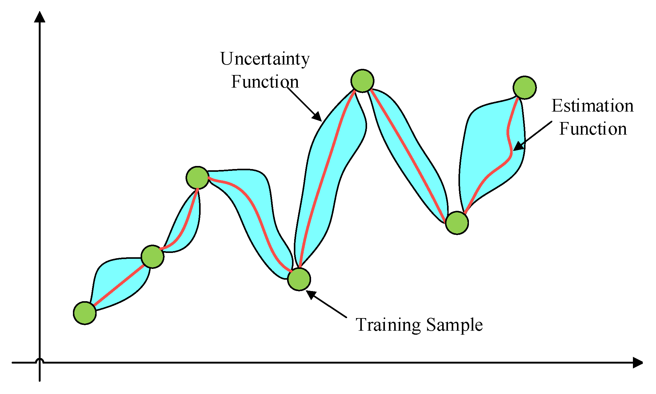The GP method is derived from the kriging model [36], which is capable of building the surrogate model while providing the approximation error (i.e., a value of uncertainty/confidentiality) of the predictions over the whole input space without the need for testing samples. A GP is completely specified by its estimation function and uncertainty function (as shown in Figure 4). The estimation function gives the expectation of the process, and the uncertainty function defines the covariance between the output random variables. Once the estimation and uncertainty functions are defined, GP can be handled following rules of probability as applied to multivariate Gaussian distributions.

In [37], the researchers constructed a gradient-enhanced GP-based surrogate model by exploiting gradient information from adjoint simulations to reduce the number of training sample points, and the method was used to design dielectric resonators and UWB antennas. ANNs are based on a nonlinear parametric model that can provide a ‘universal’ approximation capability for emulating the functions describing the behavior of complex systems. The definition of an ANN requires two steps: (i) the selection of the ANN architecture and (ii) its training. As a substitute for the fine model with high computational burden, ANN technology is rapidly developing in antenna design problems [38,39,40,41]. In [38], a radial basis function neural network (RBFNN) was used to estimate the directivity of a uniform linear array of collinear short dipoles and parallel short dipoles. In [39], multilayer perceptron NN (MLP-NN)-based model and differential evolution algorithm are used to optimize performance index for reconfigurable antenna. In [40], the BP algorithm-based MLP-NN as antenna analysis model is combined with the particle swarm optimization (PSO) algorithm to form a design program for making a custom fractal antenna, and a Sierpinski gasket and Koch monopole antennas were taken as the candidate antennas to verify effectiveness of the developed approach. In [41], a sparsely connected neural network optimized (SC-BPNN) by HPSO algorithm was proposed and used as a surrogate model to participate in planar miniaturized multi-band antenna design. The proposed SC-BPNN has a high prediction accuracy and a simplified network structure, but the comparison experiment results show that the method has a larger time cost compared with other BPNN-based surrogate models as the HPSO optimization process is time consuming.

3. Research Motivation

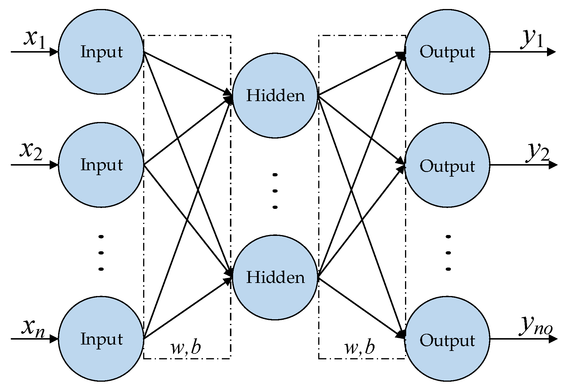
BPNN are based on a non-linear parametric model which is able to provide an ’universal’ approximation capability for emulating the functions describing the behavior of complex systems. In theory, a multi-layer BPNN can approximate any complex nonlinear function [42]. However, in order to avoid excessive computational complexity, a three-layer BPNN as shown in Figure 5 is usually chosen. The neurons between adjacent layers are connected in a fully connected manner, and each connection corresponds to a weight value. The output layer obtains the error between the actual output and the expected result, and then updates the weight in direction of the largest gradient according to the gradient descent algorithm. Finally, the error is forwarded to the input layer once to complete the update of the weight. The quadratic cost function C₀ of conventional BPNN and the weight and bias update formula are as follows

$$C_0(w,b)=\frac{1}{2n}{{\displaystyle {\sum }_{x_i}\Vert y_k\left(x_i\right)-Y_k\left(x_i\right)\Vert }}^2$$

(1)

$$\begin{array}{l}w\to w^{\prime }=w-\eta \frac{\partial C_0}{\partial w}\\ b\to b^{\prime }=b-\eta \frac{\partial C_0}{\partial b}\end{array}$$

(2)

where x_i is the input of ith neuron and represents an antenna structure design variable; n is the number of input neurons; $y_k$ and $Y_k$ is the output of kth neuron and expected result respectively; $no$ is the number of output neurons; $w$ denotes the mapping relationship between adjacent nodes; $w^{\prime }$ denote the updated link weight; $b$ and $b^{\prime }$ denote the biases between adjacent nodes and the updated biases, respectively; $\eta$ is a learning factor. The BPNN surrogate model is designed to construct a black box that can be mapped between the antenna design parameters and its performance indicators.

Since BPNN has the ability to approximate nonlinear maps well and can simulate nonlinear functions with an arbitrary precision, it is very suitable to replace the EM tools in traditional antenna designs. However, the traditional BPNN has some shortcomings, which makes the construction of the surrogate model too expensive and the prediction accuracy not high. First, the network structure of the traditional BPNN can only adjust the number of neurons in the input layer, the hidden layer, and the output layer, and cannot fine-tune the links between the layers, resulting in a network structure that is not compact enough and wastes computing resources. Second, the BPNN generally has over-fitting phenomenon, mainly due to too few training sample points or too complex network structures, resulting in network learning noise data in training sets. Therefore, a simple, compact BPNN is designed to reflect the performance of a multi-parameter antenna structure in real time.

The major innovation contributions as summarized as follows: (1) A new l₁-BPNN surrogate model is proposed, and l₁ optimization [43] is used to automatically determine all mapping parameters and states in the BPNN model to achieve the most appropriate and compact structure of the surrogate model; (2) Based on the proposed l₁-BPNN model, a computationally efficient analysis strategy is established for predicting the performance indexes of the particular antenna structure, and then a fast multi-objective optimization framework for multiparameter structures is formed.

4. Our Approach

4.1. l₁-BPNN Model

Since BPNN uses the gradient descent algorithm, the stability of the network requires little learning efficiency, resulting in a slower network convergence speed. At the same time, the multi-layer network is often interfered by the local optimal solution, and whether the learning process falls into the local optimal solution is closely related to the initial parameters (weights w and thresholds b) of the network [44]. In addition, the network structure will have an impact on the overall learning ability. Too complex network structure can cause the learning process to be too slow and easily lead to overfitting phenomenon [41]. On the contrary, too simple network structure may lead to insufficient learning ability.

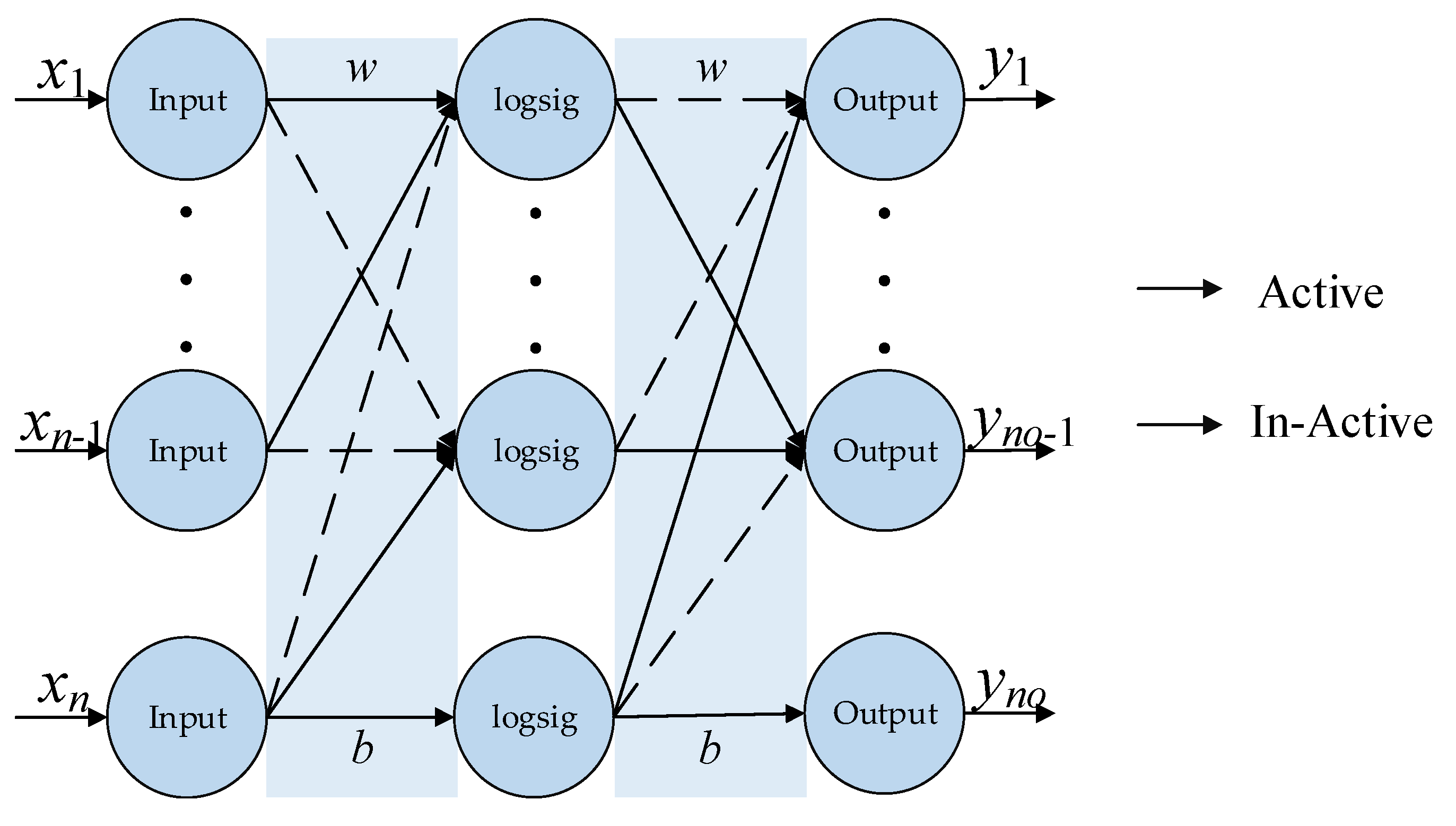
Therefore, we propose a new formulation using l₁ optimization to automatically determine network structure and connection parameter. The l₁ optimization has the distinctive property for feature selection within the training process. In the l₁ optimization process, the optimization goal is to maximize g, and at the end of l₁ optimization, some weights in the neural networks are zeros while others remain nonzero. Zero weights mean that the corresponding parts of the mapping can be ignored and deleted. The cost function of l₁-BPNN model is expressed as follows

$$C=C_0+\frac{\lambda }{N}{\displaystyle {\sum }_w\left|w\right|}$$

(3)

$$g=\frac{1}{1+C}$$

(4)

where C₀ is used to determine the updated direction and updated size of the connection parameters; C is the updated cost function and connection parameter is updated as shown in formula (5); N is the size of the training set, and λ > 0 is the normalized parameter; sgn() is used to return the sign of the parameter.

$$\begin{array}{c}w\to w^{\prime }=w-\eta \frac{\partial C_0}{\partial w}-\frac{\eta \lambda }{N}\mathrm{sgn}(w)\\ b\to b^{\prime }=b-\eta \frac{\partial C_0}{\partial b}\end{array}$$

(5)

l₁ optimization increases the punishment for large weights, tending to small network weights, so that a small number of important connection parameters in the network are preserved, while relatively less important connections will be close to 0, which is inactive, eventually making the network structure sparse. An l₁-BPNN model is given in Figure 6, where logsig($\cdot$) is the most commonly used S-type transfer function for hidden layers, and defined as

$$\log \mathrm{sig}\left(x_i\right)=\frac{1}{1+e^{-x_i}},x_i\in \Re .$$

(6)

Compared with the traditional BPNN model with fixed mapping structure, the l₁-BPNN model can adjust the mapping structure automatically in addition to the number of neurons to achieve the most suitable and compact structure of the surrogate model.

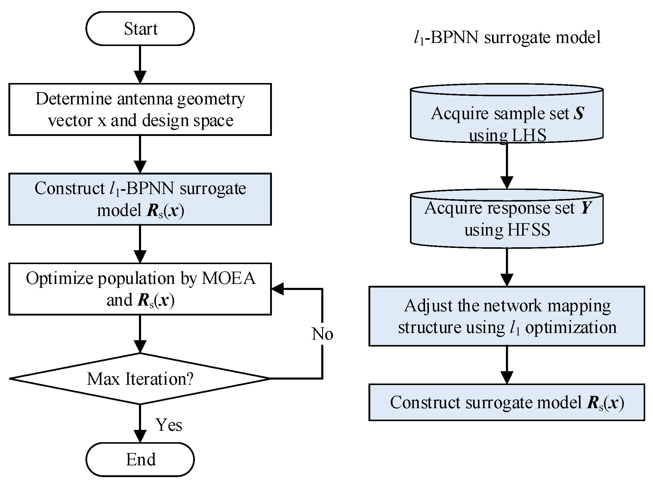
4.2. Fast Multi-Objective Antenna Optimization Framework Combining MOEAs and l₁-BPNN Surrogate Model

In this section, we use the l₁-BPNN surrogate model discussed in the previous section, rather than conventionally time-consuming EM simulations, to evaluate the antenna performance. The first step in building a surrogate model is to use Latin hypercube sampling (LHS) [45,46] to obtain a uniformly distributed and representative sample set S = [s₁,s₂,…,s_q]^T, and to import those sample sets S into the EM tool to achieve high-accuracy response set Y. The quality of S and Y is directly related to the generalization ability of the surrogate model, but the process is the most time consuming in the overall surrogate model construction. Then S and Y will be used as input layer data and output layer data to construct antenna surrogate model R_s(x), respectively. The l₁ optimization method automatically adjusts the network mapping structure in this process. Thus, the whole multi-objective optimization framework is summarized as follows:

• Predefine the design space;
• Determine the number of neurons in each layer of NN and the antenna geometry vector x;
• Sample design space using LHS and acquire the response set Y;
• Adjust the network mapping structure by l₁ optimization;
• Construct an l₁-BPNN surrogate model R_s(x);
• Optimize the population by MOEA with an l₁-BPNN surrogate model;
• If termination condition is not satisfied then go to 6; else end optimization.

The flowchart of MOEA with an l₁-BPNN surrogate model is shown in Figure 7. It is expected that our approach will greatly reduce the computational cost of the antenna optimization process and meanwhile speed up the convergence.

5. Verification Case Study and Discussions

This section will give an application example of a miniaturized planar triple-band antenna design to further illustrate the advantages of the fast multi-objective antenna optimization framework constructed by l₁-BPNN model.

5.1. l₁-BPNN Antenna Surrogate Model

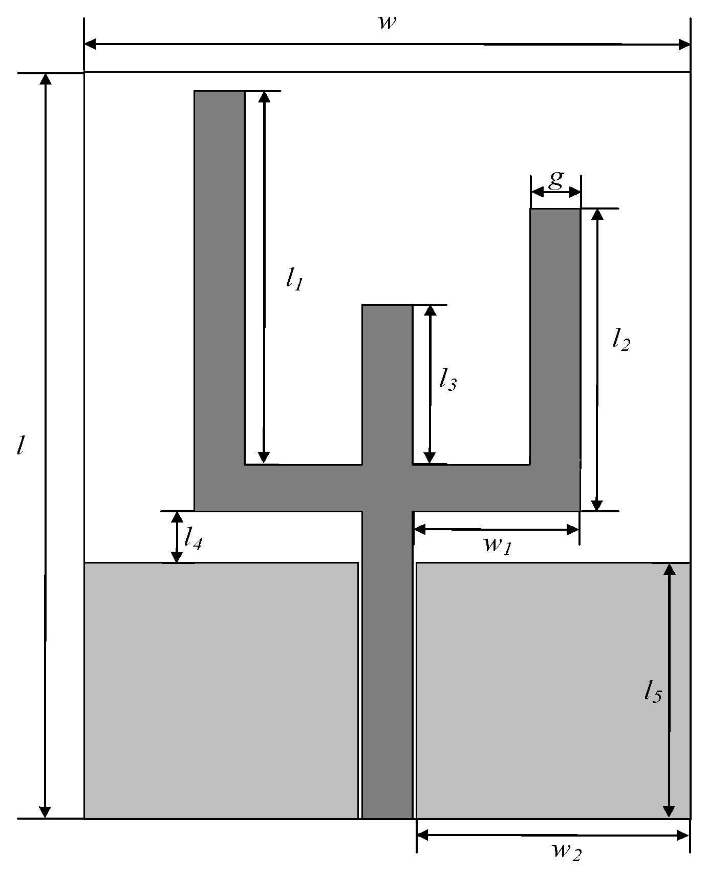
The initial structure of the planar monopole antenna is shown in Figure 8. This antenna is formed by a fork-shaped radiator and a rectangle ground plane, which produces different resonant frequency bands to satisfy multiband applications. The antenna is printed on a Rogers RO4003(tm) substrate with a thickness of 0.5 mm, permittivity of 3.55, and loss tangent of 0.0027. Design variables are $x={[l{l}_1{l}_2{l}_3{l}_4{l}_{5}w{w}_1{w}_{2}g]}^T$ and initial ranges are given in

Table 1. Initial Ranges of Design Parameters.

Parameter	l	l1	l2	l3	l4
Range	[36, 40]	[16, 19]	[10, 12.5]	[8.5, 10.5]	[2.8, 3.9]
Parameter	l5	w	w1	w2	g
Range	[9.5, 11.5]	[19, 24]	[6.5, 8.3]	[8.7, 11.2]	[1.8, 2.1]

(Units: mm).

A high-precision surrogate model means that a large number of training sets and response sets need to be acquired, which makes the computational cost increase dramatically. The surrogate model we want to construct is low-cost and can respond to trends in performance indexes. Therefore, the LHS is introduced to sample design space and obtain a representative sample set S including 200 sample points. Next, we acquire the high fidelity response set Y of sampling points by using EM simulation software HFSS, S and Y are used as input layer data and output layer data to construct l₁-BPNN surrogate model, respectively. As for the determination of the number of hidden layer nodes, although there are some empirical formulas for reference, there is no mature theory as a guide. In order to ensure the stability of the network, experimental tests are used to determine the number of hidden layer nodes. The node test interval is taken as [10, 20]. Then S and Y will be used as input layer data and output layer data to construct antenna surrogate model R_s(x), respectively. The l₁ optimization method automatically adjusts the network mapping structure in this process.

Table 2. Comparison of Fitness Values for Predicting the S₁₁ Values.

nh	l1-BPNN		Conventional BPNN		PSO-BPNN
	Fitness Values	Number of Links	Fitness Values	Number of Links	Fitness Values	Number of Links
10	0.9318	154	0.8892	275	0.9190	275
11	0.9435	186	0.8781	301	0.8879	301
12	0.9419	235	0.8971	327	0.9074	327
13	0.9457	254	0.9056	353	0.9313	353
14	0.9478	210	0.9022	379	0.9147	379
15	0.9324	248	0.9130	405	0.9203	405
16	0.9299	259	0.8975	431	0.9138	431
17	0.9365	282	0.9087	457	0.9312	457
18	0.9528	311	0.8909	483	0.9383	483
19	0.9531	367	0.8925	509	0.9205	509
20	0.9501	389	0.9053	535	0.9226	535

shows the fitness values and the number of network mapping of the three models (the proposed l₁-BPNN over the traditional BPNN [40], the BPNN optimized by PSO (PSO-BPNN) [47]). From Table 2, we have the observation that the l₁-BPNN generally has better fitness values and a simpler network mapping structure than other models. Through this experiment, we choose the network mapping structure when the number of hidden nodes is 19, and its connection parameters only account for 72% of other models.

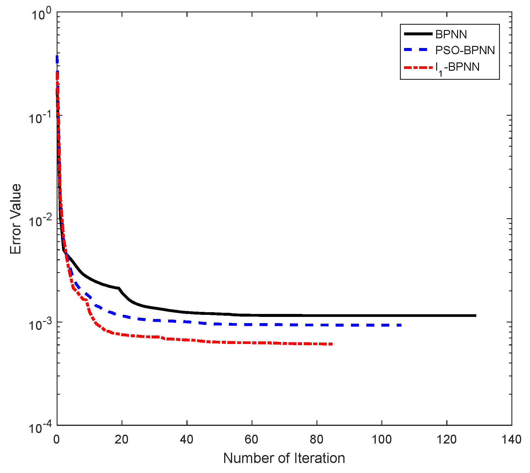
Figure 9 shows the error value curves of the three models during training process. It can be observed that the number of iterations and the training error of the proposed model are smaller than the other two models, indicating that l₁-BPNN has better convergence performance and training accuracy.

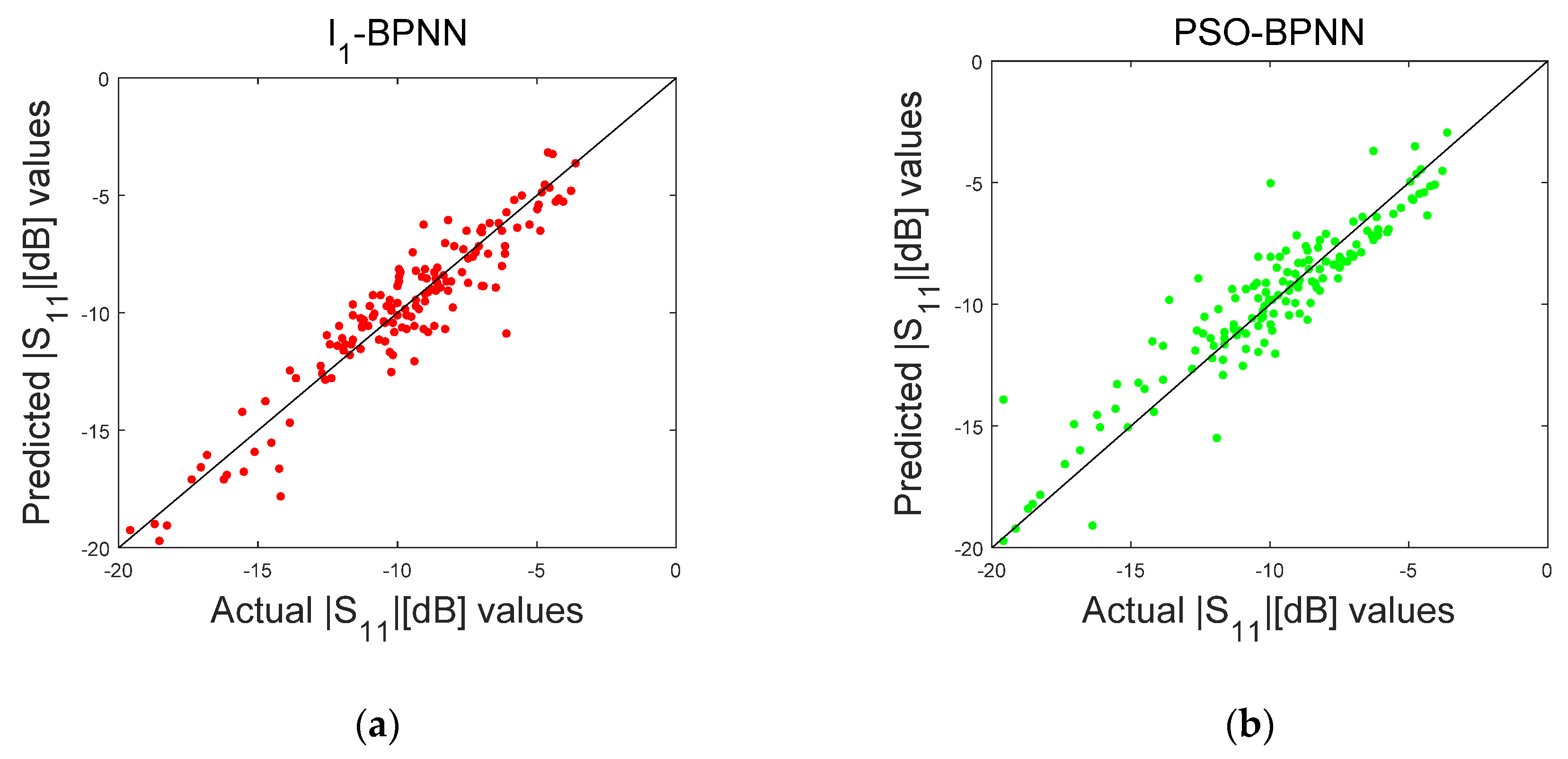
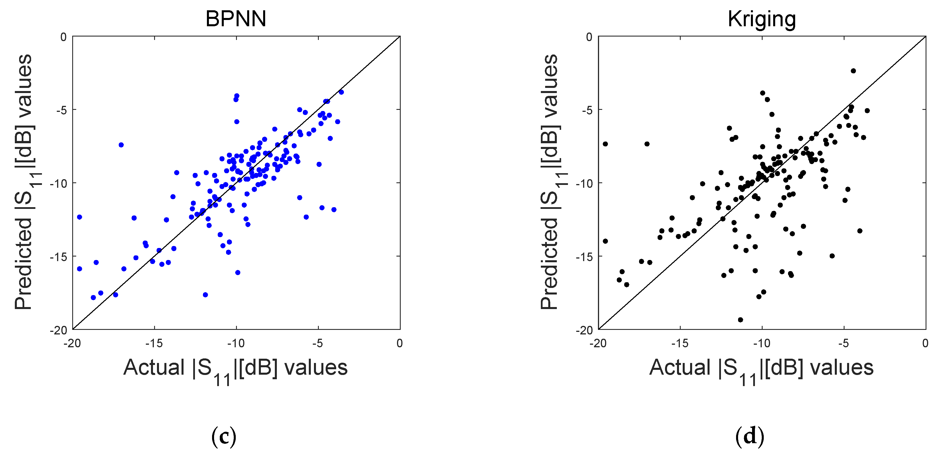
In addition, Figure 10 shows a comparison of the predictions of Kriging [33], traditional BPNN [40], PSO-BPNN [47], and l₁-BPNN with the HFSS response results. Compared to Figure 10b–d, Figure 10a is more concentrated, indicating that the predicted structure of l₁-BPNN is closer to the HSFF response.

Table 3. Computational Time of Various Surrogate Models and HFSS Simulations.

Model	HFSS	Kriging	BPNN	PSO-BPNN	l1-BPNN
Total time (s)	587.82	1.92	0.36	0.28	0.26
Average time(s)	58.78	0.192	0.036	0.028	0.026

clearly lists the time costs of different surrogate models and EM simulations. It is observed that the surrogate model is generally less time consuming.

In summary, our proposed l₁-BPNN model can be used for performance prediction efficiently instead of EM simulation software and achieve a fast multi-objective optimization with the help of MOEAs for a predefined antenna geometry.

5.2. Pareto-Optimal Designs of a Planar Miniaturized Multiband Antenna

In this section, the MOEA/D [48] and l₁-BPNN model are combined to achieve fast multi-objective optimization of the planar antenna geometry presented in Figure 9. Two design goals are (i) the values of S₁₁ are lower than −10dB within the frequency bands of 2.40–2.60 GHz, 3.30–3.80 GHz, 5.00–5.85 GHz, covering the entire WLAN2.4/5.2/5.8 GHz and WiMAX3.5 GHz applications (objective F₁); (ii) the size of the antenna structure is reduced to satisfy the need for antenna miniaturization in portable electric devices (objective F₂). The objective function of F₁ is specified as

$$F_1=\frac{1}{N}{\displaystyle \sum _{i=1}^{n}Q(f_i)}$$

(7)

$$Q(f_i)=\{\begin{array}{ll}\left|S_{11}(f_i)\right|& \left|S_{11}(f_i)\right|>-10\\ -10& \left|S_{11}(f_i)\right|\le -10\end{array}$$

(8)

where f_i is the ith sampling frequency point within the given bands of operation; $S_{11}(f_i)$ is the reflection coefficient of sampling point f_i; N is the number of sampling frequency points. The objective function of F₂ can be defined as

$$F_2=w\times l$$

(9)

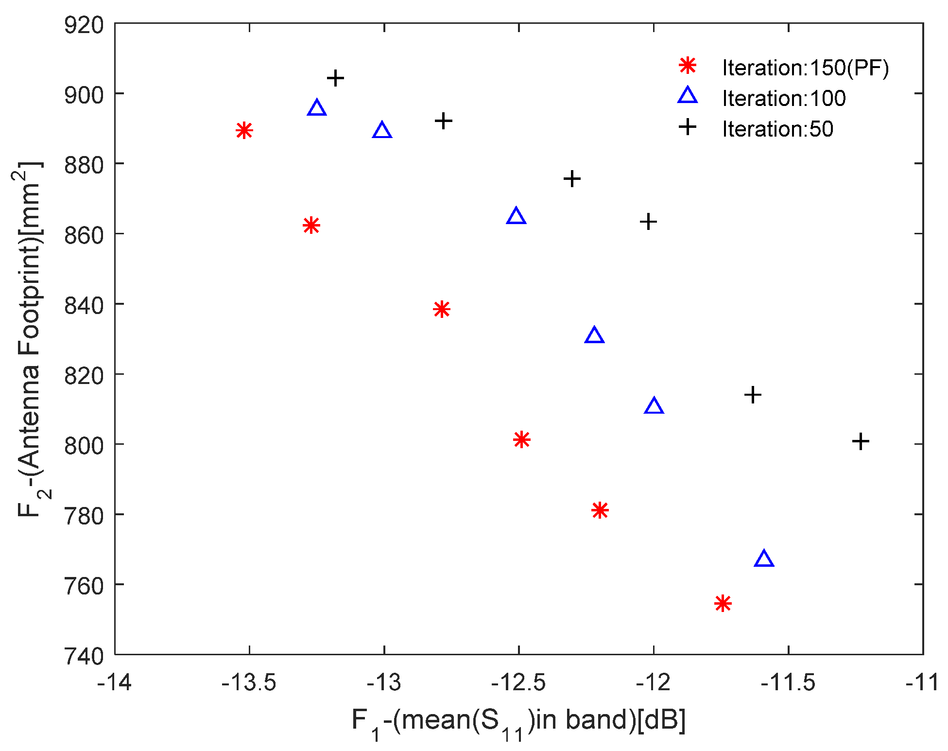
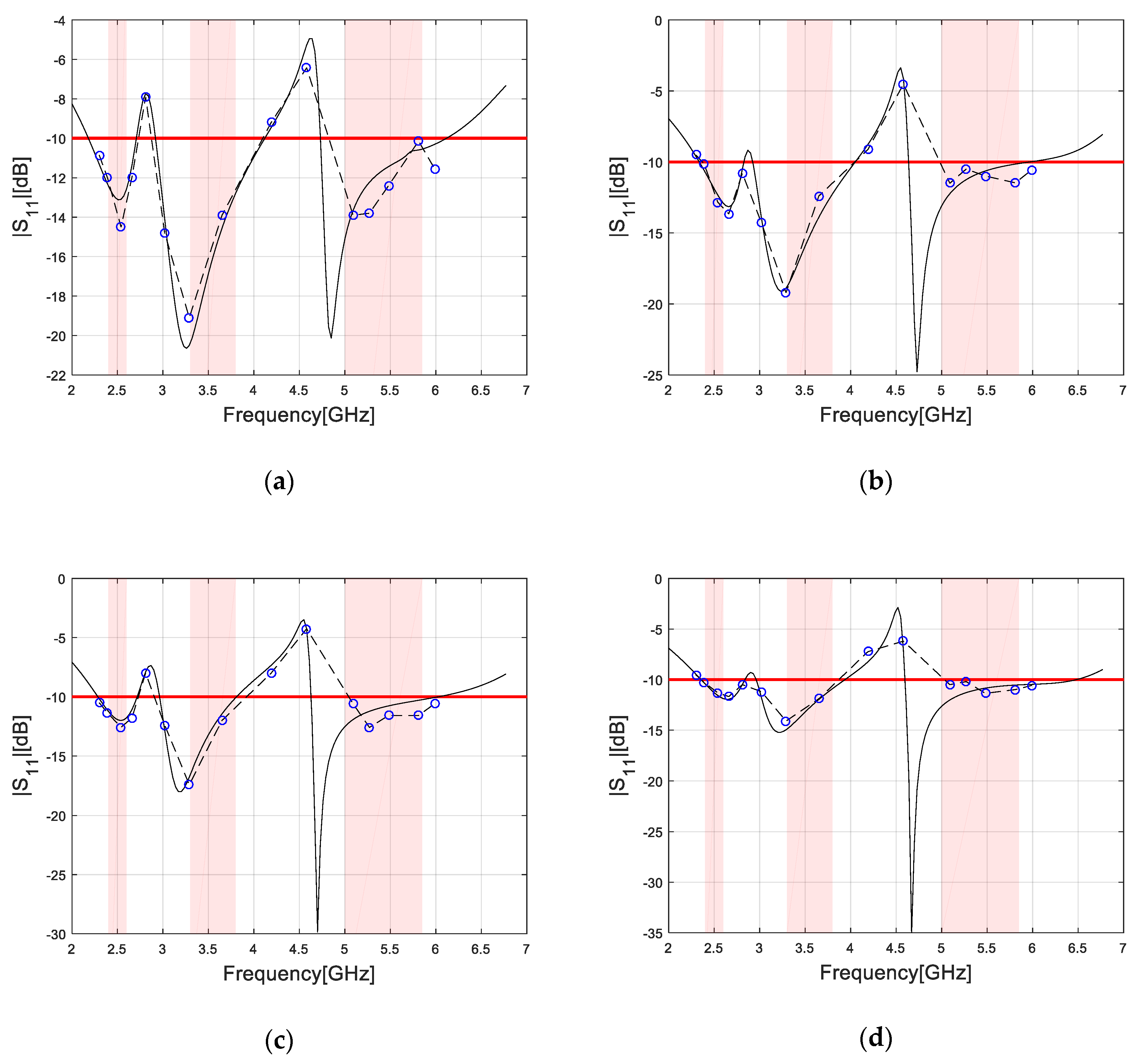
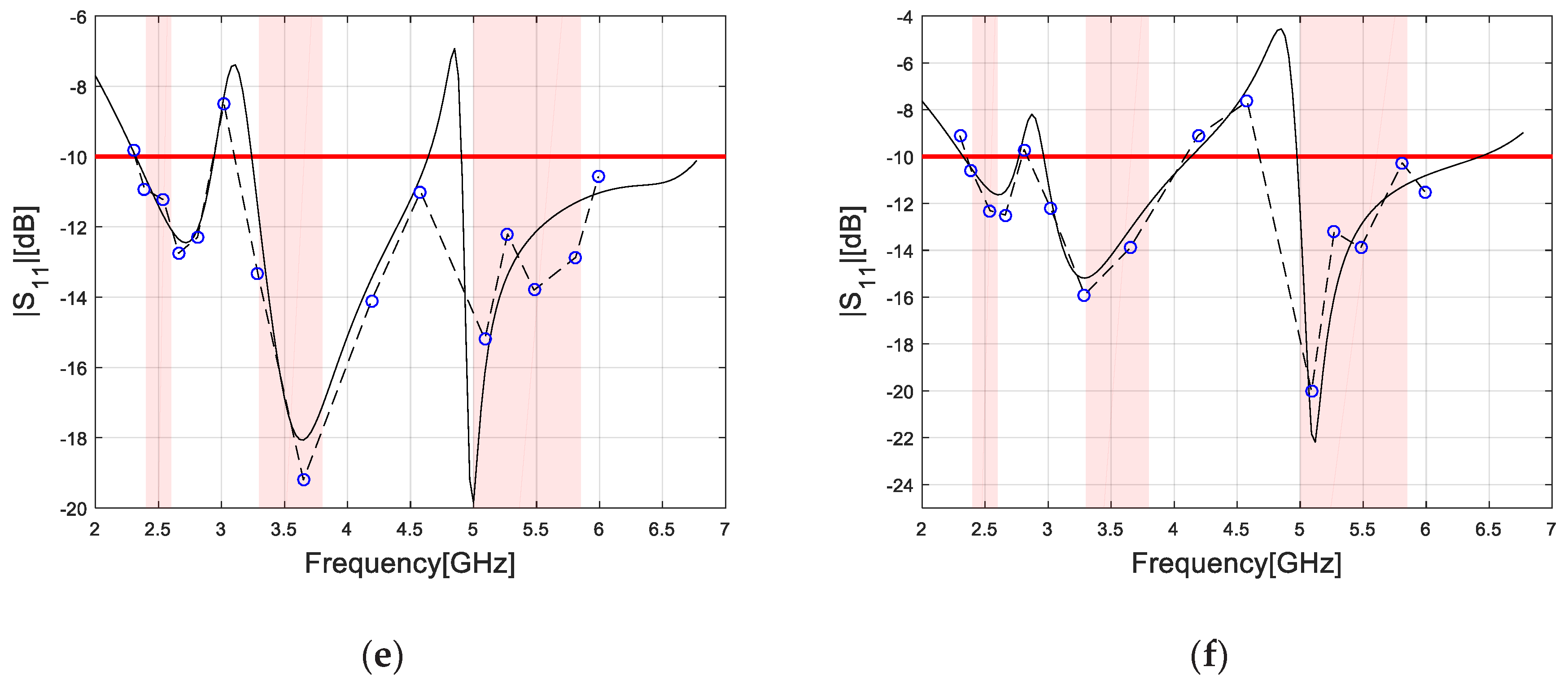
The parameters of MOEA/D [48] are set as follows: the number of population is 100, and the maximum number of iterations is 150. Figure 11 displays the representation of the Pareto set of the optimized antenna at different iterations. It can be observed that as the number of iterations increases, the objective function becomes closer to a smaller size and a lower S₁₁ value. The detailed antenna designs are given in

Table 4. Planar Multiband Antenna: Selected Pareto-Optimal Designs.

Design	${\mathit{x}}^{(1)}$	${\mathit{x}}^{(2)}$	${\mathit{x}}^{(3)}$	${\mathit{x}}^{(4)}$	${\mathit{x}}^{(5)}$	${\mathit{x}}^{(6)}$
$F_1[dB]$	−13.52	−13.27	−12.78	−12.49	−12.20	−11.74
$F_2[m{m}^2]$	889.35	862.14	838.10	801.27	781.19	754.46
l	38.4	38.7	39.0	38.0	39.1	37.9
l1	17.5	18.3	17.1	17.8	16.6	17.5
l2	12.4	11.2	12.2	11.4	11.9	11.7
l3	10.2	9.9	9.6	10.3	9.4	10.2
l4	3.3	3.2	3.3	3.1	3.3	3.0
l5	9.7	9.6	9.9	10.1	10.4	9.8
w	23.2	22.3	21.5	21.1	19.9	19.7
w1	6.5	7.1	7.3	7.2	7.4	7.5
w2	10.4	9.4	10.2	9.6	9.5	9.0
g	2.0	1.9	1.9	2.0	1.9	1.9

. Furthermore, Figure 12 demonstrates the good fitting ability of the l₁-BPNN model. The HFSS simulation curve of the Pareto-optimal designs well matches the l₁-BPNN prediction values. In addition, S₁₁ curves of all designs cover the target frequency band (red shadow) to meet the preset application requirements. Figure 12 shows how close the predicted value of the surrogate model we constructed is to the EM curve. Additionally, it is observed that the S₁₁ curve is lower than −10 dB within the three frequency bands of 2.33–2.66 GHz, 3.05–3.80 GHz, and 5.06–5.96 GHz, simultaneously satisfying the WLAN and WiMAX applications.

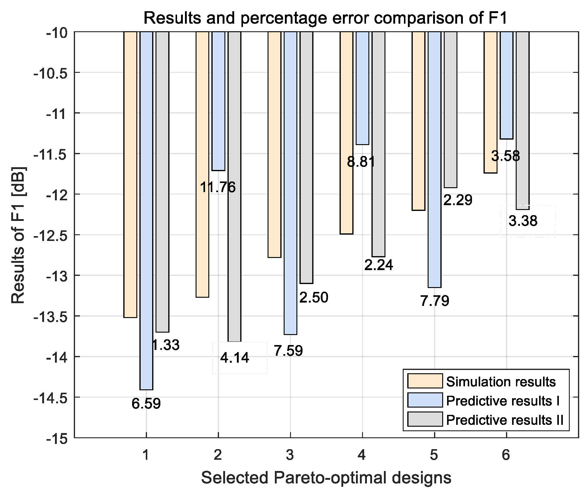
In order to verify the feasibility and validity of l₁-BPNN model, the results of fitness F₁ and percentage error for those selected Pareto-optimal designs, which are calculated by different approaches, are listed in

Table 5. Comparison of Fitness Values F1 of Selected Pareto-Optimal Designs Obtained by Surrogate Model and HFSS.

Design	x(1)	x(2)	x(3)	x(4)	x(5)	x(6)
Simulation results	−13.52	−13.27	−12.78	−12.49	−12.20	−11.74
Predictive results I	−14.41	−11.71	−13.75	−11.39	−13.15	−11.32
Predictive results II	−13.70	−13.82	−13.10	−12.77	−11.92	−12.19
Error rate I (%)	6.59	11.76	7.59	8.81	7.79	3.58
Error rate II (%)	1.33	4.14	2.50	2.24	2.29	3.38

, and Figure 13 shows an error comparison histogram between simulation results and prediction results in Table 5. The predictive results 1 and predictive results 2 are given by traditional BPNN and l₁-BPNN surrogate model strategy, respectively. The minimum error percentages are 3.58% and 1.33% for prediction results 1 (with an average error of 7.69%) and prediction results 2 (with an average error of 2.65%), respectively. Therefore, our proposed l₁-BPNN is meaningfully better than the conventional BPNN with an acceptable error rate.

Furthermore,

Table 6. Comparison of Computational Cost among Different Antenna Optimization Schemes.

Optimization Approach	Number of EM Simulations	CPU Time/h
		Total	Relative (%)
Scheme I	15,000	245.96	100
Scheme II	200	3.38	1.37
Scheme III	200	3.71	1.51
Scheme IV	200	3.11	1.26

lists the computational cost comparisons for the four antenna optimization methods. Scheme I is direct MOEA/D-based optimization without a surrogate model. Scheme II, Scheme III and Scheme IV are based on the traditional BPNN [40], SC-BPNN [41], and l₁-BPNN surrogate model, respectively. As listed in Table 6, the time cost of Scheme IV represents only 1.26% of scheme I, scheme II is approximately 1.37% of the time cost of scheme I, and scheme III is approximately 1.51% of the time cost of scheme I. 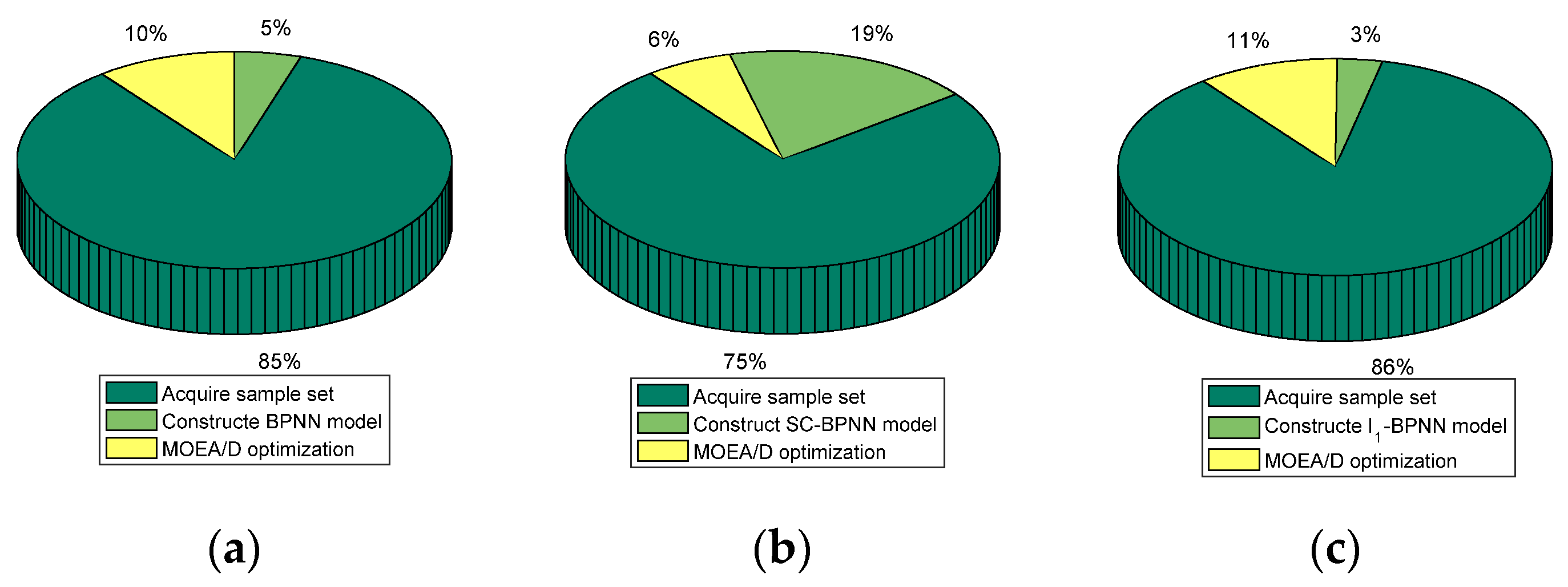Figure 14 shows the time-consuming ratio of each part of the multi-objective optimization method using the different surrogate models. As shown in Figure 14b, since SC-BPNN requires a time-consuming HPSO optimization process, its model construction time cost is the largest among these three surrogate-assisted methods. On the contrary, as shown in Figure 14c, since our proposed model has a simplified network structure and requires fewer training times, its model construction time cost is the smallest among these three surrogate-assisted methods.

6. Conclusions

An improved BPNN surrogate model is developed in this paper to applied low-cost multi-objective multiparameter antenna optimization. To overcome the shortcomings of the traditional BPNN, an l₁-BPNN model is proposed. Some modifications are given for better network performance, including automatically adjusting the network mapping structure by l₁ optimization. Compared with other existing BPNN-based surrogate models, the proposed l₁-BPNN model has smaller construction cost, better convergence performance, and prediction accuracy. Then, by integrating the l₁-BPNN surrogate model with MOEAs, a low-cost antenna design method is established, which can quickly realize the optimal design of multi-objective and multi-parameter antenna structures. This technique has been illustrated using a planar antenna structure. Comparison with the previously published surrogate model scheme indicates significant savings of the overall optimization cost that can be achieved with our l₁ optimization method.

Although the results from this study are very encouraging, further research will be conducted to address several issues. First, the connection parameters are decremented to zero at a constant speed during l₁ optimization. When the absolute value of a weight is large, the speed of optimization is too slow. So, we intend to improve the l₁ algorithm so that the weight reduction speed is related to the absolute value of the weight to improve the optimization efficiency. Second, the proposed method is a direct fitness surrogate method, which cannot be updated in the EA process. Therefore, we want to study the dynamically updated BPNN surrogate model, which aims to improve the utilization of EM data and further reduce its construction cost.

References

- Milligan, T.A. Modern Antenna Design, 2nd ed.; John Wiley & Sons: Hoboken, NJ, USA, 2005. [Google Scholar]
- Fujimoto, K. Mobile Antenna Systems Handbook, 3rd ed.; Artech House: Norwood, MA, USA, 2008. [Google Scholar]
- Dziunikowski, W. Multiple-Input Multiple-Output (MIMO) Antenna Systems. In Adaptive Antenna Arrays: Signals and Communication Technology; Chandran, S., Ed.; Springer: Berlin, Germany, 2004; pp. 259–273. [Google Scholar]
- McGrath, D.; Pyati, V. Phased array antenna analysis with the hybrid finite element method. IEEE Trans. Antennas Propag. 1994, 42, 1625–1630. [Google Scholar] [CrossRef]
- Choi, W.-S.; Sarkar, T. Phase-Only Adaptive Processing Based on a Direct Data Domain Least Squares Approach Using the Conjugate Gradient Method. IEEE Trans. Antennas Propag. 2004, 52, 3265–3272. [Google Scholar] [CrossRef]
- Goldberg, D.E. Genetic Algorithms in Search, Optimization and Machine Learning; Addison-Wesley: New York, NY, USA, 1989. [Google Scholar]
- Holland, J.H. Adaptation in Natural and Artificial Systems; The University of Michigan Press: Ann Arbor, MI, USA, 1975. [Google Scholar]
- Koza, J.R.; Poli, R. Genetic Programming. In Search Methodologies; Burke, E.K., Kendall, G., Eds.; Springer: Boston, MA, USA, 2005; pp. 127–164. [Google Scholar]
- Beyer, H.-G.; Schwefel, H.-P. Evolution strategies – A comprehensive introduction. Nat. Comput. 2002, 1, 3–52. [Google Scholar] [CrossRef]
- Fogel, D.B. Evolutionary Computation: Toward a New Philosophy of Machine Intelligence; IEEE Press: Piscataway, NJ, USA, 1995. [Google Scholar]
- Kennedy, J.; Eberhart, R.C. Particle swarm optimization. In Proceedings of the 1995 IEEE International Conference on Neural Networks, Perth, Australia, 27 November–1 December 1995; pp. 1942–1948. [Google Scholar]
- Dorigo, M.; Stutzle, T. Ant Colony Optimization; The MIT Press: Cambridge, MA, USA, 2004. [Google Scholar]
- Karaboga, D.; Basturk, B. A powerful and efficient algorithm for numerical function optimization: Artificial bee colony (ABC) algorithm. J. Glob. Optim. 2007, 39, 459–471. [Google Scholar] [CrossRef]
- Bayraktar, Z.; Bossard, J.A.; Werner, D.H.; Komurcu, M. The Wind Driven Optimization Technique and its Application in Electromagnetics. IEEE Trans. Antennas Propag. 2013, 61, 2745–2757. [Google Scholar] [CrossRef]
- Zaharis, Z.D.; Lazaridis, P.I.; Cosmas, J.; Skeberis, C.; Xenos, T.D. Synthesis of a Near-Optimal High-Gain Antenna Array With Main Lobe Tilting and Null Filling Using Taguchi Initialized Invasive Weed Optimization. IEEE Trans. Broadcast. 2014, 60, 120–127. [Google Scholar] [CrossRef] [Green Version]
- Zaharis, Z.; Skeberis, C.; Xenos, T.D.; Lazaridis, P.; Cosmas, J. Design of a Novel Antenna Array Beamformer Using Neural Networks Trained by Modified Adaptive Dispersion Invasive Weed Optimization Based Data. IEEE Trans. Broadcast. 2013, 59, 455–460. [Google Scholar] [CrossRef] [Green Version]
- Boudaher, E.; Hoorfar, A. Electromagnetic design optimization using mixed-parameter and multiobjective CMA-ES. In Proceedings of the IEEE Antennas and Propagation Society International Symposium (APSURSI ’13), Orlando, FL, USA, 7–13 July 2013; pp. 406–407. [Google Scholar]
- BouDaher, E.; Hoorfar, A. Electromagnetic Optimization Using Mixed-Parameter and Multiobjective Covariance Matrix Adaptation Evolution Strategy. IEEE Trans. Antennas Propag. 2015, 63, 1712–1724. [Google Scholar] [CrossRef]
- Ghatak, R.; Poddar, D.; Mishra, R. Design of Sierpinski gasket fractal microstrip antenna using real coded genetic algorithm. IET Microwaves Antennas Propag. 2009, 3, 1133–1140. [Google Scholar] [CrossRef]
- Liu, W.-C. Design of a multiband CPW-fed monopole antenna using a particle swarm optimization approach. IEEE Trans. Antennas Propag. 2005, 53, 3273–3279. [Google Scholar]
- Baskar, S.; Alphones, A.; Suganthan, P.N.; Liang, J.J. Design of Yagi-Uda antennas using comprehensive learning particle swarm optimization. IEE Proc. Microw. Antennas Propag. 2005, 152, 340–346. [Google Scholar] [CrossRef]
- Sato, Y.; Campelo, F.; Igarashi, H. Meander Line Antenna Design Using an Adaptive Genetic Algorithm. IEEE Trans. Magn. 2013, 49, 1889–1892. [Google Scholar] [CrossRef] [Green Version]
- Ding, D.; Wang, G. Modified Multiobjective Evolutionary Algorithm Based on Decomposition for Antenna Design. IEEE Trans. Antennas Propag. 2013, 61, 5301–5307. [Google Scholar] [CrossRef]
- Marcano, D.; Duran, F. Synthesis of antenna arrays using genetic algorithms. IEEE Antennas Propag. Mag. 2000, 42, 12–20. [Google Scholar] [CrossRef]
- Ding, D.; Wang, L.; Wang, G. High-efficiency scheme and optimisation technique for design of fragment-type isolation structure between multiple-input and multiple-output antennas. IET Microw. Antennas Propag. 2015, 9, 933–939. [Google Scholar] [CrossRef]
- Dong, J.; Li, Q.; Deng, L. Design of Fragment-Type Antenna Structure Using an Improved BPSO. IEEE Trans. Antennas Propag. 2018, 66, 564–571. [Google Scholar] [CrossRef]
- John, M.; Ammann, M.J. Antenna Optimization with a Computationally Efficient Multiobjective Evolutionary Algorithm. IEEE Trans. Antennas Propag. 2009, 57, 260–263. [Google Scholar] [CrossRef]
- Sacks, J.; Mitchell, T.J.; Welch, W.J.; Wynn, H.P. Design and Analysis of Computer Experiments. Stat. Sci. 1989, 4, 409–423. [Google Scholar] [CrossRef]
- Vapnik, V.N. Statistical Learning Theory, Adaptive and Learning Systems for Signal Processing, Communications, and Control; John Wiley & Sons: New York, NY, USA, 1998. [Google Scholar]
- Rasmussen, C.; Williams, C. Gaussian Processes for Machine Learning; The MIT Press: Cambridge, MA, USA, 2008. [Google Scholar]
- Mao, J.; Mohiuddin, K.; Jain, A. Artificial neural networks: A tutorial. Computer 1996, 29, 31–44. [Google Scholar]
- Shi, L.; Rasheed, K. A Survey of Fitness Approximation Methods Applied in Evolutionary Algorithms. In Adaptation, Learning, and Optimization; Springer: Berlin, Germany, 2010; Volume 2, pp. 3–28. [Google Scholar]
- Koziel, S.; Ogurtsov, S. Multi-Objective Design of Antennas Using Variable-Fidelity Simulations and Surrogate Models. IEEE Trans. Antennas Propag. 2013, 61, 5931–5939. [Google Scholar] [CrossRef]
- Koziel, S.; Bekasiewicz, A.; Couckuyt, I.; Dhaene, T. Efficient Multi-Objective Simulation-Driven Antenna Design Using Co-Kriging. IEEE Trans. Antennas Propag. 2014, 62, 5900–5905. [Google Scholar] [CrossRef]
- Zheng, Z.; Chen, X.; Huang, K. Application of support vector machines to the antenna design. Int. J. RF Microw. Comput. Aided Eng. 2010, 21, 85–90. [Google Scholar] [CrossRef]
- Massa, A.; Oliveri, G.; Salucci, M.; Salucci, N.; Rocca, P. Learning-by-examples techniques as applied to electromagnetics. J. Electromagn. Waves Appl. 2018, 32, 516–541. [Google Scholar] [CrossRef]
- Ulaganathan, S.; Koziel, S.; Bekasiewicz, A.; Couckuyt, I.; Laermans, E.; Dhaene, T. Data-driven model based design and analysis of antenna structures. IET Microw. Antennas Propag. 2016, 10, 1428–1434. [Google Scholar] [CrossRef]
- Mishra, S.; Yadav, R.N.; Singh, R.P. Directivity Estimations for Short Dipole Antenna Arrays Using Radial Basis Function Neural Networks. IEEE Antennas Wirel. Propag. Lett. 2015, 14, 1219–1222. [Google Scholar] [CrossRef]
- Mahouti, P. Design optimization of a pattern reconfigurable microstrip antenna using differential evolution and 3D EM simulation-based neural network model. Int. J. RF Microw. Comput. Aided Eng. 2019, 29, e21796. [Google Scholar] [CrossRef]
- Anuradha, A.; Patnaik, A.; Sinha, S.N. Design of custom-made fractal multi-band antennas using ANN-PSO. IEEE Antennas Propag. Mag. 2011, 53, 94–101. [Google Scholar] [CrossRef]
- Dong, J.; Qin, W.; Wang, M. Fast Multi-Objective Optimization of Multi-Parameter Antenna Structures Based on Improved BPNN Surrogate Model. IEEE Access 2019, 7, 77692–77701. [Google Scholar] [CrossRef]
- Hornik, K.; Stinchcombe, M.; White, H. Multilayer feedforward networks are universal approximators. Neural Netw. 1989, 2, 359–366. [Google Scholar] [CrossRef]
- Bandler, J.W.; Chen, S.H.; Daijavad, S. Microwave device modeling using efficient I1 optimization: A novel approach. IEEE Trans. Microw. Theory Tech. 1986, 34, 1282–1293. [Google Scholar] [CrossRef]
- Zhang, J.-R.; Zhang, J.; Lok, T.-M.; Lyu, M.R. A hybrid particle swarm optimization–back-propagation algorithm for feedforward neural network training. Appl. Math. Comput. 2007, 185, 1026–1037. [Google Scholar] [CrossRef]
- Stein, M. Large Sample Properties of Simulations Using Latin Hypercube Sampling. Technometrics 1987, 29, 143–151. [Google Scholar] [CrossRef]
- Owen, A.B. A Central Limit Theorem for Latin Hypercube Sampling. J. R. Stat. Soc. Ser. B 1992, 54, 541–551. [Google Scholar] [CrossRef]
- Dong, J.; Qin, W.; Li, Q.; Deng, L. Fast multi-objective antenna design based on improved back propagation neural network surrogate model. J. Electron. Inf. 2018, 40, 2712–2719. (In Chinese) [Google Scholar]
- Zhang, Q.F.; Li, H. MOED/A: A multiobjective evolutionary algorithm based on decomposition. IEEE Trans. Evol. Comput. 2007, 11, 712–731. [Google Scholar] [CrossRef]
Figure 1.
Evolutionary algorithm flow chart.
Figure 2.
A diagram depicting the main families of evolutionary algorithms.
Figure 3.
The antenna analysis model (a) and synthesis model (b).
Figure 4.
Gaussian processes specified by the estimation function and the uncertainty function.
Figure 5.
The structure of a conventional three-layer BPNN.
Figure 6.
The structure of the proposed l1-BPNN.
Figure 7.
Flowchart of the fast multi-objective antenna optimization framework combining the l1-BPNN surrogate model and MOEAs.
Figure 8.
Geometry of the planar multiband antenna.
Figure 9.
Training error curves of BPNN, PSO-BPNN and l1-BPNN.
Figure 10.
Comparison of actual versus predicted |S11| values when using (a) l1-BPNN, (b) PSO-BPNN, (c) BPNN, (d) kriging surrogate models.
Figure 11.
The obtained representations of the Pareto set for the planar multiband antenna.
Figure 12.
Simulated (—) and predicted (○) reflection responses for the designs of the PF in
Figure 11 (from top left to bottom right): (
a)
x(1), (
b)
x(2) , (
c)
x(3) , (
d)
x(4) , (
e)
x(5) , (
f)
x(6).
Figure 13.
Error Comparison Histogram between Simulation Results and Prediction Results in