Fine Frequency Acquisition Scheme in Weak Signal Environment for a Communication and Navigation Fusion System

Abstract

A novel communication and navigation fusion system (CNFS) was developed to realized high accuracy positioning in constrained conditions. Communication and navigation fusion signal transmitted by base stations are in the same time and frequency band but are allocated different power levels. The positioning receiver of CNFS requires signal coverage of at least four base stations to realize positioning. The improvement of receiver sensitivity is an important way to expand signal coverage of base station. As an essential stage of signal processing in CNFS positioning receiver, signal acquisition requires a trade-off between improvement of acquisition frequency accuracy and reduction in computational load. A new acquisition algorithm called PMF-FC-BA-FFT method is proposed to acquire the carrier frequency accurately with lower computational load in a weak signal environment. The received signal is firstly filtered by partially matched filters (PMF) with local replica pseudorandom noise (PRN) sequences being coefficients to strip off the PRN code in the signal. Frequency compensation (FC) was performed to avoid the large attenuation in block accumulation (BA) and generate a series of signals with a small frequency offset step. Block accumulation was then executed. Finally, the acquisition detection was performed based on a series of fast Fourier transformation (FFT) outputs to obtain acquisition results with fine frequency estimation. Simulations and experimental tests results show that the proposed method can realize high accuracy frequency acquisition in a weak signal environment with fewer computational resources compared with existing acquisition methods.

1. Introduction

The Global navigation satellite systems (GNSS) allow mobile receiver units to get their accurate positioning information in an open outdoor environment. However, it’s signal deteriorates greatly and become unreliable or unavailable in many constrained conditions such as urban canyons and indoor environments [1,2]. As a complementary solution when there is a lack of satellite visibility, cellular-based localization has been considered a useful feature in the standardization, implementation and exploitation of existing cellular networks [3]. The applications of cellular-based localization involve many aspects which differ from customer-centric location-based services to emergency call positioning. For instance, the Federal Communications Commission (FCC) of the United States (U.S.) defined enhanced 911 (E911) location requirements which encouraged the study of accurate localization in cellular systems [4]. Other applications like Smart City use cases, which include autonomous vehicles and intelligent transportation systems, have higher requirements for cellular-based localization [5,6]. Different positioning solutions and commercial location platforms intended for 2G/3G/4G/5G networks have been extensively studied [7,8,9,10]. The fundamental cellular-based localization techniques can be categorized as proximity, angle of arrival (AOA), signal strength and signal propagation time. As a representative of proximity, Cell-ID based methods are applied in 2G/3G/4G/5G systems, but its positioning error is up to tens or even hundreds of meters [11]. As a widely used signal strength-based method, fingerprint matching is also applied in cellular-based localization. But the large base station spacing and the complex environments lead to the positioning error of tens of meters [12]. AOA based techniques have not been specified in any cellular system yet because of the limitation of accuracy [3]. However, massive multiple input multiple outputs (massive MIMO) is an important feature that will make AOA more reliable localization measurements in a 5G system [13]. The LTE standard in Release 9 specifies positioning reference signal (PRS) that can be used to acquire observed time difference of arrival (OTDOA) to realize positioning [14]. PRS based techniques suffer from a number of drawbacks: (1) increase of network traffic, (2) the duration of PRS is limited, (3) higher secondary peak of correlation results due to the frequency domain structure and the truncation of PRN code. The expected positioning accuracy of PRS based method is on the order of 50 m [15]. Considering the drawbacks of existing cellular-based positioning, we developed a novel communication and navigation fusion system to realize high-accuracy localization based on time difference of arrival (TDOA) in constrained conditions.

The CNFS is based on the mobile communication system. The positioning and communication fusion signal transmitted by the fusion system base station (FSBS) are in the same time and frequency band, but are allocated different power levels. We can avoid the interference of the positioning signal to the communication signal by setting the power of positioning signal at a lower level. In this case, the existing communication system only needs to be simply modified with a lower cost. This technique of superimposing positioning and communication signals has been used in China’s mobile Multimedia Broadcasting (CMMB) system and realize fine positioning result [16,17,18,19,20]. Compared with the CMMB system, the mobile communication system has several advantages such as dense base station layout and signal coverage and is developing rapidly. Thus, we have extended this technology and applied it to mobile communication systems. Interference cancellation (IC) technique is used to reduce the interference of communication signal to the positioning signal. The IC technique has been widely deployed with varying degrees of success in terrestrial mobile networks [21]. The stronger communication signal is reconstructed and subtracted from the received fusion signal.

The positioning system is a direct-sequence spread spectrum code division multiple access (DSSS-CDMA) system employing binary phase-shift keying (BPSK) modulation. The information of FSBS is added in the signal as navigation message which consists of base station coordinates, coordinated universal time and so on. However, the hexagonal grid layout of communication system base station only needs to meet the requirement of single base station coverage while it takes at least four base stations for our positioning system to compute the position [22,23]. Though we can build standalone positioning base station (SPBS) only for positioning use for coverage supplement, the costs increase seriously if we add SPBS in every cell. On the other hand, the non-interference requirement mentioned above leads to the weak positioning signal. So, it is important to design a high sensitivity FSBS positioning receiver to realize high-accuracy positioning in a weak signal environment.

As with GNSS positioning receiver, the acquisition is an essential step in the CNFS positioning receiver. Visible base stations are discovered and the coarse estimates of PRN code delay and carrier frequency deviation are obtained. Then the estimated parameters are passed to the signal tracking process to realize continuous fine parameter estimation. The acquisition accuracy directly influences the tracking performance such as the convergence time of tracking loop [24]. Hence, improving the acquisition accuracy in a weak signal environment is essential in CNFS.

Typical acquisition approaches include time domain correlation, frequency domain circular correlation and hybrid of both [25,26]. The methods for improving acquisition accuracy can be divided into two categories: one-step algorithm and two-step coarse-to-fine algorithm [27]. The most elementary method to increase the detection probability for weak signals is extending the signal integration time coherently or non-coherently, which is optimal for improving post-signal-to-noise ratio (SNR) [28]. The time-domain serial process has the lowest complexity of hardware design as well as the longest processing time. frequency domain parallel process has fast process speed but also huge computational load. The hybrid of both approaches is a wise choice. Meanwhile, considering the long length of PRN code utilized in CNFS, Fast Fourier transformation acquisition scheme based on Partial Matched Filter (PMF-FFT) can accomplish a good trade-off between process speed and computational load [29,30].

In order to improve acquisition accuracy, the direct method is to reduce the frequency search step. For one-step approaches based on FFT, both the extension of integration time and FFT with zero-padding (FFT-ZP) can have this effect. The longer the integration time, the smaller the frequency search step and search range. Reference [31] applies long coherent integration (CI) in the FFT-based frequency estimation method to realize the reduction of the frequency search step. Though the long coherent integration can improve the SNR, the serious reduction of frequency search range is unbearable. FFT-ZP extends the FFT input data length by adding zeros in original data, which can keep the search range but have no benefits in improving SNR and have more computational load [32,33]. Compared with the two-step coarse-to-fine algorithm, the small search step across the entire search range is a waste of computational resources.

Two-step coarse-to-fine algorithm acquires the code phase and the carrier frequency coarsely in its first step, and then calculate the accurate carrier frequency based on the PRN-code-stripped data and frequency coarse estimation [32,34,35]. The first steps of these methods are basically the same. Fast Orthogonal Search (FOS) was utilized in Reference [32] to execute a high-resolution frequency search with a lower computational cost. However, the impact of low SNR was not considered. Reference [34] calculates the frequency estimation based on the frequency response of the Cross Ambiguity Function (CAF). This method costs more computational time and the benefit in improving the SNR is limited. The FFT phase-based method in Reference [35] also has poor performance in a weak signal environment.

On the other hand, for increasing the detection probability for weak signals, non-coherent integration is subject to the square loss [36]. The reduction of frequency search range limits the extension of coherent integration time [31,37]. Optimizing the detection strategy can also improve the detection probability in a weak signal environment. The most common detection strategy currently is the max and threshold crossing hybrid (MAX/TC) criterion [38,39,40]. However, it’s application in different situations needs further study.

As for the reduction of computational cost, the compressed correlator was utilized in Reference [41] which can reduce the computational cost efficiently. However, the SNR loss as the folding number or compression rate increases cannot be ignored.

In this paper, a novel fine frequency estimation algorithm based on PMF-FFT method called PMF-FC-BA-FFT acquisition method is proposed to acquire carrier frequency in a weak signal environment for CNFS. After the correlation between the received signal and local replica PRN code conducted by matched filters, the PRN code was stripped off the received signal. The code-free signal was grouped to execute frequency compensation. Block accumulation was then utilized to improve the SNR without the reduction of the frequency search range. FFT was executed and groups of amplitude-frequency response were obtained. At last, the acquisition detection based on 2-dimensional frequency search space was executed to detect whether the desired signal exists and get the fine frequency estimation. Simulations and experimental tests were performed to verify the superiority of the proposed algorithm. Comparison and detection performance in a weak signal environment was characterized in terms of probability of detection and probability of a false alarm. The frequency estimation accuracy was compared with the existing algorithms based on coherent integration and FFT with zero-padding. Simulation and experimental results show that the proposed algorithm can acquire more accurate frequency estimation with lower computational cost in a weak signal environment. The rest of the paper is organized as follows: the system and signal model of CNFS, conventional PMF-FFT acquisition scheme and the analysis of bock accumulation are presented in Section 2. Section 3 presents the detailed description of the proposed algorithm. simulation and test results are given in Section 4. Finally, conclusions are drawn in Section 5.

2. System Model

2.1. System Model

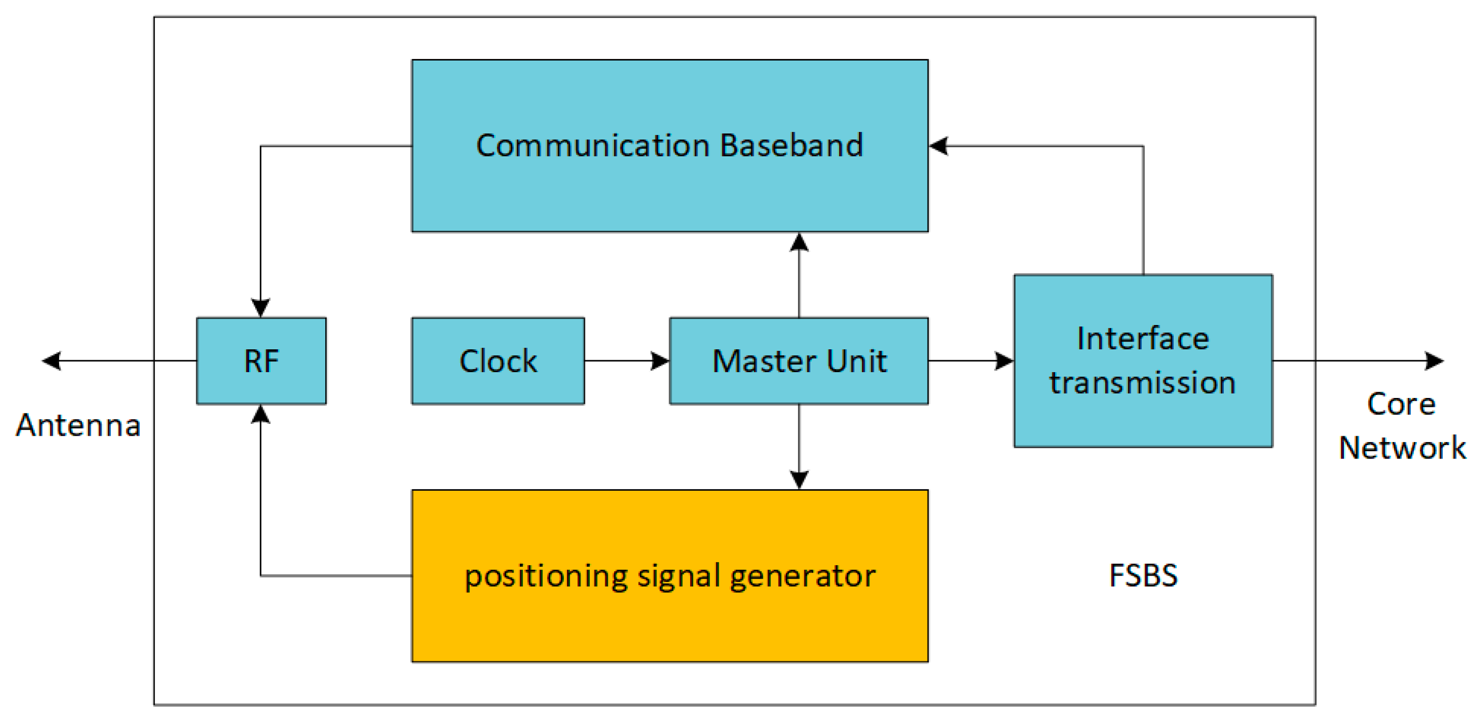
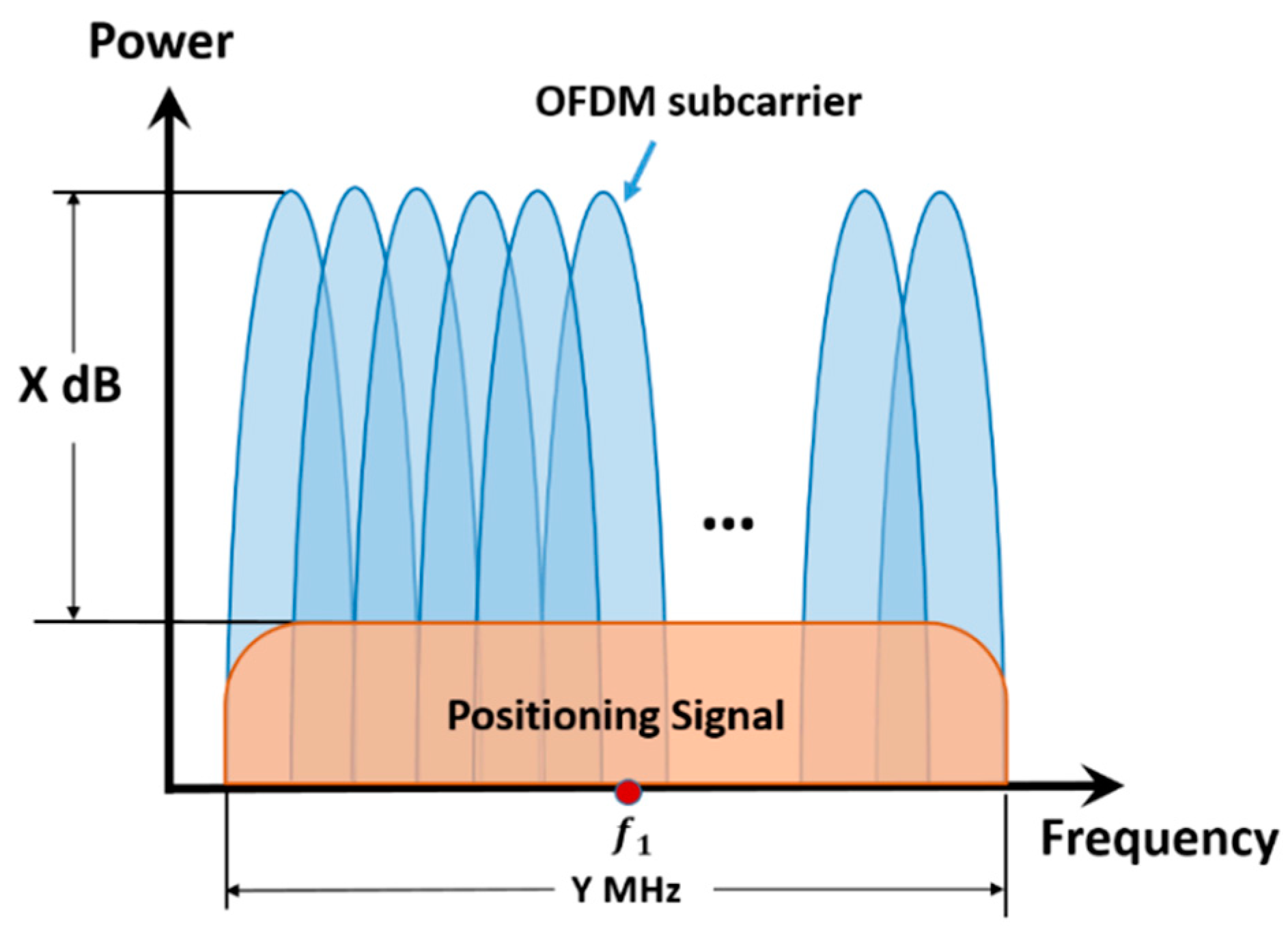
The navigation part in CNFS is a DSSS-CDMA system employing BPSK modulation as described above. FSBS can be built by integrating the positioning signal generator in the communication base station as shown in Figure 1. For the communication signal, the positioning signal can be regarded as noise. Radio-frequency (RF) module controls positioning signal power so that its power is low enough to not interfere with the communication signal. We can define the ratio of the positioning signal power to communication signal power as PCR. Based on a large number of experiments, the communication system can keep working properly when the PCR is lower than −18 dB. Figure 2 is a schematic diagram of the CNFS positioning signal and communication signal frequency spectrum. The communication signal in the 4G/5G communication system is based on original orthogonal frequency division multiplexing (OFDM) as shown in Figure 2.

Due to the difference of Frequency Division Duplexing (FDD) and Time Division Duplexing (TDD), the positioning signal needs to synchronize with the communication signal. If the downlink TDOA is only considered, CNFS positioning signal can be continuously transmitted in downlink frequency band when the communication system is FDD mode. However, TDD mode indicates the intermittent downlink communication signal. The synchronous downlink CNFS positioning signal is also intermittent. In this case, the fusion signal sent by the ith FSBS can be expressed as:

$$s^{\left(i\right)}\left(t\right)=s_{OFDM}^{\left(i\right)}\left(t\right)+s_P^{\left(i\right)}\left(t\right), t\in T_D$$

(1)

$$s_P^{\left(i\right)}\left(t\right)=d^{\left(i\right)}\left(t\right)c^{\left(i\right)}\left(t\right)cos\left(2\pi f_{c}t+\phi \right)$$

(2)

where $s^{\left(i\right)}\left(t\right)$ indicates the downlink fusion signal, $s_{OFDM}^{\left(i\right)}\left(t\right)$ indicates the downlink communication signal and $s_P^{\left(i\right)}\left(t\right)$ indicates the CNFS positioning signal. $T_D$ is the set of downlink duration. $d^{\left(i\right)}(t$) represents the navigation message, $c^{\left(i\right)}\left(t\right)$ denotes the PRN code, $f_c$ is the carrier frequency and $\phi$ is initial carrier phase. As mentioned above, the CI technique is utilized in CNFS positioning receiver to reduce the impact of the communication signal to the positioning signal. So the communication signal is ignored in the following analysis and the positioning signal is only considered.

2.2. FFT Acquisition Based on Partial Matched Filter

The positioning signals received by CNFS positioning receiver are converted to an intermediate frequency at first. And then, after converted by the analog-to-digital converter (ADC) module, the received signal can be expressed in the complex form as:

$$r\left(n\right)=Ad\left(n{T}_s\right)c\left(n{T}_s\right)e^{j\left(2\pi \left(f_{IF}+f_d\right)n{T}_s+{\phi }_0\right)}+v\left(n{T}_s\right).$$

(3)

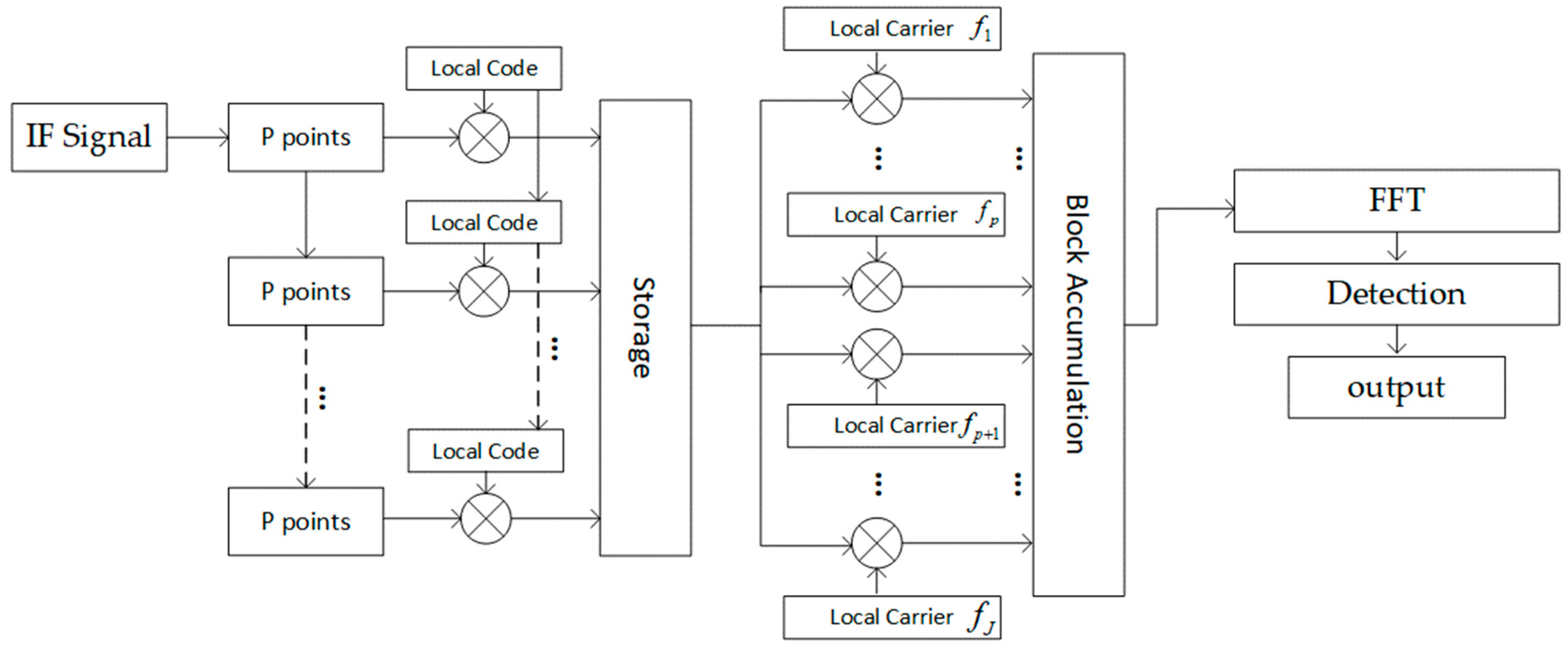
In Equation (3), we ignore the base station index i and focus on one base station. Where $T_s$ denotes the sampling duration, $A$ is the amplitude of the signal, $c\left(n{T}_s\right)$ is the PRN code utilized in CNFS, $d\left(n{T}_s\right)$ is the navigation message, $f_{IF}$ is the intermediate frequency, $f_d$ is the Doppler frequency, ${\phi }_0$ is the initial phase of the carrier and $v\left(n{T}_s\right)$ is the additive white Gaussian noise (AWGN) with one-sided power spectral density(PSD) of $N_0$.

The structure of the conventional PMF-FFT acquisition method is shown in Figure 3. P stands for the number of data processed in every match filter, which also represents the length of the match filter. It can be divided into two parts: partially matched filter and FFT module. Partially matched filter performs the PRN code phase search and FFT module performs the parallel frequency search in the frequency domain. The intermediate frequency of the positioning signal in CNFS is zero. The output of receiver RF front end $r\left(n{T}_s\right)$ is baseband signal with a Doppler frequency shift $f_d$. Then baseband signal is filtered by a group of matched filters with given local replica PRN codes being coefficients, whose output can be indicated as:

$$r_{PMF}\left(m\right)={\displaystyle \sum }_{n=Pm}^{P\left(m+1\right)-1}r\left(n\right)l\left(n\right), m=1,2,\dots ,N$$

(4)

where $P$ is the length of the match filter and $N$ is the number of match filter. Assuming the matched filter is implemented without navigation bit transition and the local code $l\left(n\right)$ is aligned with the PRN code of received signal, the response of each match filter with a noise-free signal can be written as:

$$r_{PMF}\left(m\right)=\left|\frac{sin\left(\pi f_{d}P{T}_s\right)}{sin\left(\pi f_d{T}_s\right)}\right|e^{j\left[\pi f_d{T}_s\left(P-1+2Pm\right)+{\phi }_0\right]}, m=1,2,\dots ,N.$$

(5)

The output of match filters is then passed to the FFT module. In practical application, the radix-2 FFT is mostly used for the convenience of operation, which can also be realized by FFT-ZP technique. Assuming that the length of FFT input data is $F\left(F\ge N\right)$. And the response of FFT can be expressed as:

$$\left|Y_{PMF-FFT}\left(k\right)\right|=\left|\frac{sin\left(\pi f_{d}P{T}_s\right)sin\left(\pi f_{d}NP{T}_s-\pi kN/F\right)}{sin\left(\pi f_d{T}_s\right)sin\left(\pi f_{d}P{T}_s-\pi k/F\right)}\right|, k=1,2,\dots ,F.$$

(6)

The derivation of Equations (5) and (6) can also be found in Reference [29,30,42]. We can finally acquire the PRN code phase and frequency estimation based on the FFT results. If the local code $l\left(n\right)$ is aligned with the PRN code of received signal, we can observe a peak in the amplitude response of FFT and the index of the peak indicates the frequency:

$$f_{est}=\{\begin{array}{c}{k}_p/PF{T}_s, k_p\le F/2\\ \left(k_p-F\right)/PF{T}_s, k_p>F/2\end{array}$$

(7)

where $f_{est}$ is frequency estimation result and $k_p$ is the peak index. The acquisition succeeds only when the peak is detected and the peak index is correct. There are several strategies to improve detection performance [38,39,43]. The signal SNR and amplitude response are the main factors that determine the detection result.

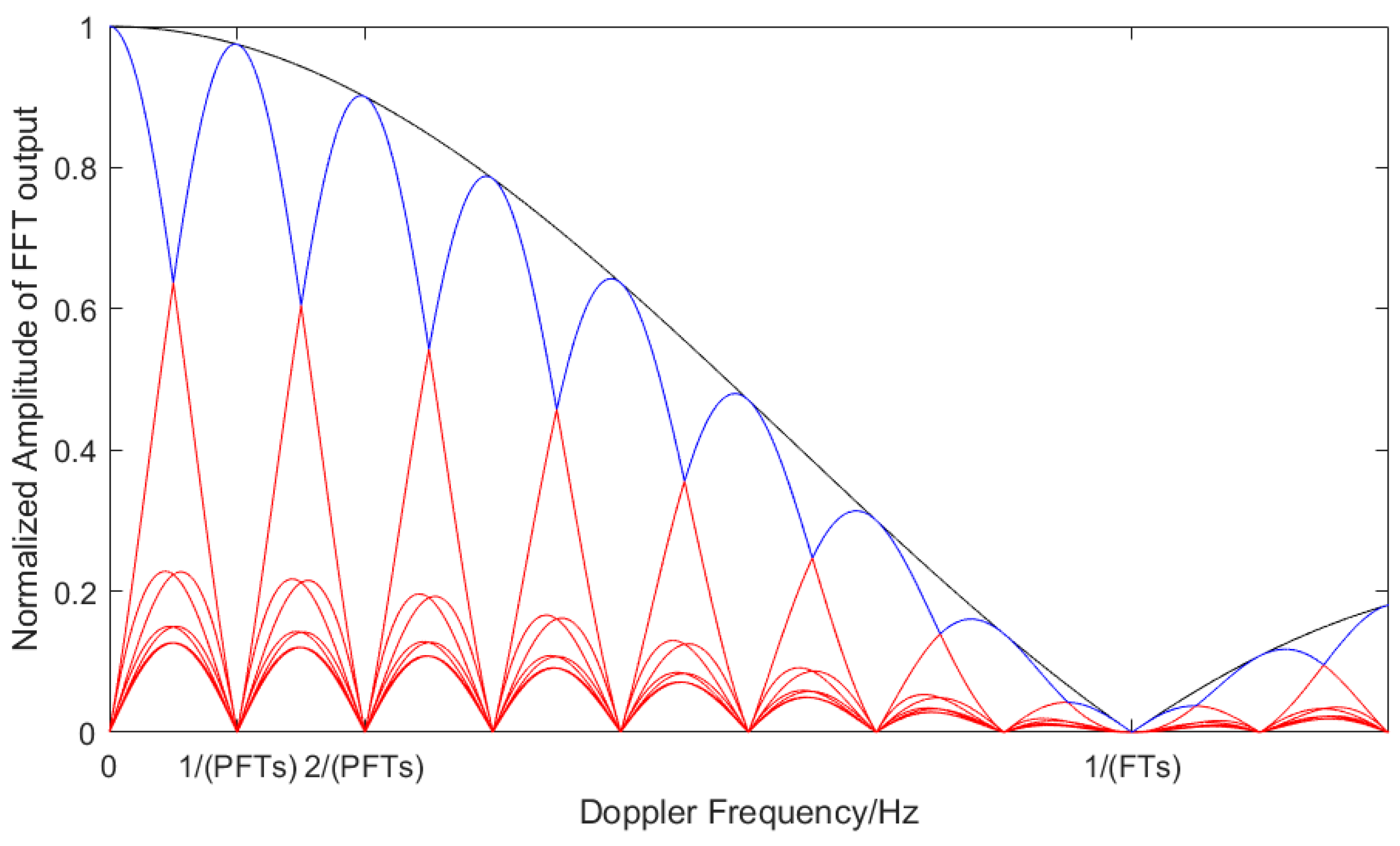
The amplitude response of the PMF-FFT output is mainly influenced by two factors based on Equation (5): the length of the match filter and the length of FFT. The total amplitude response envelope is affected by match filter length. Both the two factors decide the main lobe width of in each bin. These characters lead to the main drawback of PMF-FFT acquisition method mentioned in Section 1. The influence is shown clearly in Figure 4. The black line in Figure 4 indicates the amplitude response envelope and the blue line is the peak value of the amplitude response corresponding to a different frequency.

Besides the limited search range and the increase of computational load, we can observe two kinds of amplitude attenuation in Figure 4. One is coherent integration gain loss caused by frequency offset. The longer the integration time, the greater the amplitude attenuation. The other attenuation is caused by the picket fence effect. More exactly speaking, the FFT outputs will decline sharply when the frequency offsets of the received signal deviate from frequency intervals, especially when the frequency offset falls between two bins of FFT. These characters make it difficult to acquire accurate frequency estimation under weak signal environment.

3. Proposed Algorithm

3.1. PMF-FC-BA-FFT Acquisition Method

A new algorithm to realize the high-resolution frequency acquisition in a weak signal environment is proposed in this section. Frequency compensation (FC) was executed to avoid the amplitude attenuation and provide the ability to improve the frequency estimation accuracy. The block accumulation (BA) was performed to improve the SNR of the received signal. Based on the information obtained from FC, the interpolated FFT was implemented to acquire more accurate frequency estimation. The structure of the proposed method is depicted in Figure 5.

In order to explain the need for frequency compensation, we first analyzed the impact of block accumulation. Unlike conventional serial processing of sampling points, block accumulation is the overall operation of data blocks, which has been used in Reference [37,44]. The process of block accumulation is depicted in Figure 6.

If the local code $l\left(n\right)$ is aligned with the PRN code of the received signal, the PRN code in the output of PMF can be ignored. If we ignore the navigation message at the same time, the components in the received signal that should be considered are a carrier and the noise. Assuming that the signal to be processed is expressed as:

$$s\left(n\right)=e^{j\left(2\pi f^{\prime }n{T}^{\prime }+{\phi }_0\right)}+v^{\prime }\left(n\right)$$

(8)

where $f^{\prime }$ and $T^{\prime }$ are the frequency and sampling duration of signal respectively. $v^{\prime }\left(n\right)$ is the noise component. This operation divides the data into $L$ blocks and each block contains $M$ samples. Block accumulation can be described by the equation below:

$$s_{BA}\left(n\right)={\displaystyle \sum }_{i=0}^{L-1}s\left(n+iM\right)=A{e}^{j\left(2\pi f^{\prime }n{T}^{\prime }+{\phi }_0\right)}{H}_{BA}\left(f^{\prime }\right)+v_{BA}\left(n\right)$$

(9)

$H_{BA}\left(f_d\right)$ is the response of block accumulation and $v_{BA}\left(n\right)$ is the noise component after block accumulation. $H_{BA}\left(f_d\right)$ can be written as [37]:

$$H_{BA}\left(f^{\prime }\right)={{\displaystyle \sum }}_{i=0}^{L-1}{e}^{j2\pi f^{\prime }iM{T}^{\prime }}=\left|\frac{sin\left(\pi f^{\prime }M{T}^{\prime }L\right)}{sin\left(\pi f^{\prime }M{T}^{\prime }\right)}\right|e^{j2\pi f^{\prime }M{T}^{\prime }\left(L-1\right)}.$$

(10)

The block accumulation can be regarded as a filter, whose amplitude response is shown in Figure 7. It is clear that it has the character of frequency selectivity. The peaks of amplitude response appear at $h/\left(M{T}^{\prime }\right)$. $h$ is an integer. The zero-crossing bandwidth is $2/\left(ML{T}^{\prime }\right)$. We can draw the conclusion that the period of passband relies on the block size and the width of the main lobe depends on the block quantity. Only when the frequency of signal to be processed is within the range of $\left(h/\left(M{T}^{\prime }\right)-1/\left(ML{T}^{\prime }\right),h/\left(M{T}^{\prime }\right)+1/\left(ML{T}^{\prime }\right)\right)$, block accumulation can improve the SNR of signal.

The periodic character of the passband allows us to shift the signal frequency into the main lobe of the passband. That is the purpose of frequency compensation. By choosing a reasonable frequency compensation step, we can ensure that at least one signal is within the passband main lobe to avoid the attenuation caused by the frequency selectivity character of BA. The choice of frequency compensation step is associated with the block number $L$. The more the blocks, the smaller the frequency compensation step. The detailed explanation about the selection of frequency compensation step is described in detail in Section 3.2. The large attenuation due to the difference between the signal frequency and the center frequency of the main lobe can be reduced to an acceptable level. The matrix of frequency compensation is defined as:

$$\mathit{R}=\left[\begin{array}{ccc}1& e^{j2\pi \delta f{\mathit{n}}^{T}P{T}_s}& e^{j2\pi 2\delta f{\mathit{n}}^{T}P{T}_s}\end{array} \begin{array}{cc}\cdots & e^{j2\pi \left(J-1\right)\delta f{\mathit{n}}^{T}P{T}_s}\end{array}\right]$$

(11)

where $\delta f$ denotes frequency compensation step, $\mathit{n}$ is a row vector whose elements is from 1 to $N$, $\mathit{R}$ is a matrix whose size is $N\ast J$, $N$ is the data length after PMF. $J$ donates the number of frequency compensation components.

The parameters $M$, $T^{\prime }$ in Equation (10) were replaced with $N$, $P{T}_s$ respectively. The noise component was taken into account here. According to the structure in Figure 5 and Equations (5)–(10), the result after a partial match filter and frequency compensation can be expressed as the following equation:

$${\mathit{r}}_{\mathit{P}\mathit{M}\mathit{F}-\mathit{F}\mathit{C}}=r_{PMF}\left(\mathit{n}\right)\ast \mathit{R}\stackrel{\mathrm{def}}{=}{A}^{\prime }\mathit{G}+{\mathit{v}}_{\mathbf{1}}$$

(12)

$$A^{\prime }=A\left|\frac{sin\left(\pi f_{d}P{T}_s\right)}{sin\left(\pi f_d{T}_s\right)}\right|e^{j\left(\pi f_d\left(P-1\right)T_s+{\phi }_0\right)}$$

(13)

$$\mathit{G}\stackrel{\mathrm{def}}{=}\left[g_{n,j}\right],g_{n,k}=e^{j2\pi \left(f_d+j\delta f\right)nP{T}_s},n=1,2,\dots ,N,j=1,2,\dots ,J$$

(14)

where $g_{n,j}$ indicates the nth row and jth column element in matrix $\mathit{G}$. ${\mathit{v}}_{\mathbf{1}}$ is the noise component after PMF and FC. We obtained one block which had $N$ point samples every time we operate the PMF. After $L$ times operation, we can have $L$ blocks. Then the block accumulation was implemented. The $f^{\prime }$ in Equation (10) was replaced with $f_d+j\delta f$. The result of block accumulation can be expressed as:

$${\mathit{r}}_{\mathit{P}\mathit{M}\mathit{F}-\mathit{F}\mathit{C}-\mathit{B}\mathit{A}}=A^{\prime }{\displaystyle \sum }_{i=0}^{N-1}\left[g_{n+iL,j}\right]+{\mathit{v}}_2\stackrel{\mathrm{def}}{=}{A}^{\prime }\mathit{B}+{\mathit{v}}_2$$

(15)

$$\mathit{B}\stackrel{\mathrm{def}}{=}\left[b_{n,j}\right], b_{n,j}=\left|\frac{sin\left(\pi \left(f_d+j\delta f\right)NP{T}_{s}L\right)}{sin\left(\pi \left(f_d+j\delta f\right)NP{T}_s\right)}\right|e^{j2\pi \left(f_d+j\delta f\right)NP{T}_s\left(L-1\right)}{e}^{j\left(2\pi \left(f_d+j\delta f\right)nP{T}_s+{\phi }_0\right)}$$

(16)

where $v_2$ is the noise component after BA. FFT are then implemented. The output of FFT can be expressed as complex variable. The amplitude value of FFT output was used to execute the detection. And the amplitude response of FFT is expressed as:

$$\begin{gathered} {\mathit{Y}}_i\stackrel{\mathrm{def}}{=}\left[\left|y_{k,j}\right|\right] \\ \begin{array}{ll}\left|y_{k,j}\right|& =A\left|\frac{sin\left(\pi f_{d}P{T}_s\right)sin\left(\pi \left(f_d+j\delta f\right)NP{T}_s-\pi kN/F\right)sin\left(\pi \left(f_d+j\delta f\right)NP{T}_{s}L\right)}{sin\left(\pi f_d{T}_s\right)sin\left(\pi \left(f_d+j\delta f\right)P{T}_s-\pi k/F\right)sin\left(\pi \left(f_d+j\delta f\right)NP{T}_s\right)}\right|\\ & +V_{FFT}\end{array} \\ i=1,2,\dots ,I k=1,2,\dots ,F j=1,2,\dots ,J \end{gathered}$$

(17)

where the i indicates the matrix corresponding to ith code phase offset, I indicate the size of the code phase offset search space. $V_{FFT}$ is the noise component after FFT operation.

The detection strategy was then executed to decide whether the desired signal existed and to acquire the frequency and code phase offset estimation. Generally, the search space was a two-dimensional space of code phase and frequency offset. However, Equation (16) indicates that the search space of the proposed acquisition method was three-dimensional, one dimension for code phase search and two dimensions for frequency search. The whole search space is shown in Figure 8.

A novel MAX/TC detection criterion is proposed here to execute the detection. A common MAX/TC criterion divides the whole frequency and code phase uncertainty region into $I$ sectors with $F$ cells each. Inside a sector, a cell is selected according to the MAX criterion and the detection variables selected in each sector are compared to a threshold according to the TC criterion [38]. The detection criterion utilized in PMF-FC-BA-FFT method adds an extra maximum comparison between original MAX criterion and TC criterion. The cell-averaging constant false alarm rate (CA-CFAR) technique was utilized here to maintain a constant false alarm rate [45,46]. The detection process works as follows:

Step I: Compare every detection variable $\left|y_{k,j}\right|$ in column $j$ in matrix ${\mathit{Y}}_i$ and obtain the column max value $\left|y_{k_{max},j}\right|$.

Step II: After $J$ times FFT operation, compare $J$ column max value and obtain the matrix max value $\left|y_{k_{max},j_{max}}\right|$.

Step III: Calculate the threshold y_t based on CA-CFAR rules as equation below, where $\alpha$ is a threshold coefficient that can be adjusted based on different situations.

$$y_t=\frac{\alpha }{F-2}{\displaystyle \sum }_{k\notin \left(k_{max}-1, k_{max}+1\right)}\left|y_{k,j_{max}}\right|$$

(18)

Step IV: Compare $\left|y_{k_{max},j_{max}}\right|$ with $y_t$, if $\left|y_{k_{max},j_{max}}\right|\le y_t$, move to next matrix ${\mathit{Y}}_{i+1}$ and repeat steps from Step I to Step III, and if $\left|y_{k_{max},j_{max}}\right|>y_t$, make the decision that the desired signal presents.

Step V: Calculate the frequency and code phase offset estimation.

The code phase offset can be easily calculated according to the value of $i$. As for the frequency offset estimation, the two-step coarse-to-fine method is utilized here. The coarse frequency estimation is firstly acquired based on the equation below:

$$f_{ini}=\{\begin{array}{c}{k}_{max}/\left(FP{T}_s\right), k_{max}\le F/2\\ \left(k_{max}-F\right)/\left(FP{T}_s\right), k_{max}>F/2\end{array}$$

(19)

$$k_{max}=round\left(f_{j}FP{T}_s\right)$$

(20)

where $f_{ini}$ denotes the coarse frequency estimation, $round(·)$ denotes the nearest integer. The group number of signal whose frequency is closest to the center frequency of passband is obtained in previous step as $j_{max}$. Then the fine frequency estimation can be acquired based on the equation below:

$$f_{est}=\{\begin{array}{c}floor\left(f_{ini}NP{T}_s\right)/\left(NP{T}_s\right)-j_{max}\delta f, \left|y_{k_{max}+1,j_{max}}\right|<\left|y_{k_{max}-1,j_{max}}\right|\\ ceil\left(f_{ini}NP{T}_s\right)/\left(NP{T}_s\right)-j_{max}\delta f, \left|y_{k_{max}+1,j_{max}}\right|>\left|y_{k_{max}-1,j_{max}}\right|\end{array}$$

(21)

where $f_{est}$ denotes the final frequency acquisition result, $floor(·)$ denotes the nearest integer which is smaller than input, $ceil(·)$ denotes the nearest integer which is bigger than the input. The $floor(·)$ and $ceil(·)$ operation give the nearest passband center frequency.

3.2. Frequency Acquisition Accuracy

Equations (19) and (21) indicate that the accuracy of frequency estimation is influenced by many factors. The factors related to FC and BA process are analyzed here, which are frequency compensation step $\delta f$ and center frequency of passband. The $\delta f$ can be derived as follows:

$$\delta f=1/\left(JNP{T}_s\right).$$

(22)

A reasonable $\delta f$ can not only decrease the attenuation caused by the frequency selectivity character of BA but also increase the frequency acquisition accuracy. Equation (20) indicates that the $\delta f$ is directly decided by the number of frequency compensation components $J$. So the selection of $J$ is firstly analyzed.

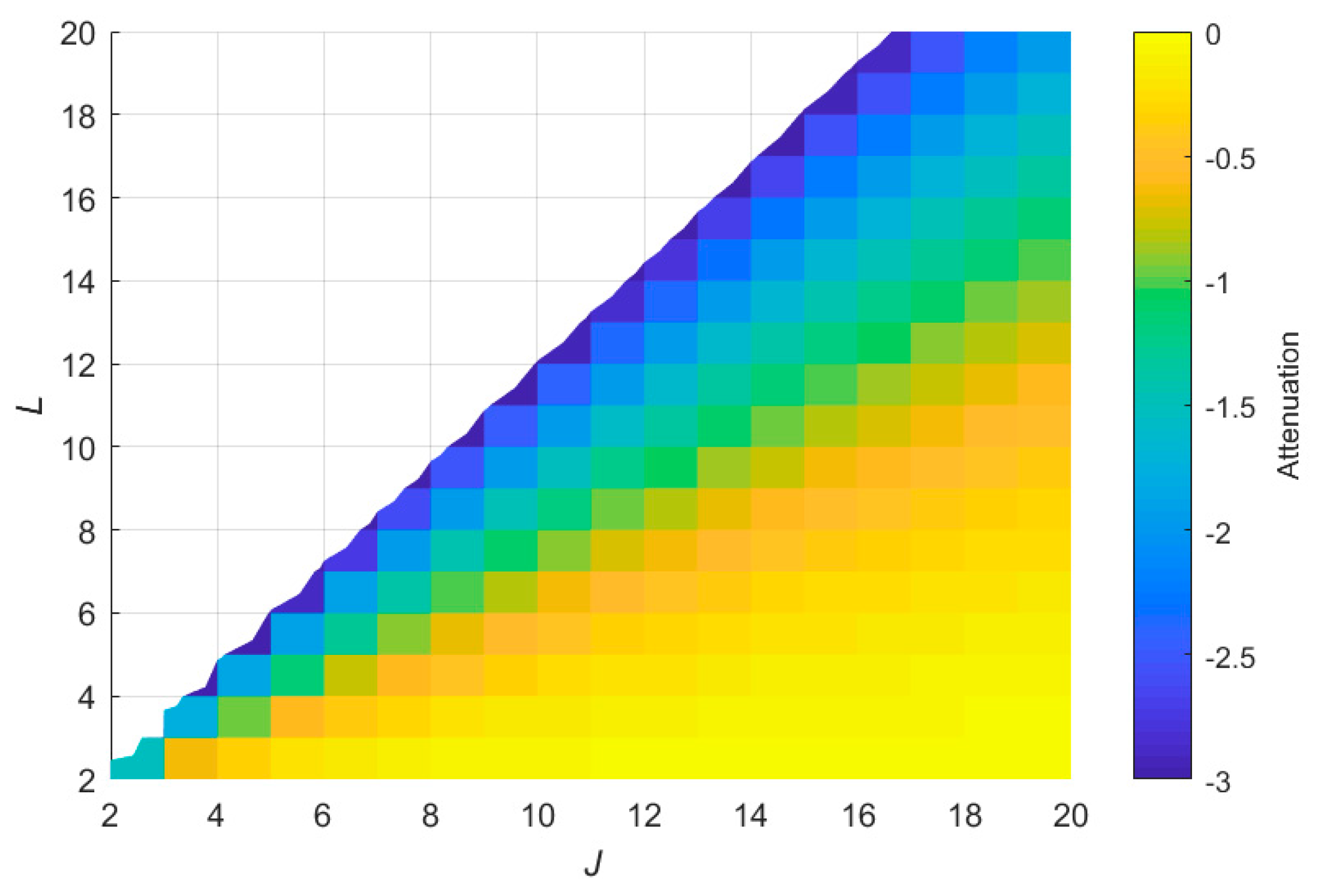
As the frequency $f_d$ of signal to be processed is unknown, the difference between frequency $f_d+j_{max}\delta f$ and the nearest center frequency $h_n/NP{T}_s$ is unknown. However, we can still analyze the attenuation directly caused by this difference. Considering the worst case, the center frequency $h_n/NP{T}_s$ is in the middle of $f_d+j_{max}\delta f$ and $f_d+\left(j_{max}+1\right)\delta f$ (or $f_d+\left(j_{max}-1\right)\delta f$). Then the difference is $\delta f/2=1/\left(2JNP{T}_s\right)$. The block number $L$ is also an important factor that influences the attenuation. Generally, 3dB is considered as the constraint of attenuation that can be accepted. Based on these considerations, the relation between max attenuation, the number of frequency compensation components $J$ and the block number $L$ can be shown as Figure 9 below:

The colored area in Figure 9 can meet the requirement of 3 dB. The relation between $J$ and $L$ also has an impact on computational load. Based on the structure of PMF-FC-BA-FFT method in Figure 5, no extra FFT module, which is the most computational resources consuming module, will be needed if $J\le L$. So the reasonable choice is $J=L$.

Under the condition of $J=L$, bigger $J$ leads to smaller attenuation and $\delta f$. Smaller $\delta f$ leads to an increased accuracy for frequency estimation. On the other hand, the requirement of acquisition time limits the selection of $J$. Thus, in the real environment, the value of $J$ from $J=2$ to $J=20$ can be considered based on different situation. The most common choice is $J=5$ and $J=10$.

The frequency acquisition accuracy of original PMF-FFT method can be derived from Equation (19). If we consider the worst case, the frequency acquisition error can be expressed as $1/\left(2FP{T}_s\right)$. And for PMF-FC-BA-FFT method, the frequency acquisition error can be derived easily based on the analysis above, which is $\delta f/2=1/\left(2JNP{T}_s\right)$. Considering the limitations of computational resources, $F$ is often chosen as $F\le 2N$. So $1/\left(2JNP{T}_s\right)<1/\left(2FP{T}_s\right).$ In this case, the proposed method can have higher frequency acquisition accuracy than original PMF-FFT method. More detailed accuracy comparisons and analysis need to consider the parameter settings of the methods for comparison and will be given in Section 4.

3.3. Effect of Proposed Algorithm on SNR

Assuming the received signal $r\left(n\right)$ is corrupted by a complex zero-mean Gaussian noise with the variance of ${\sigma }^2$. Then after PMF and FC, the variance of the noise component in Equation (12) becomes

$$Var\left(v_1\left(m\right)\right)\stackrel{\mathrm{def}}{=}Var\left({{\displaystyle \sum }}_{n=Pm}^{P\left(m+1\right)-1}v\left(n\right)\right)={{\displaystyle \sum }}_{n=Pm}^{P\left(m+1\right)-1}Var\left(v\left(n\right)\right)=P{\sigma }^2.$$

(23)

As a matter of fact, the block accumulation has the same effect as a match filter for noise because the noise component in every sample after PMF still has the character of being independent of each other. So we can draw the conclusion that the block accumulation increases the noise power by a factor of $L$, which can be expressed as the equation below:

$$Var\left(v_2\left(n\right)\right)\stackrel{\mathrm{def}}{=}Var\left({\displaystyle \sum }_{i=0}^{L-1}{v}_1\left(n+iM\right)\right)={\displaystyle \sum }_{i=0}^{L-1}Var\left(v_{PMF}\left(n+iM\right)\right)=LP{\sigma }^2.$$

(24)

Still, block accumulation does not break the independence of the noise component. Considering only noise, every frequency component in FFT result can be regarded as the linear combination of $N$ noise components which is independent of each other. The variation of $V_{FFT}\left(k\right)$ can be expressed as:

$${\sigma }_n^2=Var\left(V_{FFT}\left(k\right)\right)=E\left({\left|V_{FFT}\left(k\right)\right|}^2\right)=Var\left(v_2\left(n\right)\right){\displaystyle \sum }_{n=0}^{N-1}{\left|e^{-j2\pi \frac{n}{F}k}\right|}^2=NLP{\sigma }^2.$$

(25)

The effect of these operations to the signal power can be derived from Equation (16). Different frequency offset and frequency compensation lead to different attenuation of signal power. However, we can still obtain a general conclusion. When $f_j\stackrel{\mathrm{def}}{=}{f}_d+j_{max}\delta f$ is in the passband of BA amplitude response, the signal power in FFT output which has the maximum value can be expressed as:

$$\begin{array}{ll}{P}_s=a^2& ={\left(A\right)}^2{\left|\frac{sin\left(\pi f_{d}P{T}_s\right)sin\left(\pi f_{j}NP{T}_s-\pi k_{max}N/F\right)sin\left(\pi f_{j}NP{T}_{s}L\right)}{sin\left(\pi f_d{T}_s\right)sin\left(\pi f_{j}P{T}_s-\pi k_{max}/F\right)sin\left(\pi f_{j}NP{T}_s\right)}\right|}^2\\ & \stackrel{\mathrm{def}}{=}{\left(A{N}^{\prime }L\prime P\prime \right)}^2\end{array}$$

(26)

where $a$ is defined as the amplitude of a desired signal, $round(·)$ denotes the nearest integer. The Equations (25) and (26) indicates that these operations improve the noise power by a factor of $NLP$ and the desired signal power by a factor of ${\left(N^{\prime }L\prime P\prime \right)}^2$. The SNR of the received signal is improved by a factor of $L{\prime }^{2}P{\prime }^2{N}^{\prime 2}/\left(LPN\right)$. Compared with the original PMF-FFT acquisition method, the implementation of block accumulation improves the SNR by a factor of $L{\prime }^2/L$.

3.4. Probability of False Alarm and the Probability of Detection

The signal acquisition can be seen as a statistical process, and the detection variable $\left|y_{k,j}\right|$ can be modeled as a complex random variable both when the desired signal is present or not. The detection variable $\left|y_{k,j}\right|$ contains only noise (denoted as the null hypothesis $H_0$) or both the desired signal and noise (denoted as the alternative hypothesis $H_1$) [36]. Based on the analysis above, the noise component in FFT output $y_{k,j}$ is complex white Gaussian noise with its real and imaginary components being of zero mean and variance ${\sigma }_n^2$. According to the probability theory, the detection variable amplitude $\left|y_{k,j}\right|$ should be subject to Rayleigh distribution under the hypothesis $H_0$. $y_{k,j}$ is replaced with $y$ in the following equation for convenience. The Probability Density Function (PDF) of $y$ under $H_0$ is expressed as:

$$f_n\left(y\right)=\frac{y}{{\sigma }_n^2}{e}^{-\frac{y^2}{2{\sigma }_n^2}},y\in H_0.$$

(27)

Under hypothesis $H_1$, the real component $real\left(y\right)~N\left(acos\theta ,{\sigma }_n^2\right)$ and imaginary component $imag\left(y\right)~N\left(asin\theta ,{\sigma }_n^2\right).$ So the detection variable $\left|y\right|$ should be Rice distributed under $H_1$ and the PDF is expressed as:

$$f_s\left(y\right)=\frac{y}{{\sigma }_n^2}{e}^{-\frac{y^2+a^2}{2{\sigma }_n^2}}{I}_0\left(\frac{ya}{{\sigma }_n^2}\right),y\in H_1$$

(28)

where $I_0(·)$ is the modified Bessel function of the first kind of zero order. The detection process described above has an extra step of comparison using MAX criterion. This step chooses one column that has maximal detection value and this column becomes the sector that can be used to execute MAX/TC criterion. The noise component in every cell in the sector is independent of each other. False alarm happens when $\left|y\right|>y_t$ under $H_0$. So the probability of false alarm can be expressed as:

$$P_{fa}=1-{[{{\displaystyle \int }}_0^{y_t}{f}_n\left(y\right)dy]}^F=1-{\left[1-e^{-\frac{y_t{}^2}{2{\sigma }_n^2}}\right]}^F.$$

(29)

Correct detection happens when $\left|y\right|>y_t$ under $H_1$. The detection probability can be derived as follows:

$$P_d={{\displaystyle \int }}_{y_t}^{\infty }{f}_s\left(y\right)dy=Q\left(\frac{a}{{\sigma }_n},\frac{y_t}{{\sigma }_n}\right)$$

(30)

where $Q(·)$ is the Marcum Q-function. The probability of false alarm and detection are used in the next section to analyze the performance of the proposed method under a weak signal environment in detail.

4. Simulation and Test Result

4.1. Simulation Conditions

Simulations tests were carried out to verify the performance of the proposed acquisition method. The PRN code utilized in positioning part of CNFS was Weil code whose length was 10,230. The code rate was 4.092 MHz. Thus, the duration of one PRN code period was 2.5 ms. The code bin in the acquisition stage was 0.5 chip. A list of other parameters of the PMF-FC-BA-FFT method is presented in

Table 1. PMF-FC-BA-FFT acquisition parameters.

Parameters	Value
Length of Match Filter	186
Number of Match Filter	110
Length of FFT	128
Block Number	10
Frequency Compensation step (Hz)	40

.

Based on the description in Section 1, the most common approach to improve the frequency acquisition accuracy for FFT based method was to extend the length of FFT by FFT-ZP technique. The FFT-ZP technique was applied in PMF-FFT and the PMF-FFT-ZP method was obtained for comparison. The radix-2 FFT was used in the positioning receiver for the convenience of FPGA operation. The length of FFT was converted into an integer power of 2. The frequency acquisition accuracy of FFT and the computational load both increased as the length of zero-padding increased. The chosen of zero-padding length required a trade-off between frequency acquisition accuracy and consumption of computational resources. The parameters of PMF-FFT-ZP method are listed in

Table 2. PMF-FFT-ZP acquisition parameters.

Parameters	Value
Length of Match Filter	186
Number of Match Filter	110
Length of FFT	256,512

.

The CI technique can be utilized in many acquisition methods to improve the SNR of the received signal by accumulating the data serially. Thus, the CI-PMF-FFT method was obtained for comparison. The application of CI technique in PMF-FFT method also leads to the improvement of frequency acquisition accuracy and the reduction of the frequency search range. The consumption of computational resources also needs to be taken into account at the same time. The serial accumulation is divided into two parts, one was executed in the match filter, and the other was executed in the FFT module. In this case, we can avoid the serious reduction of the frequency search range. The parameters of CI-PMF-FFT method are listed in

Table 3. CI-PMF-FFT acquisition parameters.

Parameters	Value
Integration Time	5 ms, 10 ms
Length of Match Filter	186,372
Number of Match Filter	110
Length of FFT	256

.

4.2. Computational Load

The computational load was firstly compared. The length of the match filter and FFT module were the main differences between these three methods. Every partial match filter required $2P$ multipliers and $2P$ adders because the IQ demodulation utilized in the receiver. The computational resources of FFT module were $2F{\log }_{2}F$ multipliers, $3F{\log }_{2}F$ adders and $3F/2$ memory units. Besides, the frequency compensation and block accumulation required $2N$ multipliers, $2N$ adders and $10N$ memory units. If we saw the original PMF-FFT method which has 110 match filters whose length was 186 and 128 length FFT module as a basic reference. The extra computational resources required by these three methods are listed in

Table 4. Extra computational costs.

Resources	PMF-FC-BA-FFT	PMF-FFT-ZP (256)	PMF-FFT-ZP (512)	CI-PMF-FFT (5 ms)	CI-PMF-FFT (10 ms)
Multiplier	220	2304	7424	2304	2676
Adder	220	3456	11,136	3456	3828
Memory	1100	192	576	192	192

. We can see that the proposed method had a much lower cost on multipliers and adders compared with the other two methods. Even the memory cost was higher, the proposed method has advantages in computational cost.

4.3. Frequency Acquisition Accuracy

Secondly, we simulated the acquisition process of these three methods to obtain the frequency acquisition accuracy. All these three methods had different frequency estimation error when the frequency of the received signal was different. The carrier frequency of generated IF signal traversed all frequencies from 0 Hz to 1000 Hz in 1 Hz steps in the simulation and obtained the cumulative distribution function (CDF) of frequency estimation error. The simulations were conducted using MATLAB and every simulation is performed 100 times to obtain good statistical results.

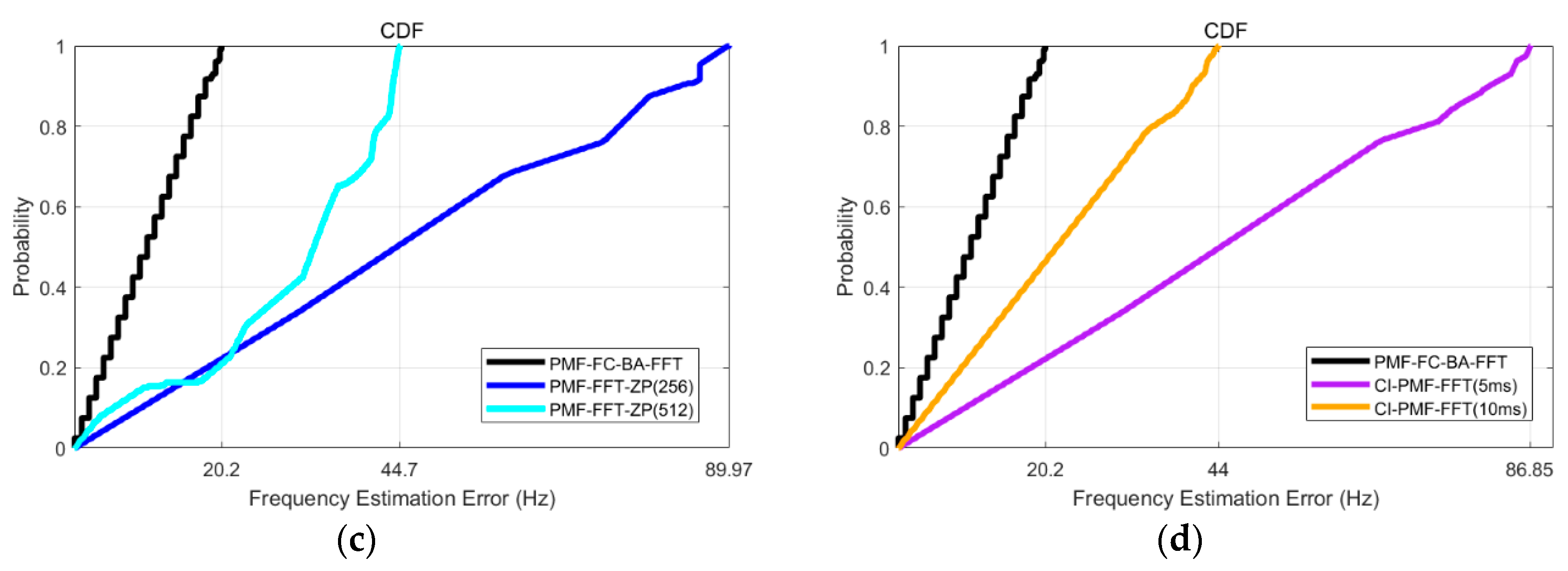
Coordinate values on the x-axis in Figure 10 indicate the maximum frequency acquisition error of these methods. We can first draw the conclusion that PMF-FC-BA-FFT method had the most accurate frequency acquisition result. On the other hand, the maximum error was theoretically half the search frequency bin and the CDF curve was theoretically a straight line without the existence of noise. We also compared the acquisition results when the SNR is different. The SNR in Figure 10a–d was −20 dB, −20 dB, −26 dB and −26 dB respectively. In order to make the comparison clearer, we divided the five methods for comparison into two parts under either SNR condition. Every method had better performance with higher SNR and the proposed method had better performance compared with other methods under lower SNR environments. When the frequency of FFT input fell near the middle point of FFT frequency search bin, the attenuation caused by the fence effect reached its maximum and the existence of noise led to the wrong choice of peak value and peak index. This wrong detection occurred more frequently as SNR decreased. The frequency estimation error was higher under weak signal environment.

4.4. Acquisition Sensitivity

$P_d$, $P_{fa}$ and ROC curves were used to evaluate the performance of acquisition under weak signal environments. Figure 11a,b is the ROC curve of these five methods under different SNR environments. Better performance means the high probability of detection and the low probability of false alarm. The area under the curve (AUC) can effectively and intuitively represent the performance of the acquisition method. It is clear that the AUC of the proposed method was higher than other methods so the PMF-FC-BA-FFT acquisition method performed better under a weak signal environment. Normal operation of the receiver generally requires the probability of false alarm less than 0.05. There were only two methods of the five can meet the requirements of the high probability of detection when the SNR of the received signal was −35 dB according to Figure 11a. When the SNR was up to −26 dB, all these five methods met the requirements.

The threshold coefficient $\mathsf{\alpha }$ determine both the $P_d$ and $P_{fa}$. We obtained the result of $P_d$ and $P_{fa}$ corresponding to different threshold coefficient in Figure 12. The probability of a false alarm had nothing to do with SNR and was determined by the length of the FFT module. The longer the FFT module length, the higher the threshold coefficient required. The acquisition threshold coefficient that meets the $P_{fa}$ requirement corresponding to 3 FFT lengths was 4, 4.1, 4.3 respectively. If we consider 0.9 as the requirement of $P_d$, only PMF-FC-BA-FFT method and CI-PMF-FFT method with 10 milliseconds integration can reach this limit when the SNR is −35 dB.

The $P_d$ of these methods corresponding to different SNR was also compared. The threshold in Figure 13a,b was 5 and 4 respectively. All the five methods could meet the requirement of $P_d$ when SNR was greater than −28 dB and the threshold coefficient was 4. The receiver with the PMF-FC-BA-FFT method could work fine when the SNR of the received signal was −39 dB. Under the condition of $P_d\ge 0.9$, the SNR requirement of the proposed method was at least 3dB lower than the other two methods, which means the at least 3 dB improvement of acquisition sensitivity.

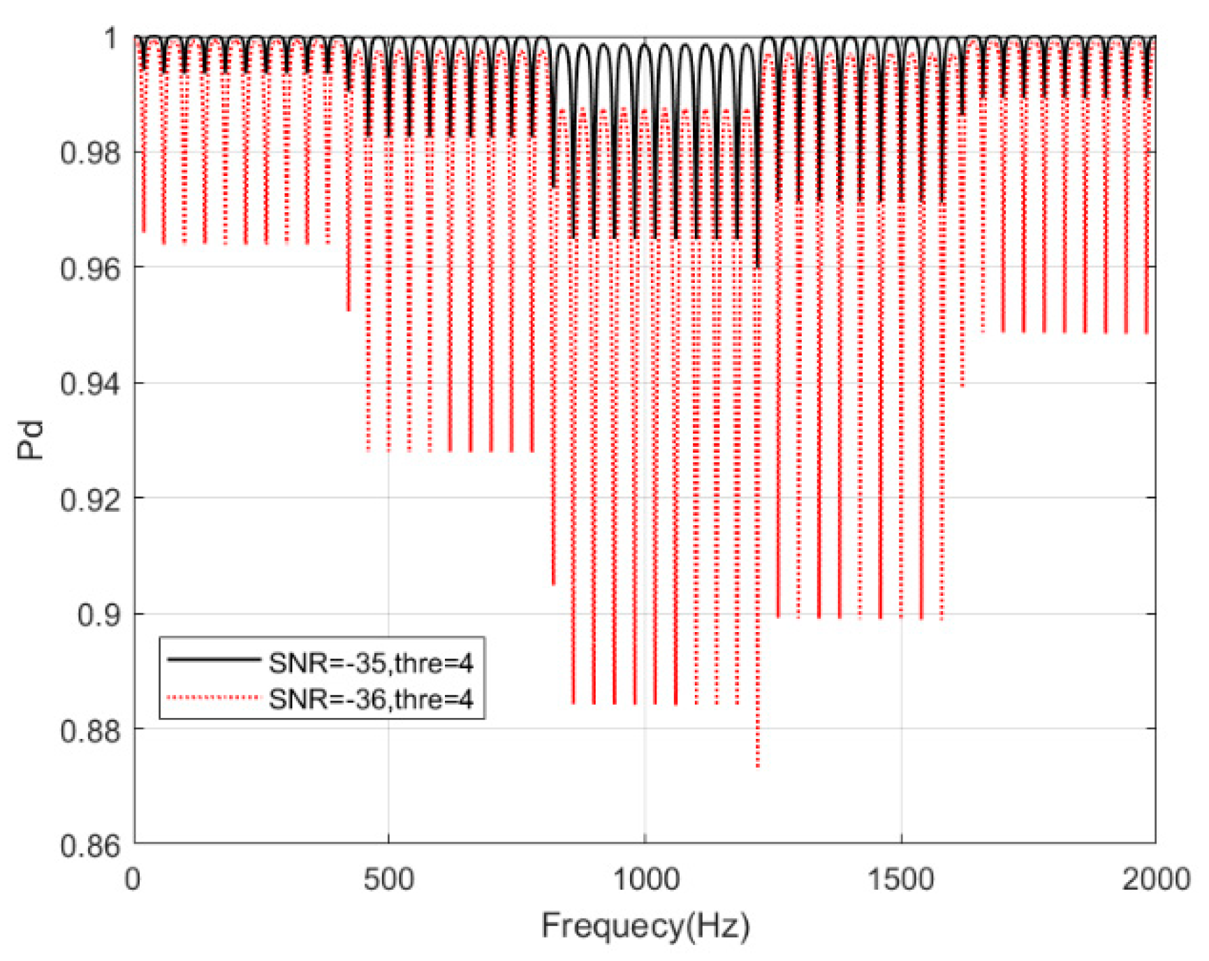
Meanwhile, signals with different frequency offset have different attenuation in PMF-FC-BA-FFT method so that the performance needs to be evaluated in terms of different frequency. All factors that cause attenuation were considered, which were match filter, block accumulation and FFT. The probability of detection corresponding to different frequency is shown in Figure 14. The threshold coefficient was set to 4 and met the requirement of the probability of a false alarm. When the attenuation caused by frequency offset was taken into account, the SNR that met the probability of detection requirement had risen to −36 dB. In other words, the frequency offset in PMF-FC-BA-FFT method caused 3 db attenuation. On the other hand, the attenuation that caused only by block accumulation was about 1.5 dB according to Figure 4.

The simulations above compare the computational load, frequency acquisition accuracy and the detection performance under different SNR of three methods with different parameters. It is clear that PMF-FC-BA-FFT acquisition method can obtain high accuracy frequency estimation result with fewer computational resources under weak signal environments.

4.5. Experimental Tests

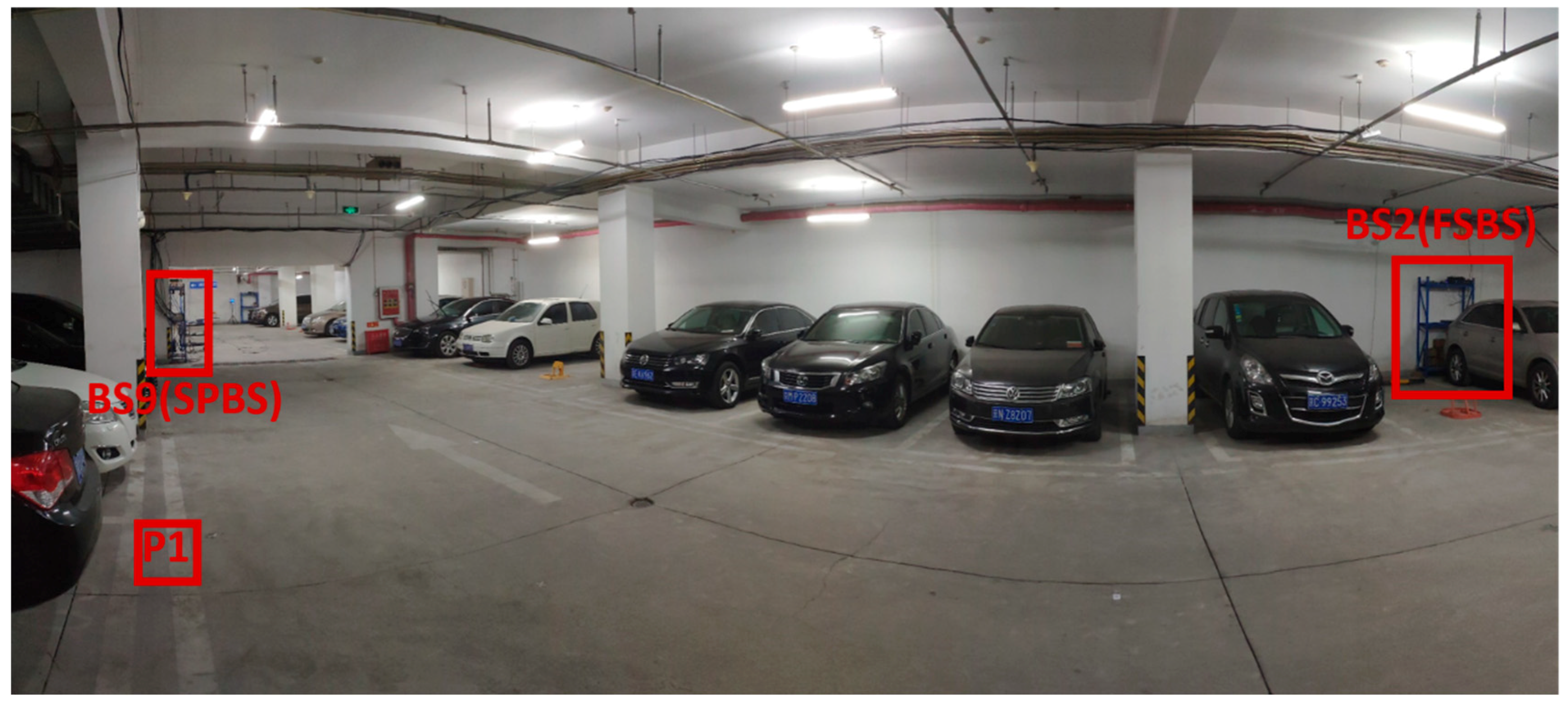
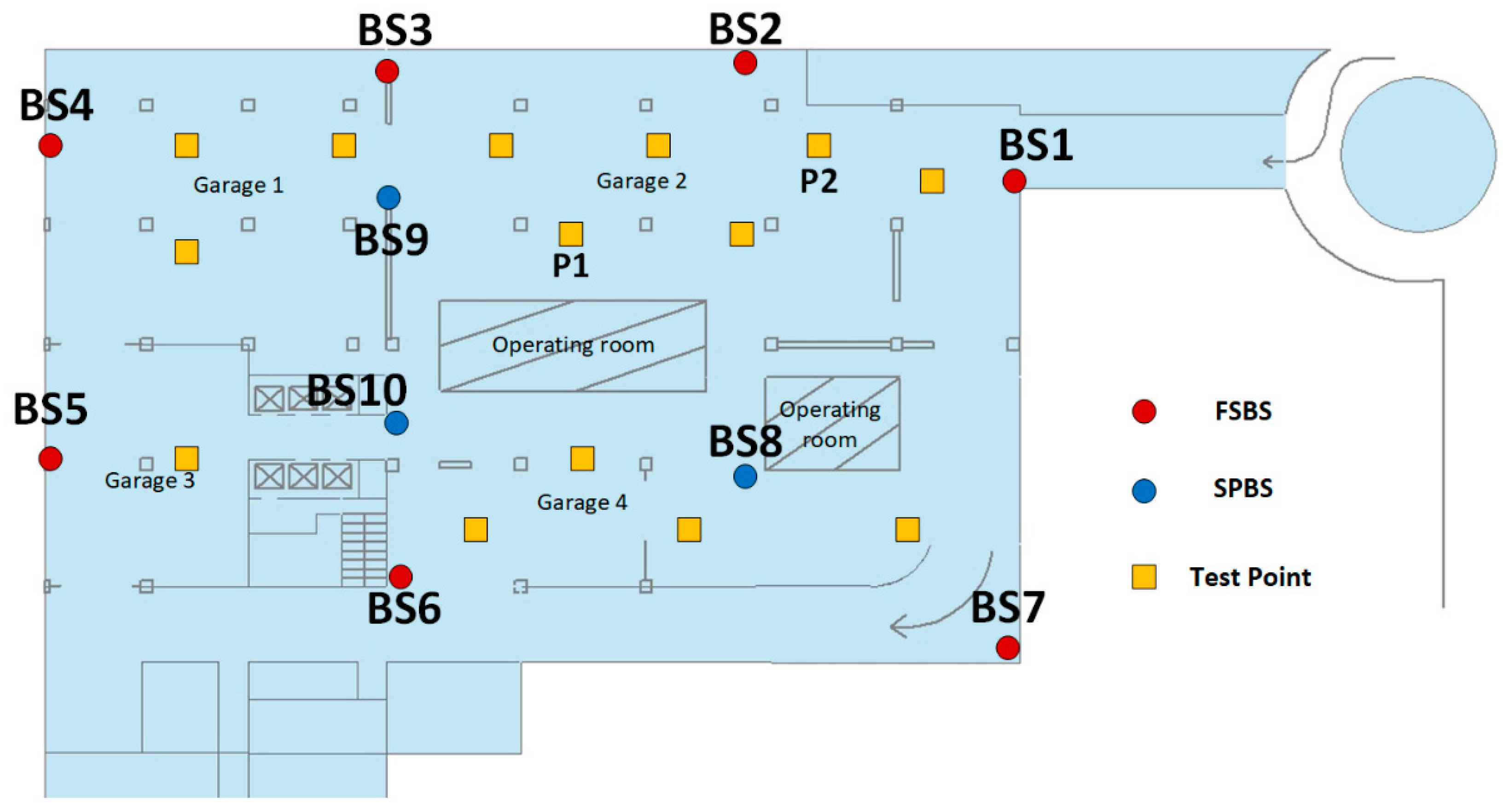
In order to assess the performance of the proposed method, experimental tests were conducted. The test field was an underground parking lot in Beijing University of Posts and telecommunications as shown in Figure 15. Base stations and test points are marked on the Figure. Specific information can be seen in Figure 16. Figure 16 is the plan of the whole test field, where the red circle points indicate the FSBS site and yellow rectangle points indicate the positioning test points. Several barriers like walls and rooms led to non-line-of-sight (NLOS) and multipath propagation. Though the NLOS and multipath detection approaches were utilized in the system, the severe attenuation of positioning signal was inevitable. Besides, the high sensitivity techniques, SPBS was also erected as the signal coverage supplements, which are indicated by the blue circle in Figure 16.

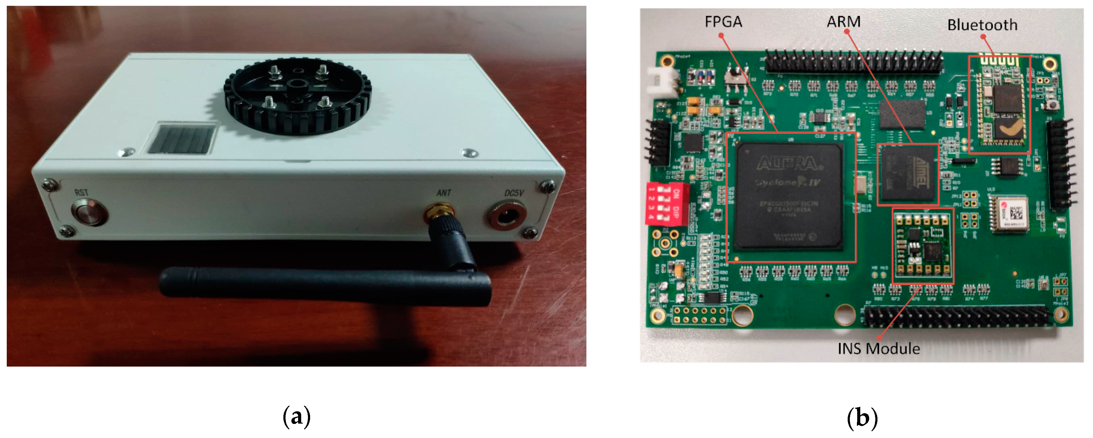
The equipment of the base station used in tests is shown in Figure 17. Figure 14 is the structure of positioning module. The atomic clock provided a reference clock signal and second pulse signal to the positioning module and the communication module. The positioning module generated the positioning signal mentioned above and the communication module generated 5 G NR communication signal. Both signals operated on the 3.5 GHz band. The communication module was a small cell for the indoor scenario. As mentioned above, we used a lower transmitting power of the positioning signal to avoid interference with the communication signal.

The positioning receiver used in tests is shown in Figure 18, which is an overview of internal and external structure. Positioning and other useful messages were transmitted from the positioning receiver to a mobile phone by Bluetooth. Finally, we used an app we developed on the mobile phone to display the positioning results. Baseband processing and data demodulation were conducted in FPGA and ARM processor on the positioning receiver board. The FPGA was chosen to have enough resources to implement the methods mentioned above. Besides, the INS module was also on board to realize multi-source fusion positioning when these functions are available. The acquisition was performed in FPGA and the methods were implemented in identical receivers to compare the acquisition results.

The acquisition results of PMF-FC-BA-FFT, PMF-FFT-ZP (512) and CI-PMF-FFT (10 ms) methods were firstly compared. In the experimental tests, plenty of test results of the receiver baseband process showed that the signals with low detection variables had worse stability due to the long and multipath propagation and the NLOS, which led to the unacceptable tracking results when the threshold coefficient corresponding to the signal detection variable was around 4, the corresponding signal could not be used in positioning calculation. On the other hand, the interference in the test environments such as the cross-correlation interference led to a higher false alarm rate than the simulation even with the cross-correlation cancelation technique. Therefore, a higher threshold can meet the requirements of the experimental tests. Based on this situation and plenty of test results, the threshold coefficient was set to 4.5 instead of 4, as mentioned above. Two typical test points P1 and P2 were chosen in Figure 16 and the acquisition results are shown in Figure 19. The number of base stations also indicates the PRN number. The signal of BS9 had the character of NLOS for test point P1 due to the existence of pillars, so the acquisition decision variable of BS9 was not the highest; even BS9 was the nearest base station for P1. It is clear that acquisition decision variables of existing signal in PMF-FC-BA-FFT method were higher than those in the other two methods, and weak signals can be acquired successfully using PMF-FC-BA-FFT.

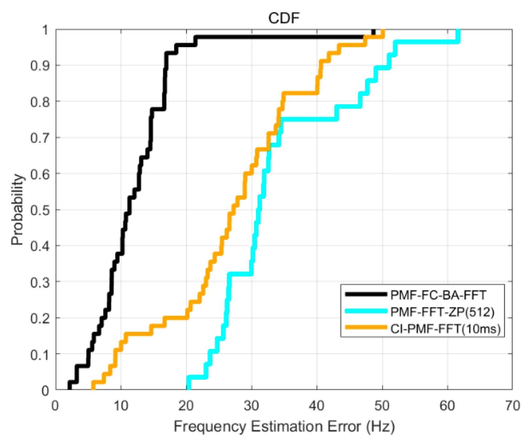
The difference between the receiver hardware, especially the crystal oscillator, will lead to the different residual carrier frequency of the same FSBS signal. In order to obtain the comparison results as accurate as possible, we compared the frequency acquisition results with the convergence result of the carrier tracking loop of every receiver individually. The crystal oscillator we used in the positioning receiver had good short-term stability, so the residual carrier frequency did not change greatly when we ran the static test at every test point. In order to extend the frequency test range, a movement test with different movement speeds and the adjustments in the receiver digital down converter (DDC) was implemented to realize the different residual carrier frequency. By running the movement test with a speed from 0 m/s to around 5 m/s and different movement directions, the frequency differences were up to about 100 Hz. The adjustments in receiver DDC led to different intermediate frequencies which included 300 Hz, 600 Hz, 900 Hz and 1500 Hz. Every intermediate frequency was combined with 10 tests with different movement speeds. The accurate residual carrier frequency is obtained by saving the baseband data and doing the analysis on the computer. Then, we could get the frequency acquisition error. The methods for comparison were PMF-FC-BA-FFT, PMF-FFT-ZP (512) and CI-PMF-FFT (10 ms), and all there three methods were tested using the same positioning receiver. The CDF curves of frequency acquisition error were then obtained based on the test results in Figure 20. It is clear that the PMF-FC-BA-FFT method had the highest frequency acquisition accuracy compared with the other two methods.

5. Conclusions

This paper proposed a new high sensitivity acquisition method with high accuracy frequency estimation that can be used in new communication and positioning fusion system. Frequency compensation was first performed to avoid the attenuation caused by the frequency selective filter characteristic of block accumulation and provide smaller frequency search step. Serial accumulation was replaced with block accumulation to avoid the decrease of the frequency search range in PMF-FFT method. Based on the analysis, simulation and experimental test results, the following conclusions can be drawn:

PMF-FC-BA-FFT method can achieve high accuracy frequency acquisition result and effectively improve the acquisition sensitivity. Both the advantages were realized without causing the decrease of frequency search range. Though PMF-FC-BA-FFT method required more memory resource compared with PMF-FFT-ZP and CI-PMF-FFT methods, the less consumption in multiplier and adder resource were huge advantages. The frequency acquisition accuracy and acquisition sensitivity were closely related to the parameter settings and computational resource consumptions, so the accurate improvement effect was based on different situation. However, we can still draw the general conclusion that PMF-FC-BA-FFT method can at least improve the frequency acquisition accuracy by two times and the acquisition sensitivity by 3 dB compared with PMF-FFT-ZP and CI-PMF-FFT methods.

References

- Shamaei, K.; Khalife, J.; Kassas, Z.M. Exploiting LTE Signals for Navigation: Theory to Implementation. IEEE Trans. Wirel. Commun. 2018, 17, 2173–2189. [Google Scholar] [CrossRef] [Green Version]
- Mautz, R. Overview of current indoor positioning systems. Geod. Kartogr. 2009, 35, 18–22. [Google Scholar] [CrossRef]
- Peral-Rosado, J.A.D.; Raulefs, R.; López-Salcedo, J.A.; Seco-Granados, G. Survey of Cellular Mobile Radio Localization Methods: From 1G to 5G. IEEE Commun. Surv. Tutor. 2018, 20, 1124–1148. [Google Scholar] [CrossRef]
- Commission, F.C. FCC Wireless 911 Requirements. Available online: https://transition.fcc.gov/pshs/services/911-services/enhanced911/archives/factsheet_requirements_012001.pdf (accessed on 20 May 2019).
- Laoudias, C.; Moreira, A.; Kim, S.; Lee, S.; Wirola, L.; Fischione, C. A Survey of Enabling Technologies for Network Localization, Tracking, and Navigation. IEEE Commun. Surv. Tutor. 2018, 20, 3607–3644. [Google Scholar] [CrossRef] [Green Version]
- Peral-Rosado, J.A.D.; López-Salcedo, J.A.; Kim, S.; Seco-Granados, G. Feasibility study of 5G-based localization for assisted driving. In Proceedings of the 2016 International Conference on Localization and GNSS (ICL-GNSS), Barcelona, Spain, 28–30 June 2016; pp. 1–6. [Google Scholar]
- Otsason, V.; Varshavsky, A.; LaMarca, A.; de Lara, E. Accurate GSM Indoor Localization. In Proceedings of the UbiComp 2005: Ubiquitous Computing, Berlin, Heidelberg, 11–14 September 2005; pp. 141–158. [Google Scholar]
- Zang, H.; Baccelli, F.; Bolot, J. Bayesian Inference for Localization in Cellular Networks. In Proceedings of the 2010 Proceedings IEEE INFOCOM, San Diego, CA, USA, 14–19 March 2010; pp. 1–9. [Google Scholar]
- Bravo, A.M.; Moreno, J.I.; Soto, I. Advanced positioning and location based services in 4G mobile-IP radio access networks. In Proceedings of the 2004 IEEE 15th International Symposium on Personal, Indoor and Mobile Radio Communications (IEEE Cat. No.04TH8754), Barcelona, Spain, 5–8 September 2004; Volume 1082, pp. 1085–1089. [Google Scholar]
- Ericsson. Mobile Positioning System. Available online: https://www.ericsson.com/en/portfolio/digital-services/automated-network-operations/analytics-and-assurance/mobile-positioning-system (accessed on 20 May 2019).
- Paek, J.; Kim, K.-H.; Singh, J.P.; Govindan, R. Energy-efficient positioning for smartphones using Cell-ID sequence matching. In Proceedings of the 9th international conference on Mobile systems, applications, and services, Bethesda, MD, USA, 28 June–1 July 2011; pp. 293–306. [Google Scholar]
- Ibrahim, M.; Youssef, M. CellSense: An Accurate Energy-Efficient GSM Positioning System. IEEE Trans. Veh. Technol. 2012, 61, 286–296. [Google Scholar] [CrossRef]
- Liu, Y.; Shi, X.F.; He, S.B.; Shi, Z.G. Prospective Positioning Architecture and Technologies in 5G Networks. IEEE Netw. 2017, 31, 115–121. [Google Scholar] [CrossRef]
- Chen, C.Y.; Wu, W.R. Three-Dimensional Positioning for LTE Systems. IEEE Trans. Veh. Technol. 2017, 66, 3220–3234. [Google Scholar] [CrossRef]
- Fischer, S. Observed Time Difference of Arrival (OTDOA) Positioning in 3GPP LTE; Qualcomm: San Diego, CA, USA, 2014. [Google Scholar]
- Deng, Z.L.; Mo, J.; Jia, B.Y.; Bian, X.M. An Acquisition Scheme Based on a Matched Filter for Novel Communication and Navigation Fusion Signals. Sensors 2017, 17, 18. [Google Scholar] [CrossRef]
- Mo, J.; Deng, Z.L.; Jia, B.Y.; Jiang, H.J.; Bian, X.M. A Novel FLL-Assisted PLL With Fuzzy Control for TC-OFDM Carrier Signal Tracking. IEEE Access 2018, 6, 52447–52459. [Google Scholar] [CrossRef]
- Liu, W.; Bian, X.M.; Deng, Z.L.; Mo, J.; Jia, B.Y. A Novel Carrier Loop Algorithm Based on Maximum Likelihood Estimation (MLE) and Kalman Filter (KF) for Weak TC-OFDM Signals. Sensors 2018, 18, 22. [Google Scholar] [CrossRef]
- Yu, S.C.; Deng, Z.L.; Jiao, J.C.; Jiang, S.; Mo, J.; Xu, F.H. The Multipath Fading Channel Simulation for Indoor Positioning. In China Satellite Navigation Conference; Sun, J., Liu, J., Fan, S., Wang, F., Eds.; Springer: New York, NY, USA, 2016; Volume 389, pp. 341–347. [Google Scholar]
- Deng, Z.; Yu, Y.; Yuan, X.; Wan, N.; Yang, L. Situation and development tendency of indoor positioning. Chin. Commun. 2013, 10, 42–55. [Google Scholar] [CrossRef]
- Boudreau, G.; Panicker, J.; Guo, N.; Chang, R.; Wang, N.; Vrzic, S. Interference coordination and cancellation for 4G networks. IEEE Commun. Mag. 2009, 47, 74–81. [Google Scholar] [CrossRef]
- Suman, P.; Baenke, J.; Harmon, A.; Irizarry, M.S.; Jakubek, R.; Leiterman, J.J.; Osman, A. Impact of Dirty Devices on CDMA Network Coverage and Capacity. IEEE Access 2015, 3, 752–758. [Google Scholar] [CrossRef]
- Cho, S.H.; Yeo, S.R.; Choi, H.H.; Park, C.; Lee, S.J. A design of synchronization method for TDOA-based positioning system. In Proceedings of the 2012 12th International Conference on Control, Automation and Systems, Jeju Island, Korea, 17–21 October 2012; pp. 1373–1375. [Google Scholar]
- Deng, Z.; Mo, J.; Jia, B.; Bian, X. A Fine Frequency Estimation Algorithm Based on Fast Orthogonal Search (FOS) for Base Station Positioning Receivers. Electronics 2018, 7, 376. [Google Scholar] [CrossRef]
- Wu, J.; Hu, Y. The Study on GPS Signal Acquisition Algorithm in Time Domain. In Proceedings of the 2008 4th International Conference on Wireless Communications, Networking and Mobile Computing, Dalian, China, 12–14 October 2008; pp. 1–3. [Google Scholar]
- Wen, H.; Meng, Z.; Teng, Z.S.; Guo, S.Y.; Yang, Y.X. Comparative Study of Influence of Noise on Power Frequency Estimation of Sine wave Using Interpolation FFT. Fluct. Noise Lett. 2014, 13, 11. [Google Scholar] [CrossRef]
- Wang, K.; Jiang, R.; Li, Y.; Zhang, N. A new algorithm for fine acquisition of GPS carrier frequency. GPS Solut. 2014, 18, 581–592. [Google Scholar] [CrossRef]
- Ren, T.; Petovello, M.G. A Stand-Alone Approach for High-Sensitivity GNSS Receivers in Signal-Challenged Environment. IEEE Trans. Aerosp. Electron. Syst. 2017, 53, 2438–2448. [Google Scholar] [CrossRef]
- Chang, L.; Jun, Z.; Zhu, Y.; Qingge, P. Analysis and optimization of PMF-FFT acquisition algorithm for high-dynamic GPS signal. In Proceedings of the 2011 IEEE 5th International Conference on Cybernetics and Intelligent Systems (CIS), Qingdao, China, 17–19 September 2011; pp. 185–189. [Google Scholar]
- Guo, W.F.; Niu, X.J.; Guo, C.; Cui, J.S. A new FFT acquisition scheme based on partial matched filter in GNSS receivers for harsh environments. Aerosp. Sci. Technol. 2017, 61, 66–72. [Google Scholar] [CrossRef]
- Zhang, H.L.; Ba, X.; Chen, J.; Zhou, H. FFT-based fine frequency estimation for weak GPS signal. J. Electron. Inf. Technol. 2015, 37, 2132–2137. [Google Scholar] [CrossRef]
- Tamazin, M.; Noureldin, A.; Korenberg, M.J.; Massoud, A. Navigation and Instrumentation Research Group. Robust fine acquisition algorithm for GPS receiver with limited resources. GPS Solut. 2016, 20, 77–88. [Google Scholar] [CrossRef]
- Borre, K.; Akos, D.M.; Bertelsen, N.; Rinder, P.; Jensen, S.H. A Software-Defined GPS and Galileo Receiver: A Single-Frequency Approach; Springer: Berlin, Germany, 2007. [Google Scholar]
- Tang, X.; Falletti, E.; Presti, L.L. Fine Doppler frequency estimation in GNSS signal acquisition process. In Proceedings of the 2012 6th ESA Workshop on Satellite Navigation Technologies (Navitec 2012) & European Workshop on GNSS Signals and Signal Processing, Noordwijk, The Netherlands, 5–7 December 2012; pp. 1–6. [Google Scholar]
- Pang, H.-S.; Lim, J.-S.; Kwon, O.-J.; Shin, B.J. Iterative Frequency Estimation for Accuracy Improvement of Three DFT Phase-Based Methods. IEICE Trans. Fundam. Electron. Commun. Comput. Sci. 2012, E95-A, 969–973. [Google Scholar] [CrossRef]
- Miller, M.; Nguyen, T.; Yang, C.; Blasch, E. Comparative study of coherent, non-coherent, and semi-coherent integration schemes for GNSS receivers. In Proceedings of the 63rd Annual Meeting of the Institute of Navigation 2007, Cambridge, MA, USA, 23–25 April 2007; pp. 572–588. [Google Scholar]
- Gao, F.Q.; Xia, H.X. Fast GNSS signal acquisition with Doppler frequency estimation algorithm. GPS Solut. 2018, 22, 13. [Google Scholar] [CrossRef]
- Corazza, G.E. On the MAX/TC criterion for code acquisition and its application to DS-SSMA systems. IEEE Trans. Commun. 1996, 44, 1173–1182. [Google Scholar] [CrossRef]
- Lu, W.J.; Zhang, Y.B.; Lei, D.Y.; Yu, D.S. Efficient Weak Signals Acquisition Strategy for GNSS Receivers. IEICE Trans. Commun. 2016, 99, 288–295. [Google Scholar] [CrossRef]
- Kim, B.; Kong, S.H. Determination of Detection Parameters on TDCC Performance. IEEE Trans. Wirel. Commun. 2014, 13, 2422–2431. [Google Scholar] [CrossRef]
- Kong, S.H.; Kim, B. Two-Dimensional Compressed Correlator for Fast PN Code Acquisition. IEEE Trans. Wirel. Commun. 2013, 12, 5859–5867. [Google Scholar] [CrossRef]
- Spangenberg, S.M.; Scott, I.; McLaughlin, S.; Povey, G.J.R.; Cruickshank, D.G.M.; Grant, P.M. An FFT-based approach for fast acquisition in spread spectrum communication systems. Wirel. Pers. Commun. 2000, 13, 27–56. [Google Scholar] [CrossRef]
- Tahir, M.; Lo Presti, L.; Fantino, M. A Novel Acquisition Strategy for Weak GNSS Signals Based on MAP Criterion. IEEE Trans. Aerosp. Electron. Syst. 2014, 50, 1913–1928. [Google Scholar] [CrossRef]
- Svaton, J.; Vejrazka, F. Pre- and Post-Correlation Method for Acquisition of New GNSS Signals with Secondary Code. In Proceedings of the 2018 IEEE/ION Position, Location and Navigation Symposium, Monterey, CA, USA, 23–26 April 2018; IEEE: New York, NY, USA, 2018; pp. 1422–1427. [Google Scholar]
- Benachenhou, K.; Hamadouche, M.; Taleb-Ahmed, A. New formulation of GNSS acquisition with CFAR detection. Int. J. Satell. Commun. Netw. 2017, 35, 215–230. [Google Scholar] [CrossRef]
- Oh, H.S.; Han, D.S. An adaptive double-dwell PN code acquisition system in DS-CDMA communications. Signal Process. 2005, 85, 2327–2337. [Google Scholar] [CrossRef]
Figure 1.
Structure of FSBS.
Figure 2.
Schematic diagram of the process of superposing positioning signal and communication signal.
Figure 3.
Structure of the PMF-FFT method.
Figure 4.
FFT output amplitude-frequency response.
Figure 5.
Structure of the PMF-FC-BA-FFT acquisition method.
Figure 6.
Block accumulation.
Figure 7.
Normalized amplitude response of block accumulation.
Figure 8.
Search space of the proposed algorithm.
Figure 9.
Relationship between max attenuation, the number of frequency compensation components J and block number L.
Figure 10.
(a) CDF of PMF-FC-BA-FFT and PMF-FFT-ZP when SNR was −20 dB; (b) CDF of PMF-FC-BA-FFT and CI-PMF-FFT when SNR was −20 dB; (c) CDF of PMF-FC-BA-FFT and PMF-FFT-ZP when SNR was −26 dB; (d) CDF of PMF-FC-BA-FFT and CI-PMF-FFT when SNR was −26 dB.
Figure 11.
(a) ROC curves when SNR was −35 dB; (b) ROC curves when SNR was −26 dB.
Figure 12.
(a) Probability of a false alarm corresponding to different threshold coefficient; (b) Probability of detection corresponding to different threshold coefficient when SNR was −35.
Figure 13.
(a) Probability of false alarm corresponding to different SNR when the threshold coefficient was 5; (b) Probability of detection corresponding to different SNR when the threshold coefficient was 4.
Figure 14.
Probability of detection corresponding to a different frequency.
Figure 15.
Realistic picture of the test field.
Figure 16.
Plan of the test field.
Figure 17.
(a) External structure of FSBS positioning module; (b) internal structure of FSBS positioning module; (c) FSBS.
Figure 18.
(a) External structure of CNFS positioning receiver; (b) internal structure of CNFS positioning receiver.
Figure 19.
Acquisition result of experimental tests using different acquisition method at test point P1 and P2. (a) PMF-FC-BA-FFT (P1); (b) PMF-FC-BA-FFT (P2); (c) PMF-FFT-ZP (512) (P1); (d) PMF-FFT-ZP (512) (P2); (e) CI-PMF-FFT (10 ms) (P1); (e) CI-PMF-FFT (10 ms) (P2).
Figure 20.
CDF curves of frequency estimation results.