Comparison of CNN Applications for RSSI-Based Fingerprint Indoor Localization


Division of Electronics and Electrical Engineering, Dongguk University-Seoul, Seoul 04620, Korea
*
Author to whom correspondence should be addressed.
Electronics 2019, 8(9), 989; https://doi.org/10.3390/electronics8090989
Submission received: 16 July 2019
/
Revised: 27 August 2019
/
Accepted: 2 September 2019
/
Published: 4 September 2019
(This article belongs to the Special Issue Indoor Localization: Technologies and Challenges)
Abstract
:The intelligent use of deep learning (DL) techniques can assist in overcoming noise and uncertainty during fingerprinting-based localization. With the rise in the available computational power on mobile devices, it is now possible to employ DL techniques, such as convolutional neural networks (CNNs), for smartphones. In this paper, we introduce a CNN model based on received signal strength indicator (RSSI) fingerprint datasets and compare it with different CNN application models, such as AlexNet, ResNet, ZFNet, Inception v3, and MobileNet v2, for indoor localization. The experimental results show that the proposed CNN model can achieve a test accuracy of 94.45% and an average location error as low as 1.44 m. Therefore, our CNN model outperforms conventional CNN applications for RSSI-based indoor positioning.
1. Introduction
Despite decades of research, effective products for indoor localization products are still unavailable, while indoor localization-based service demand continues to increase swiftly in smart cities [1]. Recent years have witnessed much indoor localization research. Most of the research aims to provide a widely used indoor localization scheme and achieve satisfactory performance similar to that of GPS in outside environments. Of these approaches [2,3,4,5], fingerprinting-based methods are the most widely used due to their effectiveness and the infrastructure’s independence. Fingerprinting-based localization methods include magnetic fingerprinting and Wi-Fi, both of which are based on the assumption that each location has a unique signal feature [6]. The fingerprinting localization process is usually divided into two phases: offline training and online processing. In the offline phase, Wi-Fi-received signal strength indicators (RSSI) or magnetic field strengths (MFS) at different reference points (RPs) are collected to construct a radio map. In the online phase, the user samples the RSSI or MFS data at their current position and finds similar signal patterns in the database. The corresponding location with the most similar pattern is regarded as the positioning result.
The intelligent use of machine learning (ML) techniques can assist in overcoming noise and uncertainty during fingerprinting-based localization. While traditional ML techniques work well at approximating simpler input-output functions, computationally intensive deep learning (DL) models are able to deal with more complex input-output mappings and can deliver superior accuracy. Middleware-based offloading [7] and energy enhancement frameworks [8]. Zafari et al. [9] may be an avenue to explore for computation and energy-intensive indoor localization services on smartphones. Furthermore, with the rise in the available computational power on mobile devices, it is now possible to deploy DL techniques such as convolutional neural networks (CNNs) on smartphones. A CNN is a special type of deep neural network (DNN) for image matching and recognition. The most popular aspect of CNN is that it can automatically identify necessary input features that have the most significant impact on the accuracy of the final output. This process is known as feature learning. Prior to DL, feature learning was an expensive and time-intensive process that had to be performed manually. CNN has been highly successful in complex image classification problems and is finding new applications in many emerging domains (e.g., self-driving cars) [10]. In this paper, we propose a new and efficient framework that employs CNN-based Wi-Fi fingerprinting to achieve a superior level of indoor localization accuracy for a user with a smartphone. Our approach utilizes widely available Wi-Fi access points (APs) without necessitating any customized/expensive infrastructure deployments. The framework works on a user’s smartphone, within the device’s computational capabilities, and utilizes the radio interfaces for efficient fingerprinting-based localization. This paper’s main novel contributions can be summarized as follows.
We constructed a CNN model with optimum performance for RSSI-based fingerprint indoor localization with dataset Schemes 1 and 2 [11], which were subsequently used to enhance indoor localization robustness and accuracy. In our previous work [11], we developed augmentation techniques for a CNN-based indoor positioning system. The CNN model in the previous work consisted of a five-layer network with three convolutional layers and two fully connected (FC) layers. The first FC layer contained 3072 nodes, and the second FC layer contained 1024 nodes, amounting to 4096 nodes. However, in this work, there are four convolutional layers and two FC layers with 2176 nodes in the first FC layer and 1024 nodes in the second FC layer and therefore 3200 nodes in total. This makes the total number of parameters 233,418, while the total number of parameters in [11] was 2,266,698, which was ~10 times higher than that of the current work. Therefore, with our proposed CNN model, test accuracy has been improved from 90.46% to 94.45% for Scheme 1 and 91.32% to 94.11% for Scheme 2.
We compared this model to different CNN applications, specifically AlexNet, ResNet, ZFNet, Inception v3, and MobileNet v2, for RSSI-based fingerprint datasets. We performed comprehensive testing of our algorithms with these CNN applications to demonstrate the effectiveness of our proposed framework. The remainder of the paper is structured as follows. First, Section 2 describes the previous work in this area. The type of dataset and CNN application along with our proposed CNN model can be found in the Methodology in Section 3. This leads to the experiments and results in Section 4.
2. Related Works
There are two main types of Wi-Fi-based indoor positioning technologies: the received signal strength indicator (RSSI)-based ranging positioning algorithm [12,13,14] and the fingerprint-based positioning algorithm [15,16,17]. The RSSI-based ranging positioning algorithm usually adopts the received Wi-Fi signal to estimate the distance between the target (its location is unknown) and the access point (its location is known) using the wireless radio signal propagation model and then estimates the target position using trilateration or multilateration methods. For example, in [12], a wireless mesh network (WMN) used a group of swarm robots equipped with wireless transceivers. This method used the approximate relative positions of the robots estimated by their RSSIs to deploy the WMN. The performance of Bluetooth low-energy (BLE) RSSI-based technology was explored for an indoor positioning system in different transmission conditions [13]. Another BLE-based scheme is proposed in [14], where the higher precision needed an extra training phase for localization. Fingerprint-based positioning methods were explored in a machine learning-based method that was developed in [15], where the support vector machine (SVM) was used to determine the different postures of the user. Jang et al. [16] provided an explicit survey for the limitation of an offline fingerprint map and overcame it with simultaneous localization and mapping (SLAM) methods. Meanwhile, Guan et al. [17] introduced a heuristic method to detect anomalous fingerprints under the framework of probabilistic fingerprint-based indoor positioning. A combination of the RSS-based fingerprint system presented in [18], where temporal signal variation is considered to construct a robust method for positioning, with the 15-month data collection time introduced here is used to overcome signal variation affecting localization.
With the rapid development of deep learning technology, some researchers have attempted to use deep learning methods in Wi-Fi positioning. Li [19] proposed tracking a user in an indoor environment by integrating a back-propagation neural network optimized through particle swarm optimization (PSO). In [20], a feed-forward neural network was adopted to detect the building and floor. To enhance location estimation, the centroid method was used in [20], and Hsieh [21] attempted to construct a recurrent neural network for indoor positioning. Variants of neural networks have been used in Wi-Fi positioning (e.g., deep belief networks [22], DNNs [23], fuzzy neural networks [24], and artificial synaptic networks [25]).
Since the above describe target positioning as a classification problem that relies on a collected fingerprint dataset, some regression algorithms have been applied, such as Gaussian regression [26], support vector machines (SVMs) [27], or combinations of these methods [28]. Jang et al. [29] presented robust image classification of the change in input data caused by the indoor multipath, where they built a 2D virtual radio map from the original 1-D Wi-Fi RSSI signal values and then constructed a CNN using 2-D radio maps as inputs. Channel state information (CSI)-based methods, such as [30,31,32,33,34], have proposed several ideas to process the CSI from Wi-Fi-based orthogonal frequency division modulation (OFDM) signals using deep CNNs. They fed the CSI directly into a CNN to train the position [30,31], train using phase information [32], directly estimate the angle of arrival with a CNN using phase fingerprinting [33], and combine these ideas [34]. However, the difference between their approaches and ours lies in the nature of the underlying signals and the system setup. RSSI-based localization requires a network of APs (i.e., a Wi-Fi network).
The DNN-based classifier in handwriting, such as MNIST in [35], has shown poor performance for untrained fonts, even for identical letters. The major drawback of DNN-based methods is that they are very sensitive to a change in the input data. To avoid this problem, the CNN was proposed. Recent studies have shown that the CNN-based classifier gives a satisfactory performance for image classification. The main advantage of a CNN is that it is able to learn the overall topology of an image via a convolution operation using a filter [36].
Various CNN applications were used for indoor positioning applications in [37,38,39,40]. A visual indoor positioning system was proposed in [37], where Alexnet was used to design a CNN for pedestrian activity recognition, which can serve as landmarks for indoor localization. Here, one-dimensional sensor data from accelerometers, magnetometers, gyroscopes, and barometers were considered network inputs. This work needed specific sensor types and did not consider an RSSI-based non-visual dataset. Valada [38] embedded geometric information derived from visual odometry. However, all of these approaches are dependent on ResNet residual network-based methods to estimate the ground truth camera poses required during fine-tuning the networks, which increases the infrastructure of the total system setup. Hanni [39] applied a transfer learning approach for indoor scene recognition, where the performance was compared with GoogLeNet and AlexNet. In this approach, a 3D image-type dataset was used to capture the spatial interrelationship, while in our approach an RSSI-based dataset is used, which generates a 2D grayscale image and achieves significantly higher accuracy than the state-of-the-art architectures AlexNet and GoogleNet. Modal 3D object detection in indoor environments using MobileNet [40] was used for an object detection network; the main idea of this network is reducing the computational operation for processing 3D positions even if they are covered with occlusions or cluttered by other objects. However, operating with 3D models increases the computational power uncertainty due to the noisy and incomplete reconstructed 3D shape. Therefore, a cost-effective method is always desirable to obtain a high-accuracy model. As shown in the above works, CNN applications are employed for a visual 3D dataset to train and test CNN applications for an indoor positioning application, which increases the total infrastructure of the indoor positioning system. Therefore, the main idea behind using an RSSI-based image setup is that it is the most user-friendly and infrastructure-free method. The terms user friendly and infrastructure free mean that there is no need to install additional devices to implement an RSSI-based indoor positioning system. The surrounding APs are sufficient for detecting the user’s location in an indoor environment with a smart device. We used a Wi-Fi RSSI-based dataset with optimized parameters and reduced complexity, which made it easy to implement and detect the indoor position without additional infrastructure demands.
3. Methodology
In this section, we will first introduce the experimental environment including the software and hardware configuration. Afterward, the proposed CNN-based method will be introduced as follows: the entire architecture of our CNN-based model, the data-processing approach, our network structure, related theories, and vital training strategies. Finally, we introduce the CNN application models and the fingerprint data image processing after each layer.
3.1. Hardware and Software Setup
The detailed software and hardware configuration information is given in Table 1. All our experiments were conducted on a server with powerful computational capabilities. The server contained 16 GB of memory and was equipped with two GeForce GTX 1080Ti graphics cards to accelerate computing. We installed Windows 10 in conjunction with Python. Python has very efficient libraries for matrix multiplication, which is vital when working with DNNs. TensorFlow is a very efficient framework for implementing the CNN architecture. We also installed dependencies, such as the CUDA Toolkit and CuDNN, before using TensorFlow. The CUDA Toolkit provides a comprehensive development environment for NVIDIA GPU-accelerated computing. CuDNN can optimize CUDA to improve the performance.
3.2. Input Datasets
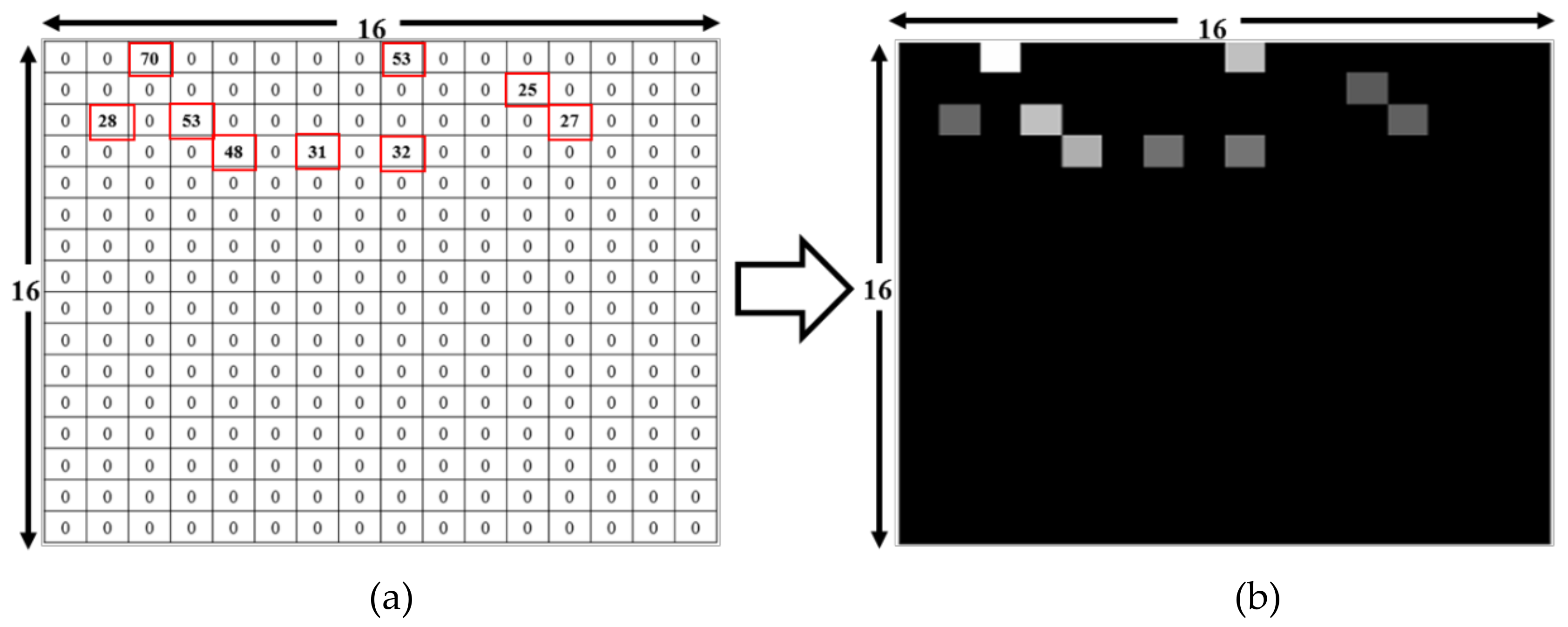
For our CNN model, a six-layer network was designed to predict 74 classes. The input image was generated from RSSI values received during the experiment with 74 RPs. At each RP, the RSSI value was recorded for 256 APs, though only a small subset of these APs was visible at each RP. These RSSI values from different APs created a 16 × 16 image. As shown in the example in Figure 1, there are nine visible APs out of 256 with RSSI values between 25 and 70, with the other APs having a value of 0. The RSSIs from different APs are converted into a grayscale image. The image brightness differs depending on the recorded RSSI values, with higher RSSI values being brighter. As shown in Figure 1a, the highest RSSI value is 70, which produces the brightest spot in the grayscale image shown in Figure 1b; the lowest value is 25, which is represented by the darkest nonblack spot. RSSI values of 0 produce no brightness, thus the remaining 247 spots are black. Similarly, the input RSSI files for the other 73 RPs produced different images for input into the DL network.
Data Augmentation
As introduced in our previous work [11], data augmentation is commonly used to reduce the effect of overfitting in deep learning. This is done by expanding an existing dataset using only available data, whereby the learning algorithm can extract task-essential features more effectively. Big datasets are required to train deep learning models; such datasets are usually gathered by manual data collection or from existing databases. However, only limited datasets are available in some cases, and data augmentation can be employed to expand such datasets. Two augmentation schemes, Schemes 1 and 2, were used as the input available dataset. Scheme 1 focuses on less-detailed data, facilitating simple augmentation with respect to the RSSIs. From a small input data size (3–7 kilobytes), sizes of ~30–50 megabytes are achieved using this technique. Scheme 2 uses mean values and uniform random numbers to add information into the dataset. From the same input file size, 3 to 7 kilobytes, Scheme 2 output augmented data size is approximately 300 to 700 megabytes. There were 122,760 and 585,722 input training images using Scheme 1 and 2, respectively. The total number of test images for the lab simulations was 1479. We used both schemes as the input dataset given their similar performance, with the only difference being the size of the augmented datasets.
3.3. Various CNN-Based Methods
3.3.1. Our CNN Model
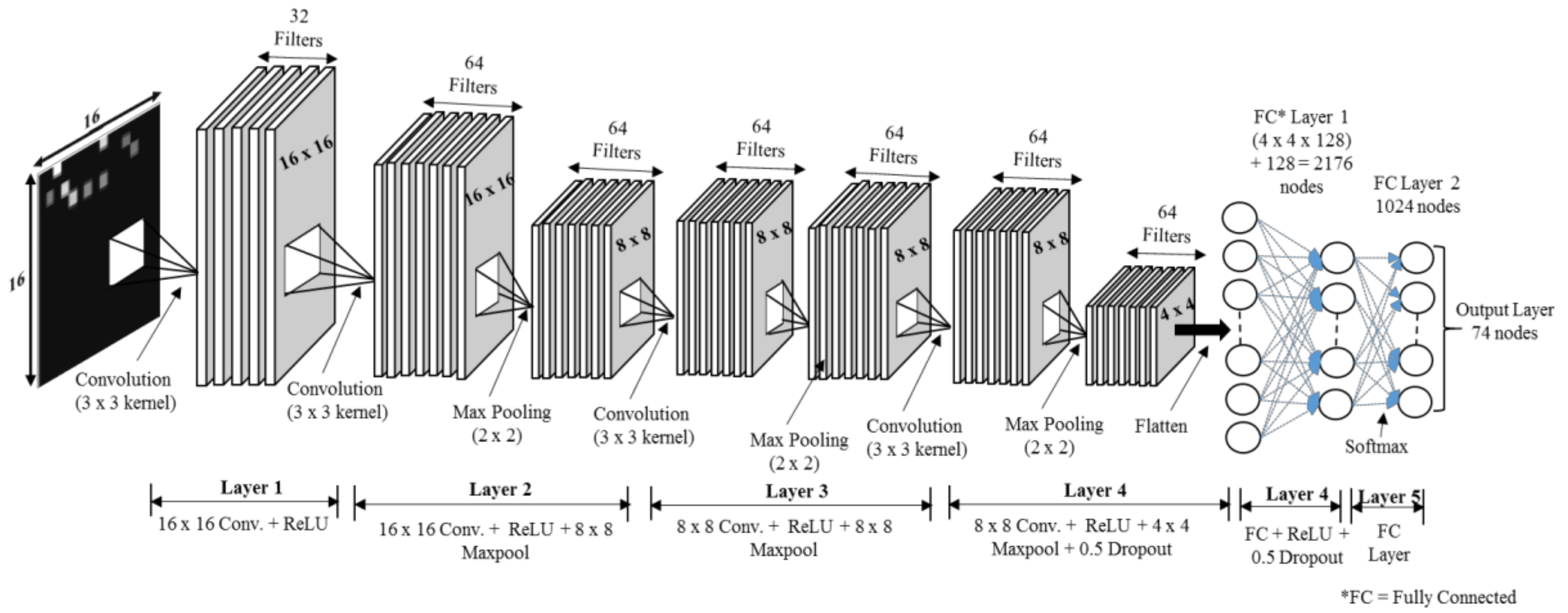
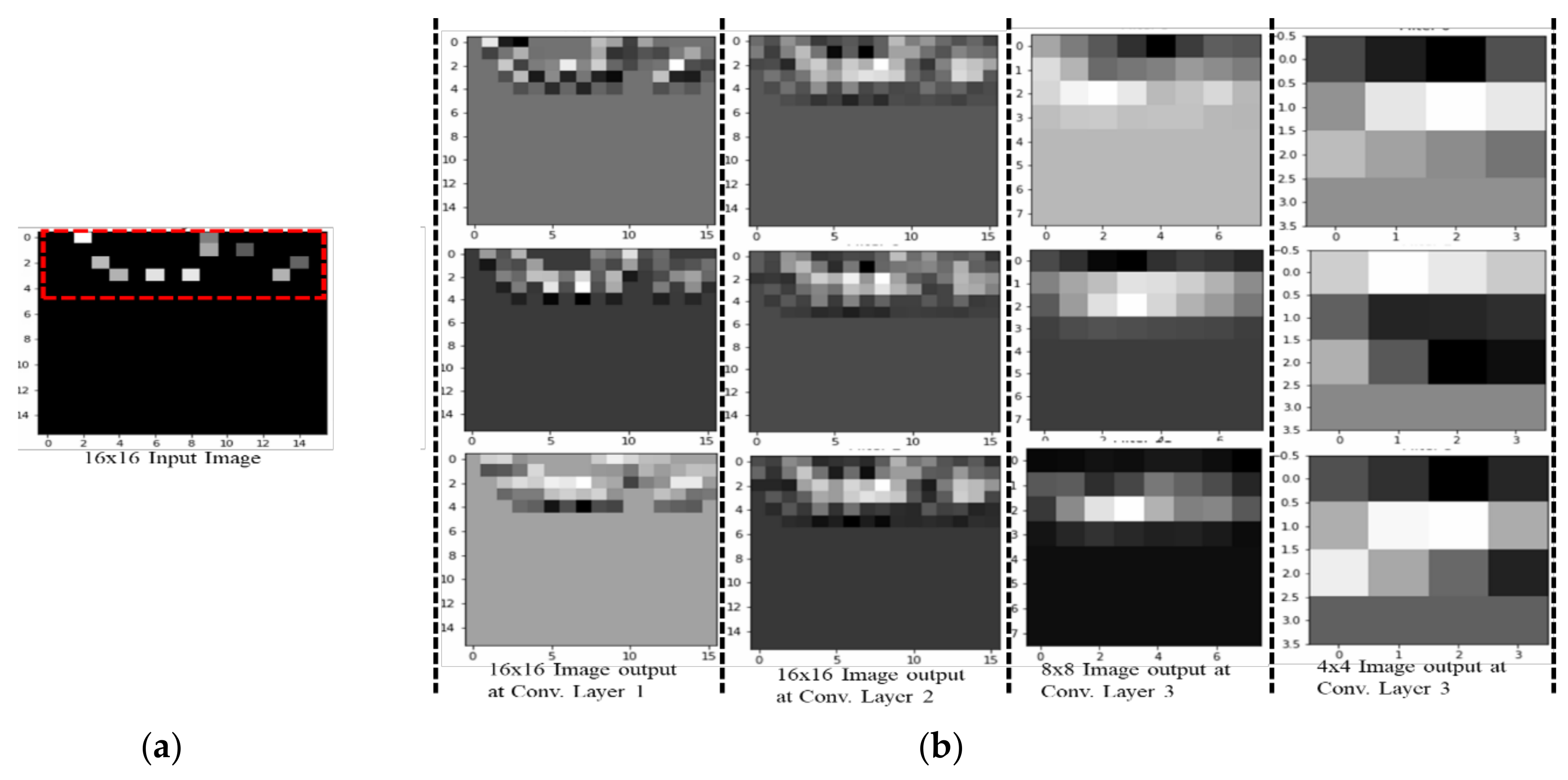
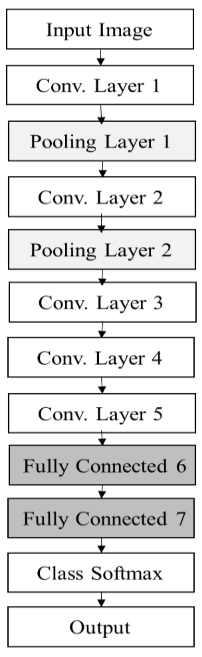
Figure 2 presents the architecture of our proposed method. Our CNN network comprises six layers, the first having input 16 × 16 × 1 grayscale images with rectified linear unit (ReLU) and dropout. Given the input dataset’s small size, the first layer does not use max pooling. The second layer consists of a 16 × 16 convolution with ReLU and an 8 × 8 max pooling layer with 18,496 parameters, and it produces output for the third 8 × 8 convolution layer (with ReLU and an 8 × 8 max pooling layer). This output is fed to the fourth layer, which is an 8 × 8 convolution layer with ReLU and an 8 × 8 max pooling layer. This output is fed directly to an FC layer with 2176 nodes, which leads to the next hidden FC layer, with 1088 nodes. Finally, the output is calculated using a softmax layer with 74 nodes, which is the total number of RPs in our setup. The inner width is 128, and the first three layers have no dropout, while the fourth layer uses a dropout of 0.5. The learning rate of our CNN model is 0.001, and the total number of parameters is 233,418. Table 2 summarizes all of the parameter settings. Figure 2 visualizes the activation of each convolutional network layer of our CNN model in a 2-dimensional (2D) grid. To generate the 2D image, the model is trained with RSSI dataset, and then the highest accuracy is used to visualize several kinds of features that a convolutional network learns at each layer of the network. Figure 3a represents an input image to pass through the network to visualize the network activation, and Figure 3b shows images of output that activates the neurons of the convolutional layers. The final image is generated at the softmax layer. It is important to note, here we are not using a deconvolutional layer; therefore, only features that a convolutional network learns at the following layers of the network is shown in the pictures.
3.3.2. AlexNet
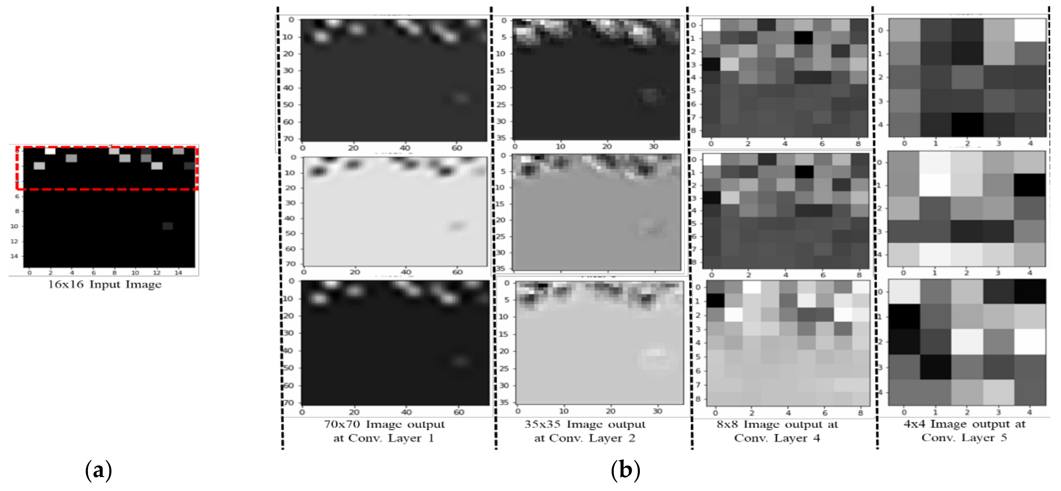
Benefitting from large datasets and parallel computing technology, AlexNet first achieved success on object classification tasks in 2012 [41], which substantially changed the field of DL in the computer vision community. As shown in Figure 4, AlexNet consists of five convolutional layers followed by two FC layers. The sizes of the convolution filters at the first and second convolutional layers are 11 × 11 and 5 × 5, respectively, but the size of the convolution filters at subsequent layers is 3 × 3. Figure 5 visualizes the activation of the 1st, 2nd, 4th, and 5th convolutional network layers for AlaxNet in a 2D grid.
3.3.3. ResNet
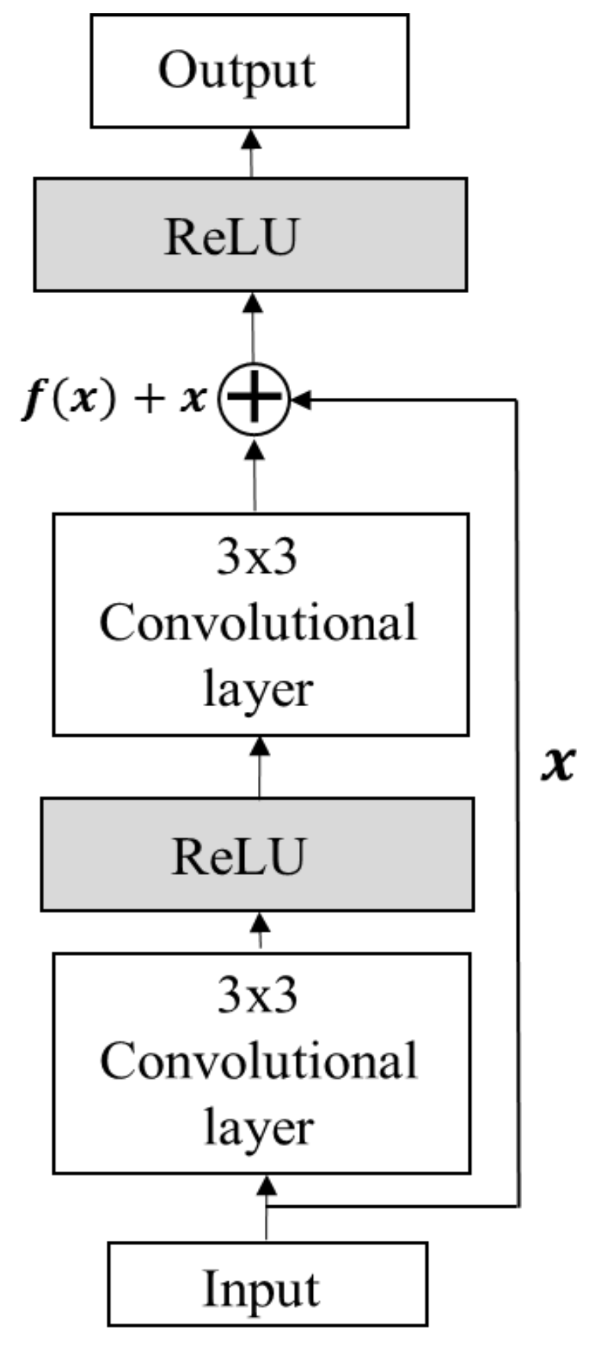
Residual neural networks (ResNets) were introduced in [42]. As shown in Figure 6, their basic building blocks are sequences of convolutions bypassed by skip connections, causing the model to learn residual values in the convolutional layers. The ResNet-50 model, introduced in [40], consists of 16 bottleneck blocks. The overall model contains 50 layers with trainable parameters, including a convolutional layer after the input layer and an FC output layer. Figure 7 visualizes the activation of the 1st, 2nd, 4th, and 5th convolutional network layers for ResNet in a 2D grid.
3.3.4. ZFNet
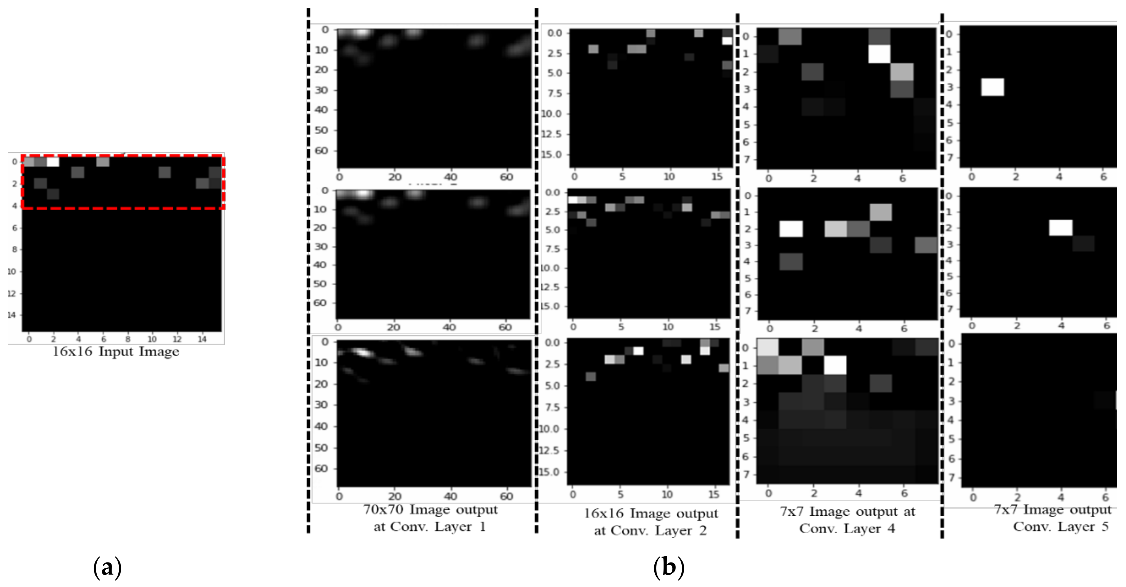
ZFNet was introduced in 2013, as [43] is a modified version of AlexNet with better accuracy. One major difference in the approaches is that ZFNet only uses 7 × 7 sized filters, compared to AlexNet’s 11 × 11 filters. The rationale is that larger filters entails loss of a lot of pixel information, which can be fixed by having smaller filter sizes in the earlier convolutional layers. As depth increases, the number of filters increases. ZFNet network also uses ReLUs for activation and was trained using batch stochastic gradient descent (Figure 8). Figure 9 visualizes the activation of the 1st, 2nd, 4th, and 5th convolutional network layers for ZFNet in a 2D grid.
3.3.5. Inception v3
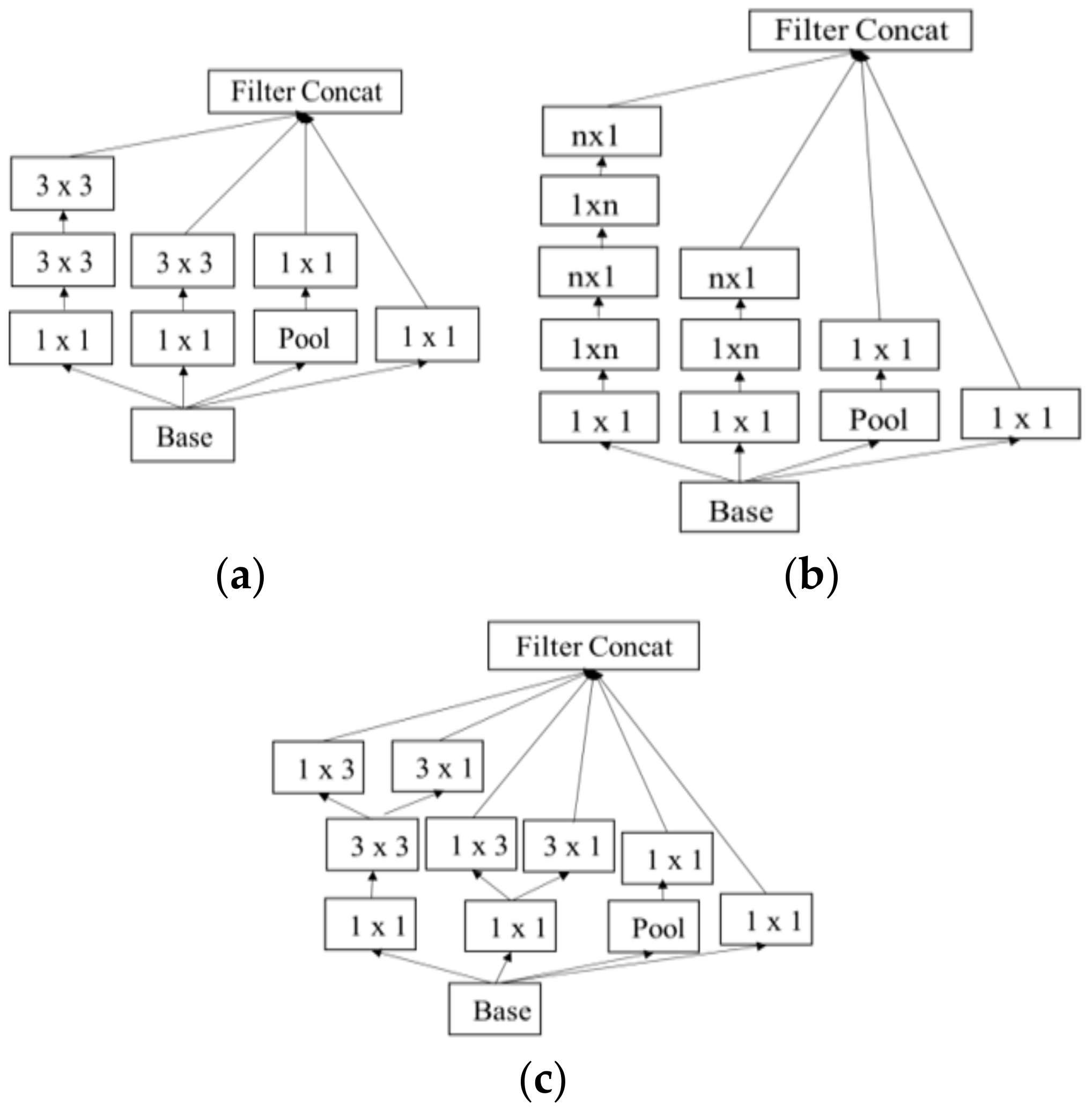
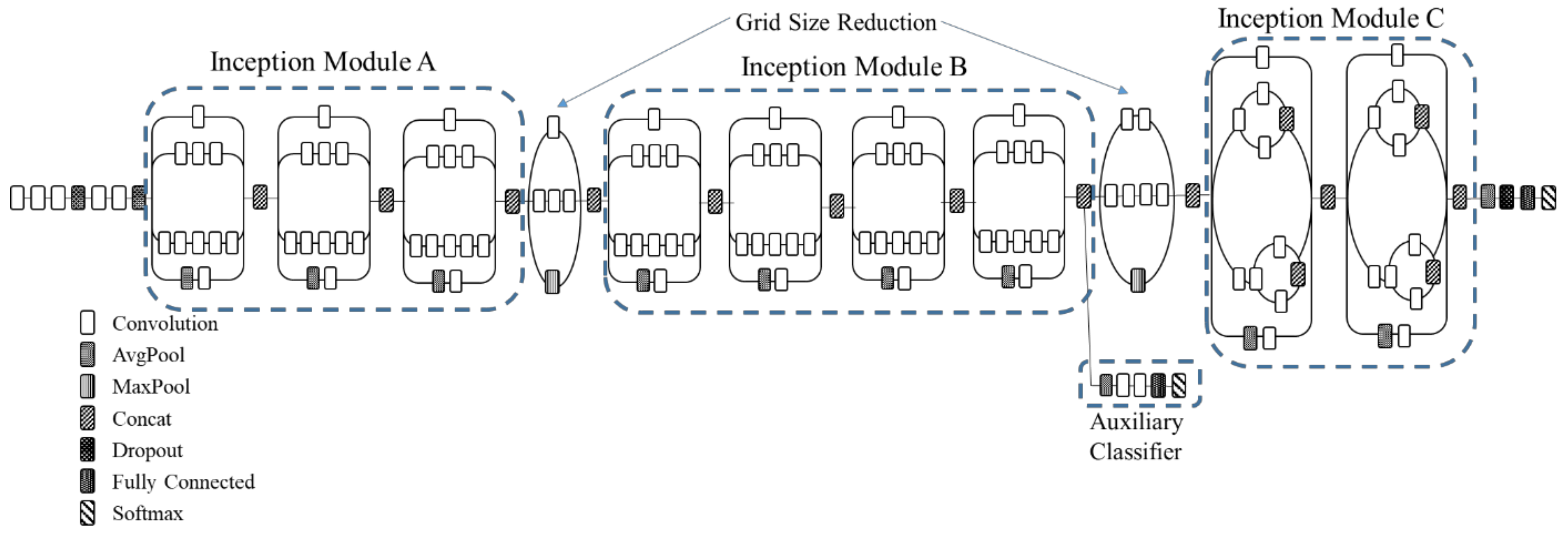
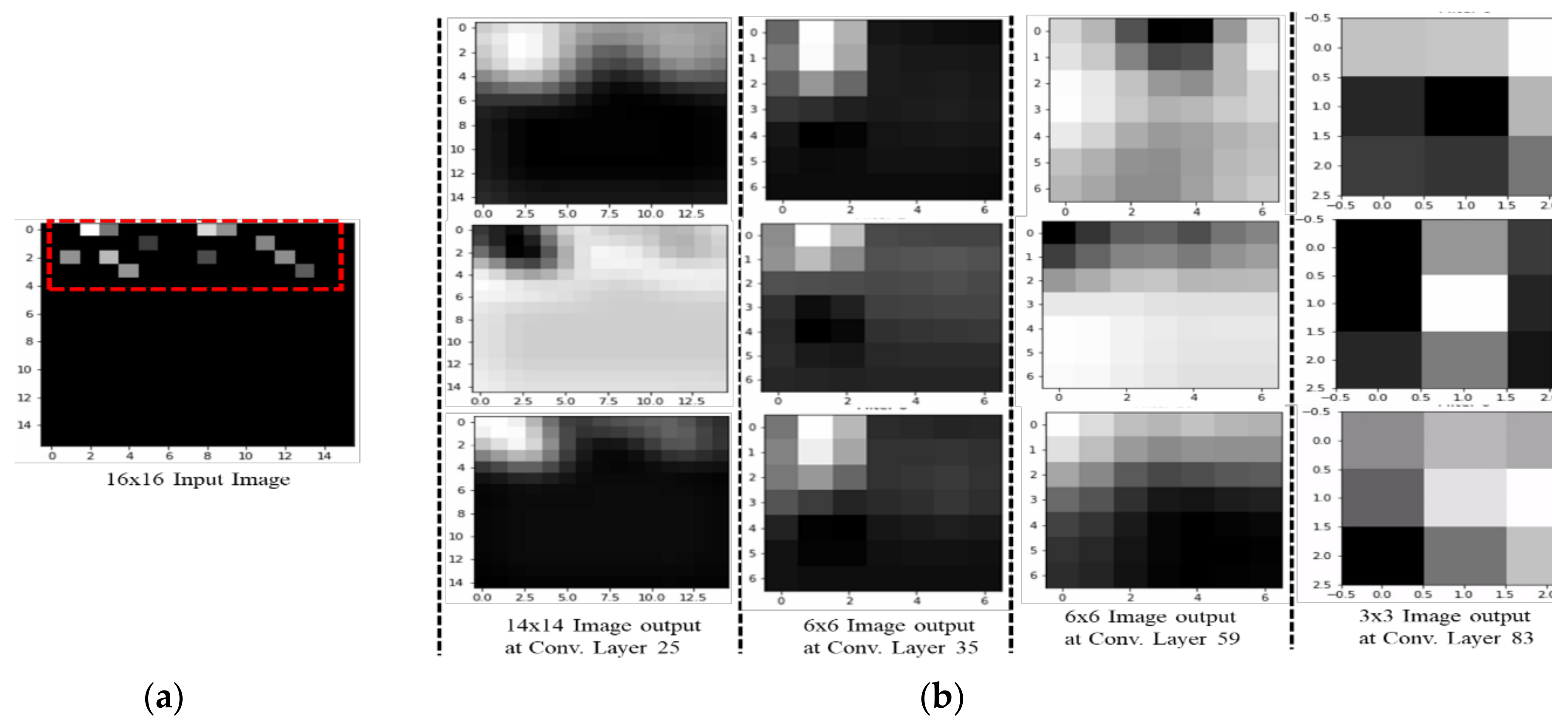
Another method to obtain higher classification accuracy is to widen the networks. Introduced in 2016, Inception v3 [44] is the combination of many ideas developed by several researchers. As shown in Figure 10, three modules are used to construct Inception v3. For inception module A in Figure 10a, two 3 × 3 convolutions replace a 5 × 5 convolution in the original inception module. For inception module B in Figure 10b, an n × 1 convolution followed by a 1 × n convolution replaces a 3 × 3 convolution (n = 3 in this paper). Inception module C increases the model width by dividing a 3 × 3 convolution into two 1 × 3 and 3 × 1 convolutions, shown in Figure 10c. With these inception modules, the number of parameters is reduced for the whole network to prevent overfitting. In Figure 11, a grid size reduction block is used to replace max pooling to increase network efficiency. Auxiliary classifiers were already suggested in a previous model of inception (i.e., Inception v1). There are some modifications in Inception-v3 (i.e., only one auxiliary classifier is used on the top of the last 17 × 17 layer, instead of using two auxiliary classifiers). Even though Inception v3 is deeper and wider than VGGNets, the computational cost and memory consumption of Inception v3 are much smaller than those of VGGNets. Figure 12 visualizes the activation of the 25th, 35th, 59th and 83rd convolutional network layers for Inception v3 in a 2D grid.
3.3.6. MobileNet v2
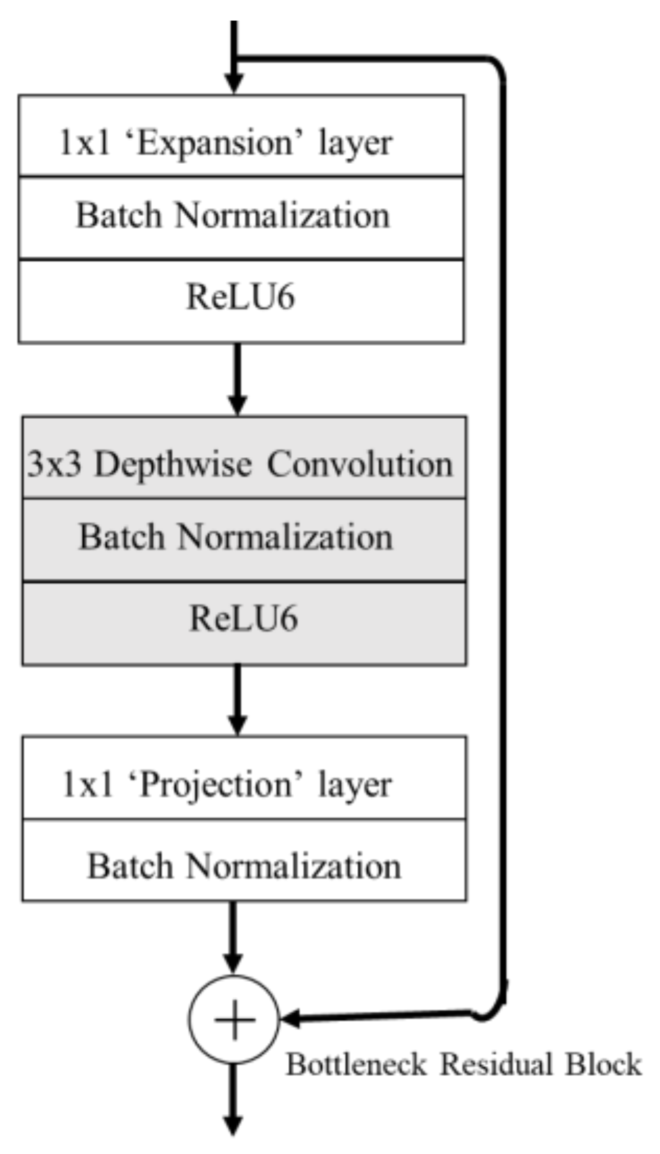
MobileNet v2 [45] uses a depthwise convolution layer in Figure 13. In the depthwise convolution layer, the number of input channels is equal to the number of filter channels. Using this layer keeps the total number of parameters at a minimum. The 1 × 1 convolution layer is the new layer introduced in the MobileNet v2 model, the purpose of which is to expand the number of channels in the data before it goes into the depthwise convolution. How much the data gets expanded is represented by the expansion factor, which is assumed to be ‘6’ in our work. The depthwise convolution layer is followed by a 1 × 1 convolution layer, named the pointwise/projection convolution layer. The projection layer projects the data with a high number of channels into output with a much lower number. The residual connection works like ResNet in helping MobileNet v2 to add the gradients. ReLU6 is used to prevent activations from happening too often. Figure 14 visualizes the activation of the 1st, 4th, 10th and 14th convolutional network layers for Inception v3 in a 2D grid.
4. Experiments and Results
4.1. Dataset and Experimental Setup
While the dataset collected during measurement was in a text format, the DL code was designed for a comma-separated values (CSV) input file. Given this, for training and testing, we converted the text files into a CSV file. These CSV files contained 257 columns and 74 RPs in the 257th column as labels. Data conversion was done using Python. The input for the file converter code (designed in Python) was folders containing text files.
To assess the validity of our approach, we created several datasets over four weeks. These were then used to assess which CNN layer is best to transfer knowledge from classification to indoor positioning as well as identifying the optimal classification algorithm. Results show that a relatively simple classification model fits the data well, producing ~95% generalization over a one-week period in the lab-based simulations with Scheme 1. The long-term introduction of new APs and drift in the existing APs need to be trained and learned.
To generate the dataset, the data is gathered over 7 days in four directions at the 74 RPs. It is then divided into four (Set 1: 7 days of data; Set 2: 5 days of data; Set 3: 3 days of data; and Set 4: 2 days of data), each then subdivided into separate cases based on the ratio of reference to trial data. For example, Set 1 (7 days of data) is divided into the three cases (6–1, 5–2 and 4–3). Datasets and cases are summarized in Table 3. The dataset with 7 days of data has the maximum number of input files; accordingly, it has better overall test accuracy than the other sets as shown in [11]. Therefore, Set 1/Case 1, which has six days of data for training and 1 day for testing, is used as the training and test dataset in our work.
RSSI fingerprint data collection and the final experiment were both performed on the 7th floor of the new engineering building at Dongguk University, Seoul, South Korea, shown in Figure 15.
4.2. Hyperparameter Settings
We trained the data on a network with different convolutional layers to find the best architecture. In each architecture, we adjusted the filter size, number of feature maps, pooling size, learning rate and batch size in the hyperparameter tuning process to retain the best configuration. We chose the best architecture with the best parameter setting as the final configuration. Table 4 shows the list of hyperparameters and their candidate values. The values in bold reflects the best hyperparameter setting for our CNN model.
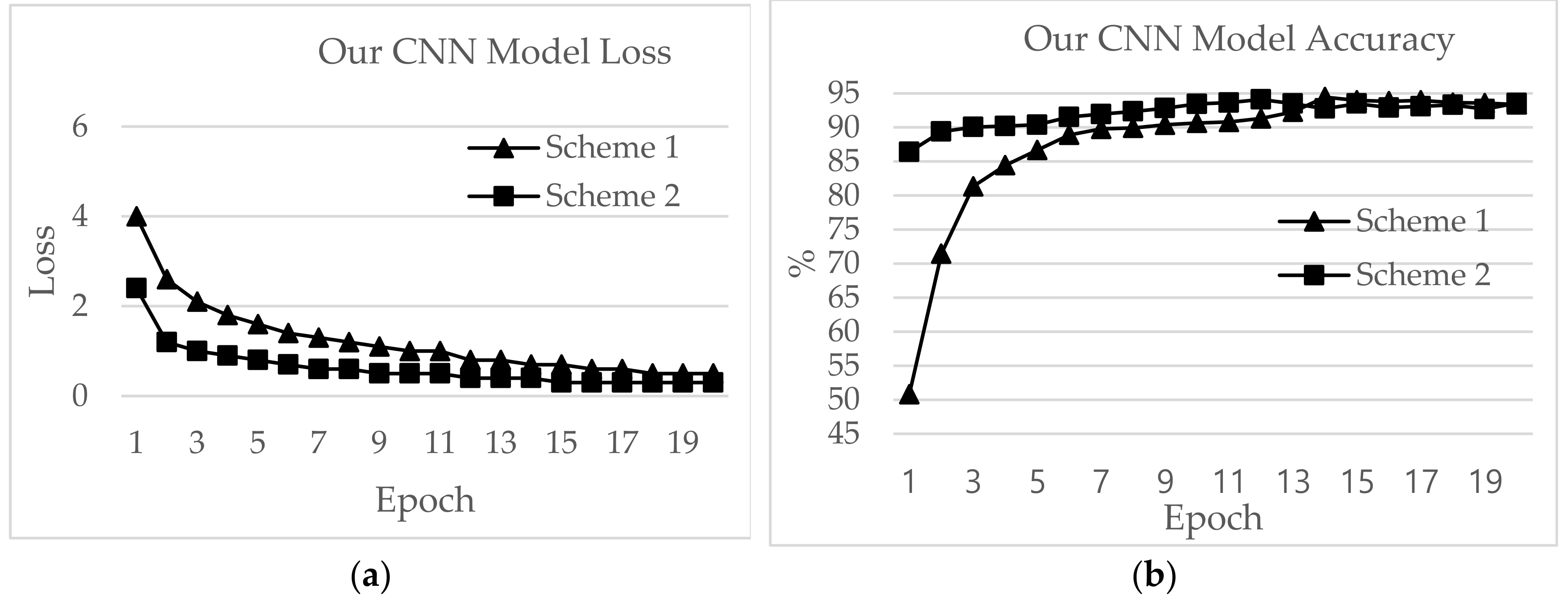
To analyse the effect of the number of layers, the CNN-based classifier was applied with different numbers of layers. The network with four convolutional layers outperformed others in all activities. The reason lies in the fact that networks with fewer than four convolutional layers are not complex enough to extract the appropriate features for activity recognition, whereas networks with four convolutional layers tend to cause over-fitting due to the structure complexity. Four convolutional layers are just enough to obtain good performance. The three-convolutional-layer network gives an accuracy of 91.32; however, the loss is higher compared to other layer networks. The loss in the setting signifies how well the CNN classifier learns from the training images to predict the test image correctly for each reference point. Therefore, lower losses are ideal for the CNN classifier. The test accuracy indicates how many test images are identified correctly by their own reference points or by a margin of 1 or 2 reference points. A higher test accuracy is desirable in accuracy of positioning case, since it reflects least error between training and testing environments. The epoch number is set to 20 due to the fact that the size of the dataset is few megabytes; therefore, with minimum epoch value model acquires high test accuracy. After 20–30 epochs, the model starts to overfit the result, and thus the total test accuracy start decreasing.
A seven-layer model has a test accuracy of 92.92% with loss 1.10 greater than a four-layer model. To determine the most appropriate filter size, the classifier was applied with different filter sizes (the number of convolutional layers was set to four). When the filter size was larger than three, the performance decreased with the increase of the filter size. The problem of overfitting occurs as filter size increases to seven and eleven. Therefore, the filter size was set to three. The best performance for each activity was achieved when the feature map was set to 64. The classification achieved the best performance when the pooling size was set to two. After this point, the performance decreased with the increase of the pooling size. Therefore, the pooling size was set to two. Table 4 shows that when the learning rate is less than 0.001, the algorithm achieves a steady and reliable performance, whereas a learning rate larger than 0.01 shows unstable results. The reason for the poor performance with a large learning rate is that the variables update too quickly to change to the proper gradient descent direction in a timely manner. However, a small learning rate with good performance is also not the best choice, because it results in a slow update of variables and leads to a slow training process. Therefore, the learning rate was set to 0.001. The activity increased as the batch size increased from 250 to 1000 and decreased as the batch size changed from 1000 to 2000. Therefore, the batch size was set to 1000. As shown in Table 4, the value in bold is the best setting of each hyperparameter.
All CNN applications require a different hyperparameter setting best suited for each application model. To determine the best parameter setting for our RSSI-based indoor localization problem, the CNN applications were performed by changing the learning rate and batch size. In Table 5, the value in bold is the best hyperparameter setting of each CNN application for RSSI-based positioning. The remaining hyperparameters of each application remained the same as their inbuilt by-default values.
The learning rate varied at 0.01, 0.001, 0.005 and 0.0001 with batch size 32, 64, 128 and 256, respectively. Once the CNN application achieves improved performance with a specific learning rate, then the batch size is altered for that learning rate. Hence, both parameters were set for each CNN application. For initial learning rate, the batch size is set to 32.
First, AlexNet performance is checked with the abovementioned learning rates. For learning rates 0.01 and 0.005, the loss values start with ~429 and remain the same after 20 epochs. At 0.0001, the initial loss value is 99.23 and test accuracy is highest, with 91.56% and loss value 79.85% after 5 epochs. At this learning rate, the batch size is varied, and batch size 64 achieved the highest test accuracy of 91.98%, for AlexNet. The optimum learning rate for ResNet is 0.0001 with initial loss value of 776.24, and after eight epochs the loss value is 212.98 with test accuracy 91.98%. At 0.005, the loss value reaches the highest at 12602.22, and test accuracy reduces to 6.79. At 0.0001 learning rate, batch size was tested for ResNet; batch size 32 produces the highest test accuracy of 89.74%, while batch size 256 produces ‘resource exhaust error’, which means the machine ran out of memory for allocating to the tensor. ZFNet gives the highest accuracy at 0.0001 learning rate, with a test accuracy of 91.71% and loss 46.76 after 5 epochs. The best-suited batch size for ZFNet is 64, with a test accuracy of 91.72%. In Inception v3 and MobileNet v2 the learning rate remained at 0.001. The total number of convolution layers in Inception v3 is 99, while in MobileNet v2 it is 56 (including the inverted residual blocks). Therefore, changing the learning rate exhausts the memory of the machine. The batch size for Inception v3 is 64 with a test accuracy of 87.09% at the 5th epoch, because the remaining batch size has overfitting results. For MobileNet v2, batch size 64 produces the highest test accuracy, with 88.54% and loss of 13.26 at the 3rd epoch. The initial loss value for MobileNet is 24.36.
4.3. Comparison with Other CNN Classification Methods
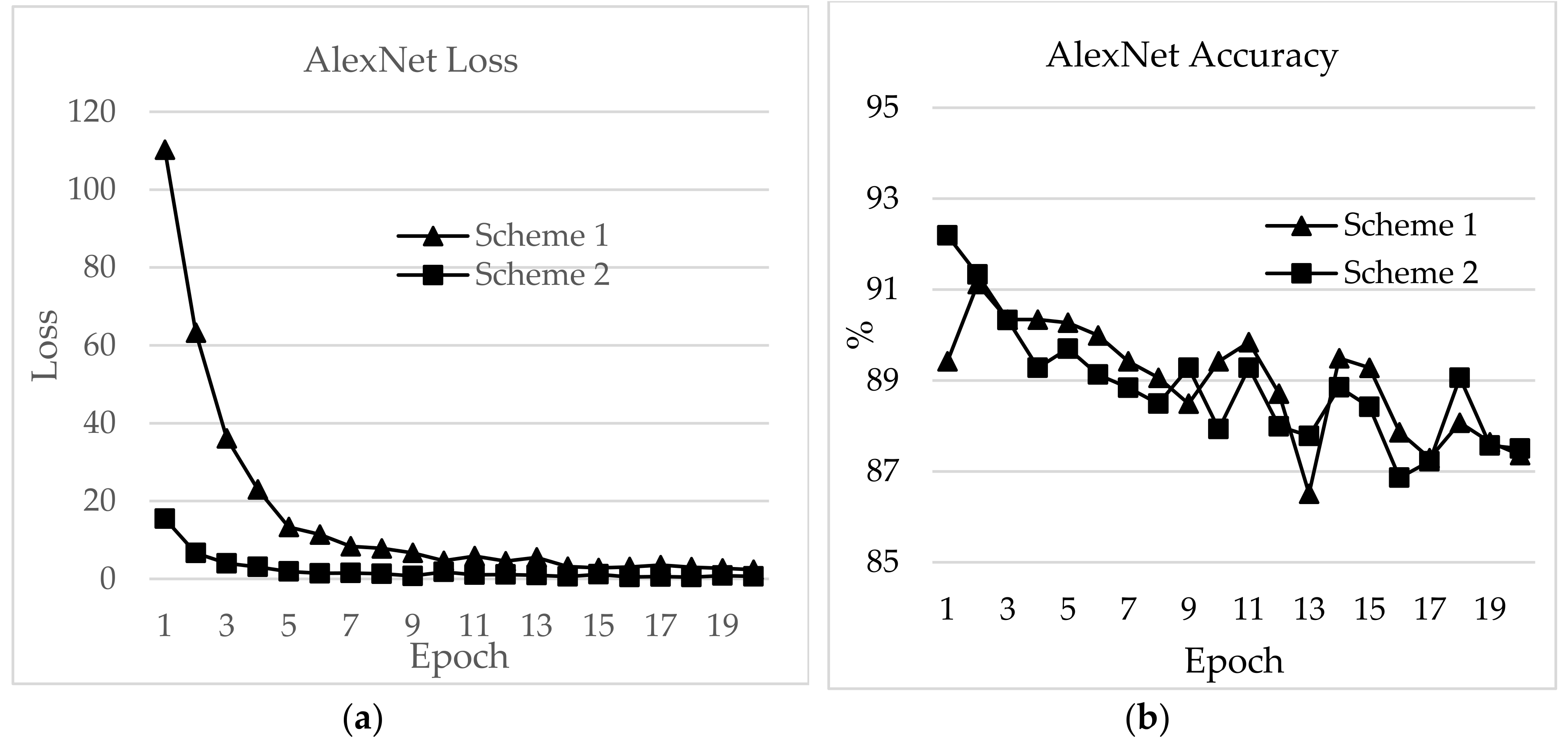
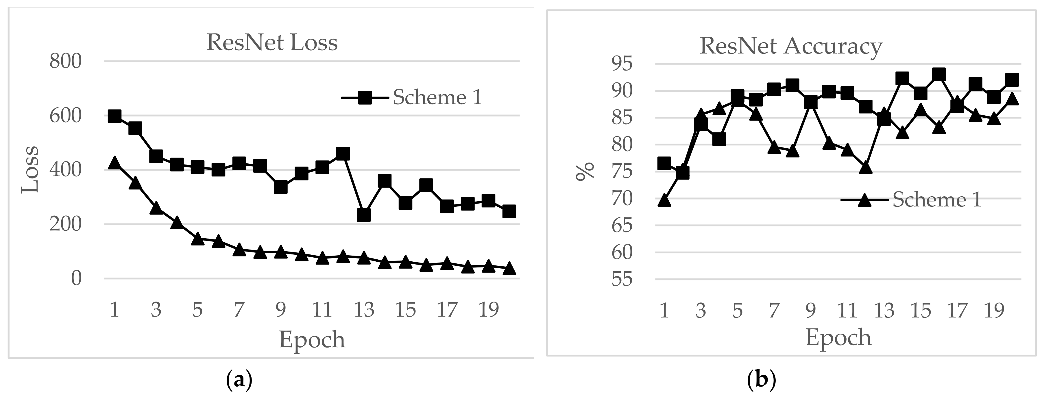
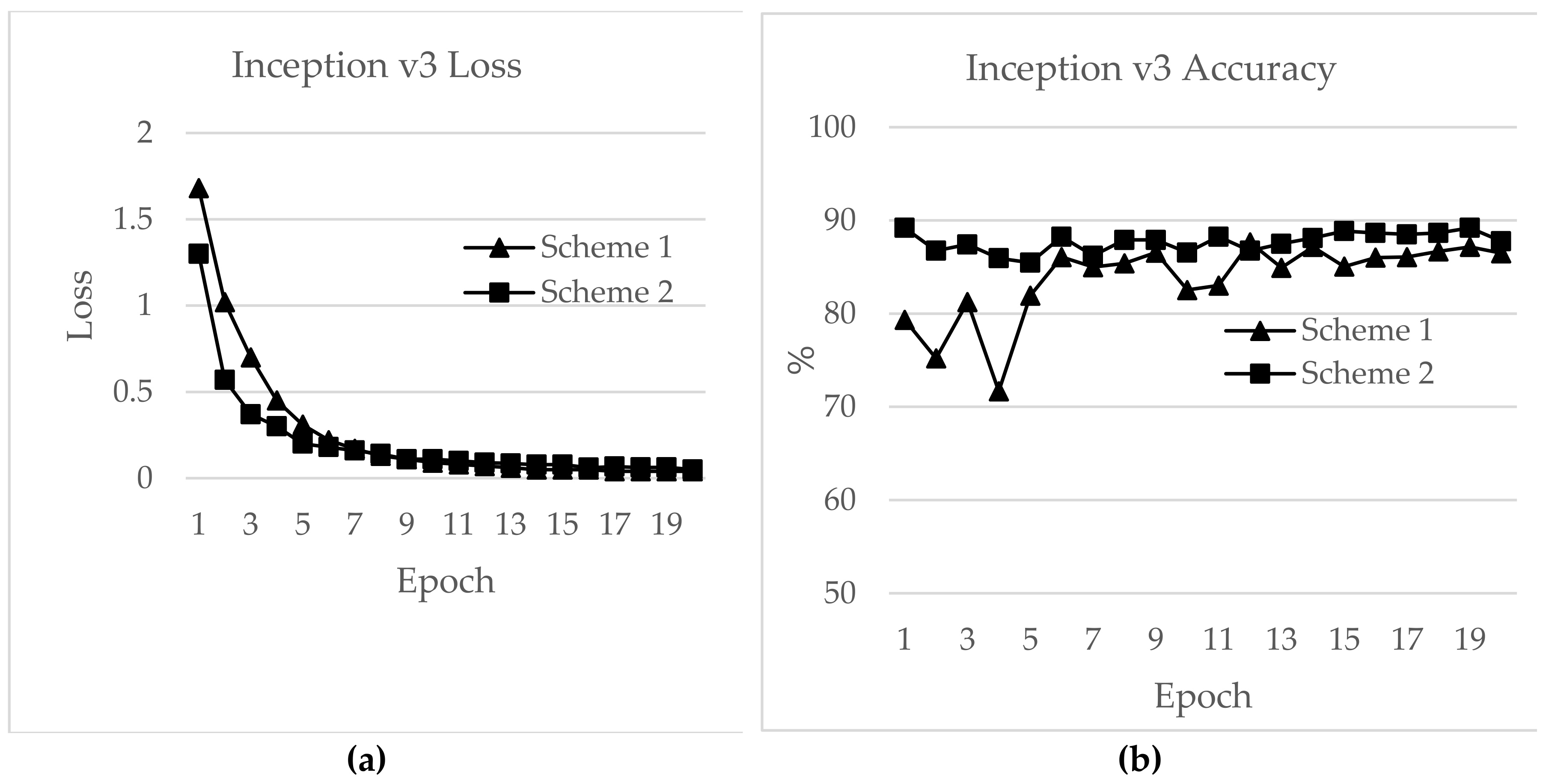
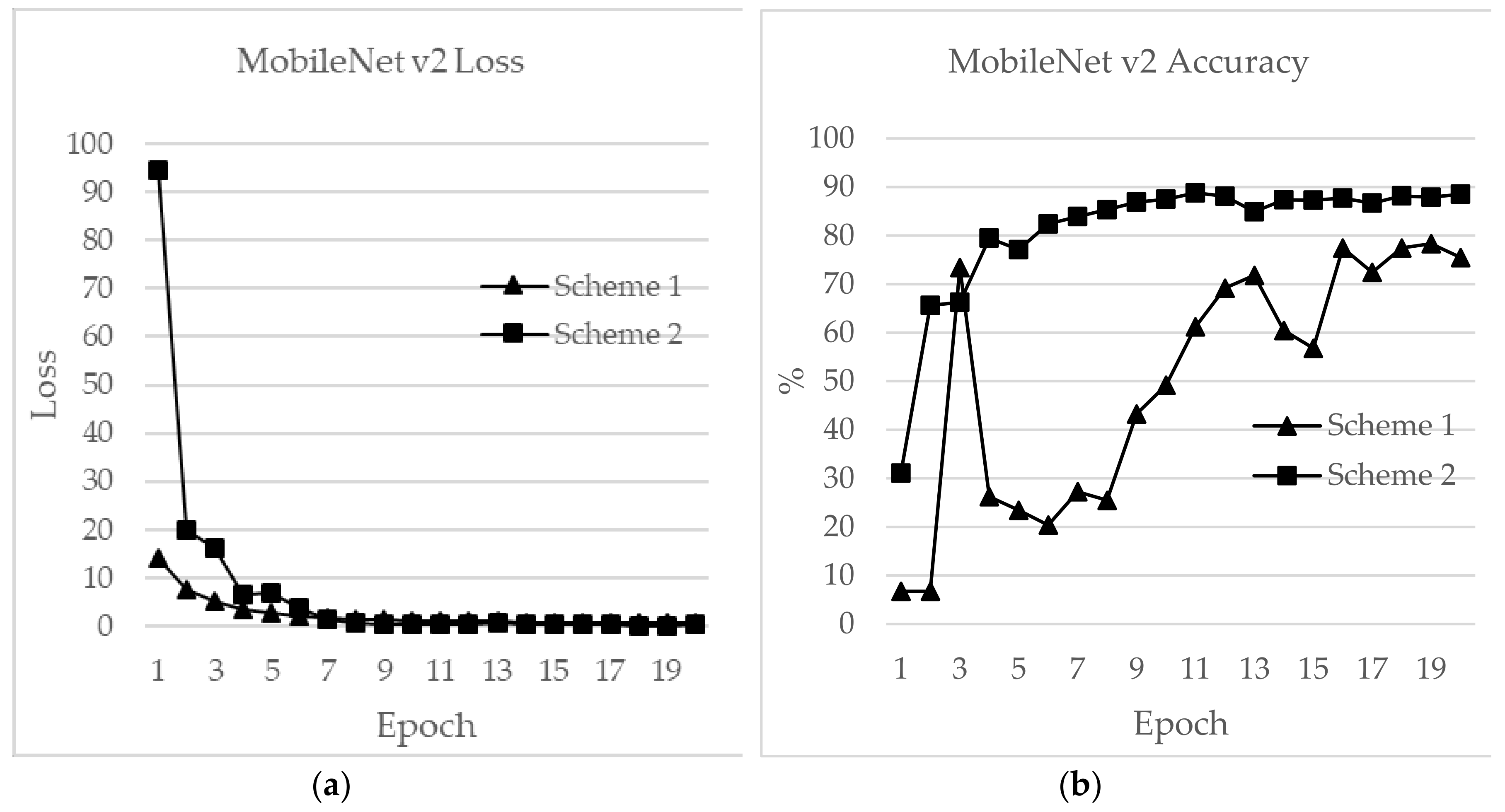
In this section, a detailed analysis of RSSI-based dataset localization performance is presented. To evaluate the performance of the prevailing CNNs, we investigated four aspects: validation accuracy, test accuracy, loss and time for each epoch. The accuracy curves for different CNN applications are shown in Figure 16, Figure 17, Figure 18, Figure 19, Figure 20 and Figure 21. As presented in Figure 17, the features extracted from AlexNet are similar to the observation for the RSSI dataset. In Figure 17, the loss for AlexNet is shown for both schemes. The initial loss and accuracy values were 110.29 and 89.42%, respectively, for Scheme 1 and 15.46 and 92.19%, respectively, for Scheme 2. AlexNet achieved a maximum accuracy of 91.12% for Scheme 1 and 91.19% for Scheme 2. This means that the network is well-suited as an RSSI-type fingerprinting dataset. The minimum loss values after 20 epochs were 2.37 and 0.66 for Schemes 1 and 2, respectively. As presented in Figure 18, ResNet showed a maximum accuracy of 88.57% for Scheme 1 and 93.00% for Scheme 2. However, the losses after 20 epochs were 246.70 and 50.1 for Schemes 1 and 2, respectively. The accuracy further decreased even after the decrease of loss values. Therefore, the highest value reported for the ResNet model was the optimum value for RSSI-type datasets. The initial accuracy values for ResNet for Schemes 1 and 2 were 69.74% and 76.49%, respectively, and the losses were 596.81 and 427.04, respectively. As shown in Figure 19, due to its simple architecture similar to AlexNet, ZFNet performed well for the RSSI dataset. Both training and testing showed accuracy values above 90%. The initial and highest accuracy values for ZFNet for Schemes 1 and 2 were 90.84% and 92.05%, respectively, with losses of 99.05 and 13.52, respectively. The accuracies after 20 epochs were 86.29% and 87.71%, with a loss of 1.76 and 0.48, respectively. Inception v3 was the lengthiest network to be trained and tested for the RSSI data type. As shown in Figure 20, surprisingly, the highest accuracies achieved for this network for Schemes 1 and 2 were 87.16% and 89.20%, respectively. The loss values were 0.04 for Scheme 1 and 0.063 for Scheme 2. The initial loss values were 1.68 and 1.3 with accuracies of 79.35% and 89.02%, respectively. The final loss and accuracy values for Inception v3 after 20 epochs were 0.04 and 86.48%, respectively, for Scheme 1 and 0.05 and 87.77%, respectively, for Scheme 2. Figure 21 shows loss and accuracy for MobileNet v2. MobileNet v2 achieved the highest accuracy of 88.52%, for Scheme 2 and 78.33% for Scheme 1, which showed the lowest accuracy among the CNN applications. The initial and final loss values for MobileNet v2 were 19.95 and 0.6, respectively, for Scheme 1 and 94.45 and 0.25, respectively, for Scheme 2.
A performance comparison of a CNN application on the basis of four aspects was performed for the above models. As shown in Table 6, our CNN model outperformed other applications in comparisons of epoch time, loss, validation and test accuracy.
The highest test accuracy achieved by our CNN model was 94.45% for the loss value of 0.7 with Scheme 1. Scheme 2 performed similarly, with a test accuracy of 94.11 and loss of 0.4. The epoch time was ~2 seconds for Scheme 1 and ~8 seconds for Scheme 2. The training accuracies were 69.87% and 86.99% for Schemes 1 and 2, respectively.
The second highest test accuracy was achieved by ResNet, with 93.00% for Scheme 2. The training accuracy was 96.44%. However, the epoch time was as high as 44.39 min while the loss was 56.54 for Scheme 2. For Scheme 1, the training accuracy was 81.88% and the test accuracy was 88.57%.
AlexNet performed best in terms of epoch time, with 1.41 and 6.78 min for Schemes 1 and 2, respectively, and test accuracies of 91.12% and 92.19%, respectively. The test accuracies for ZFNet were 90.83% and 92.05%, and the epoch times were 3.54 and 16.47 min for Schemes 1 and 2, respectively. The lowest test accuracy was exhibited by Inception v3, with 87.64% for Scheme 1 and 89.20% for Scheme 2. The epoch times for Schemes 1 and 2 were 4.17 and 20.38 minutes, and the training accuracies were 97.68% and 91.52%, respectively. MobileNet v2 showed epoch times of 4.15 min and 20.32 min with test accuracies of 78.33% and 88.52% for Schemes 1 and 2, respectively.
As shown in Table 7, the number of RPs predicted accurately by the applications was called the zero-margin accuracy. Our CNN model had the highest zero-margin prediction, with 45.43% and 46.54% accuracy for Schemes 1 and 2, respectively. A two-meter difference between the actual and predicted RP was termed the one-margin accuracy. Our CNN model and ZFNet had similar outcomes, with 52.63% and 52.34% one-margin accuracy, respectively, for Scheme 1 and 51.23% and 51.14%, respectively, for Scheme 2. A difference of four meters between the predicted and actual outputs was called the two-margin accuracy. The highest two-margin accuracy was shown by our CNN model, with 94.45% and 94.11% for Schemes 1 and 2, respectively. The lowest two-margin accuracy was shown by MobileNet v2, with 78.33% and 88.52% for Schemes 1 and 2, respectively.
An indoor localization system is best evaluated on the basis of performance statistics using the mean value, variations and standard deviation. The mean is the total number of errors in meter units for indoor localization and is best if closest to zero. As shown in Table 8, our CNN model achieved mean errors as low as 1.44 m and 1.48 m for Schemes 1 and 2, respectively, with standard deviations of 2.12 m and 2.35 m, respectively. AlexNet performed the best among the other CNN applications, with means of 1.80 and 1.67 m and standard deviations of 2.42 and 2.55 m for Schemes 1 and 2, respectively. Inception v3 showed mean errors of 4.39 and 4.23 m, standard deviations of 8.19 and 7.57 m and variations of 67.06 and 57.34 m for Schemes 1 and 2, respectively. The highest mean error is shown by MobileNet v2, with 4.39 m and 4.23 m and standard deviations 8.19 m and 7.57 m for Schemes 1 and 2, respectively.
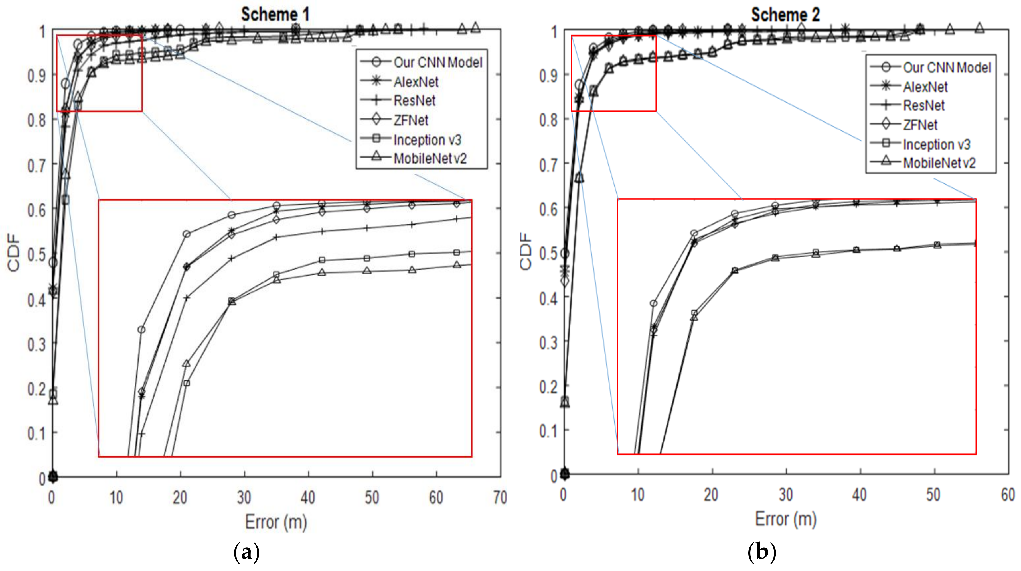
We also evaluated the effectiveness of indoor positioning (i.e., positioning accuracy), defined as the cumulative percentage of location error within a specified distance (Figure 22). Our CNN model outperformed the other CNN applications over the entire range of the graph. Our CNN model with Schemes 1 and 2 did not differ greatly by positioning accuracy, such as in cases with error distance <5 m. Both schemes had probability values above 94% within <5 m error distance. However, for cumulative distribution functions over 94%, the positioning accuracy of Scheme 1 fell behind that of Scheme 2. Under 94%, the error distance for our CNN model was approximately 1.44 m, and Scheme 1 is ~0.03 m more accurate than Scheme 2. The gap between the two schemes increased gradually, and the error distance eventually rose to nearly 38 m. AlexNet and ZFNet achieved a probability of 91% within a 5-m error distance. Both had an error distance of 1.8 meters from the beginning and end of the graph with Scheme 1. ResNet lagged behind, with an error distance of 2.44 m and an accuracy of 88.57%. The gap eventually increased, and the error distance rose to 18 m for AlexNet, 26 m for ZFNet and 58 m for ResNet, which is the maximum value. Inception v3 had a maximum error distance of 4.13 m and 87.64% position accuracy within 5 m. The error distance for Inception v3 eventually increased to 54 m. With Scheme 2, the distance errors for AlexNet, ResNet and ZFNet became 1.7 m with ~92% accuracy for cumulative distribution functions. Therefore, the graphs for these models overlapped. The error distance eventually increased after 5 m. The error distance for AlexNet increased to 38 m, while that for ZFNet increased to 32 m. ResNet outperformed both models, with an error distance of up to 48 m. Inception v3 had an error distance of 4.10 m with an accuracy of 89.66%. After 5 m, the error distance for Inception v3 with Scheme 2 increased to 48 m. MobileNet v2 showed an error distance of 4.39 m with an accuracy of 78.38% for Scheme 1 and 4.23 m with 88.52% for Scheme 2.
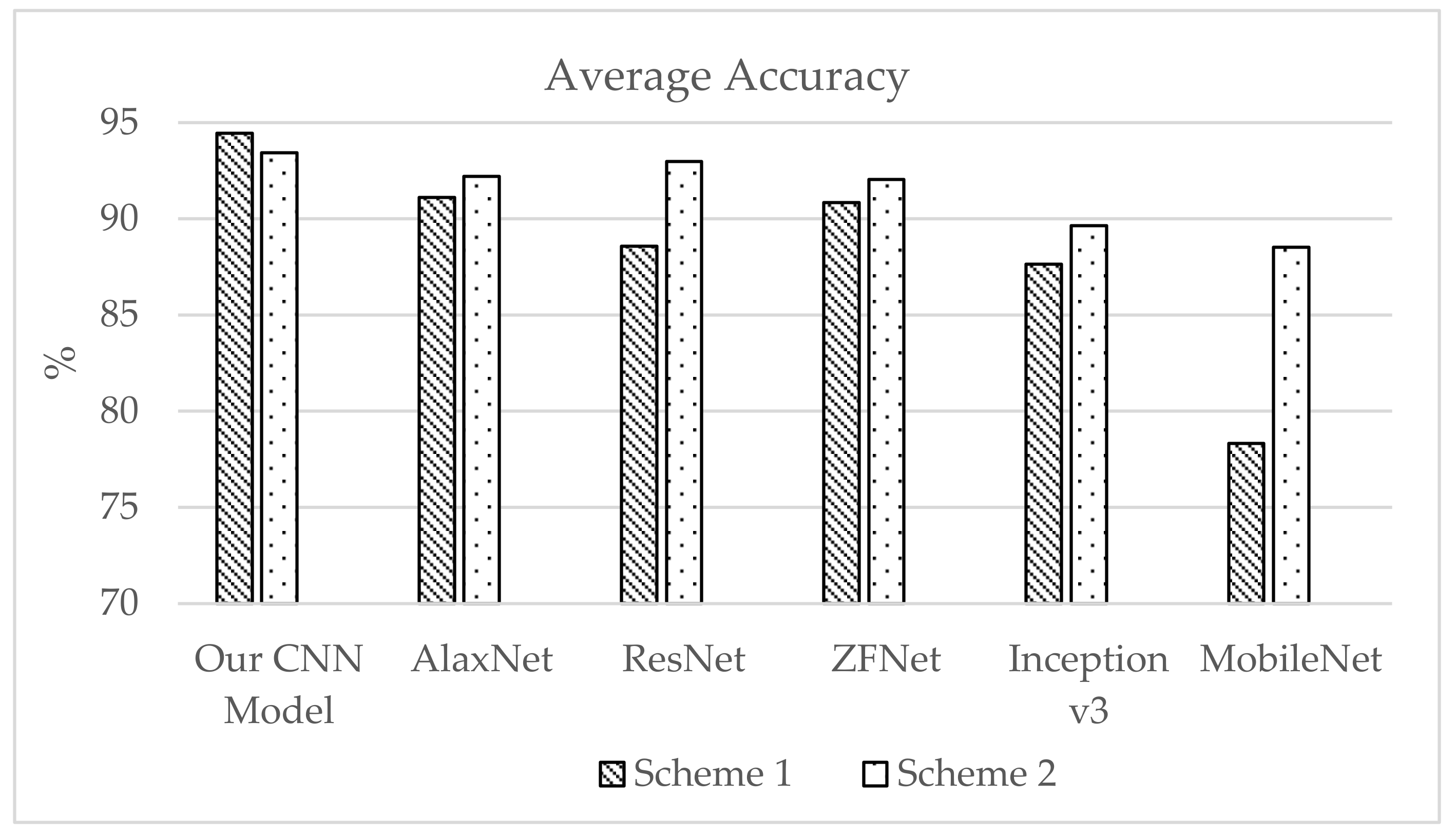
Figure 23 presents the average test accuracy with two lab test simulation results. Scheme 2 performed better with all CNN applications. The localization techniques proposed with our CNN model provide higher accuracy overall (i.e., a smaller error). We observed that CNN can fully exploit the additional measurements, making it a promising technique for environments with a high density of APs. In addition to the improved performance, our CNN model provides a fingerprinting approach that requires a less laborious offline calibration phase.
5. Conclusions
This paper presents a novel approach to indoor localization that is proven sufficiently efficient to achieve a low error distance with high test accuracy. In this study, we developed a CNN model for a DL scheme for Wi-Fi-based localization. In the offline stage of DL, a four-layer CNN structure is trained to extract features from fluctuating Wi-Fi signals and to build fingerprints. In the online positioning stage, the proposed CNN-based localizer estimates the position of the target. Our CNN model was compared with five CNN applications: AlexNet, ResNet, ZFNet, Inception v3 and MobileNet v2. Each application achieved a maximum simulation success rate of ~90%, while our CNN model achieved a success rate of 94%. This indicates that the proposed CNN model can better handle the instability and variability of RSSIs for Wi-Fi signals in complex indoor environments. This means it is more powerful in classification tasks in fingerprint indoor positioning. Future research will expand our CNN model and CNN applications for testing under real-time environments to work seamlessly through indoor positioning systems and compare the output of each model. We can then identify the best-performing CNN model for indoor positioning systems.
Author Contributions
R.S.S. and S.-H.H. contributed to the main idea of this research. R.S.S. wrote the computation codes, performed the simulations, experiments, and database collection. The research activity was planned and executed under the supervision of S.-H.H. R.S.S. and S.-H.H. contributed to the writing of this article.
Funding
This research received no external funding.
Acknowledgments
The authors would like to offer their sincere gratitude to Sang Moon Lee, CTO of JMP Systems, Korea, for providing the equipment for database collection and setting up the experimental environment.
Conflicts of Interest
The authors declare no conflict of interests regarding the publication of this article.
References
- Wu, S.; Chen, T.; Wu, Y.; Lytras, M. Smart cities in Taiwan: A perspective on big data applications. Sustainability 2018, 10, 106. [Google Scholar] [CrossRef]
- Mier, J.; Jaramillo-Alcázar, A.; Freire, J.J. At a Glance: Indoor Positioning Systems Technologies and Their Applications Areas. In Advances in Intelligent Systems and Computing, Proceedings of the International Conference on Information Technology & Systems, Quito, Ecuador, 6–8 February 2019; Springer: Cham, Switzerland, 2019; pp. 483–493. [Google Scholar]
- Youssef, M.; Agrawala, A. The Horus WLAN location determination system. In Proceedings of the International Conference on Mobile Systems, Applications, and Services, Seattle, WA, USA, 6–8 June 2005; pp. 205–218. [Google Scholar]
- Perera, C.; Aghaee, S.; Faragher, R.; Harle, R.; Blackwell, A.F. Contextual Location in the Home using Bluetooth Beacons. IEEE Syst. J. 2018, 20, 2720–2723. [Google Scholar] [CrossRef]
- Liu, T.; Shuai, Z. Self-Positioning System and Algorithm in Wireless Sensor Networks. In Proceedings of the 2018 3rd International Workshop on Materials Engineering and Computer Sciences (IWMECS 2018), Jinan, China, 27–28 January 2018. [Google Scholar] [CrossRef]
- Choosaksakunwiboon, S.; Terawong, C.; Suttisirikul, S.; Anantavrasilp, I.; Thiemjarus, S.; Wisadsud, S.; Kaemarungsi, K. A Pre-processing Technique for BLE-based Indoor Localization. In Proceedings of the 12th International Convention on Rehabilitation Engineering and Assistive Technology, Shanghai, China, 13–16 July 2018; Therapeutic, Assistive & Rehabilitative Technologies (START) Centre: Singapore, 2018; pp. 241–244. [Google Scholar]
- Gomes, A.; Pinto, A.; Soares, C.; Torres, J.M.; Sobral, P.; Moreira, R.S. Indoor Location Using Bluetooth Low Energy Beacons. In Advances in Intelligent Systems and Computing, Proceedings of the World Conference on Information Systems and Technologies, Galicia, Spain, 16–19 April 2018; Springer: Cham, Switzerland, 2018; pp. 565–580. [Google Scholar]
- Mittal, A.; Tiku, S.; Pasricha, S. Adapting convolutional neural networks for indoor localization with smart mobile devices. In Proceedings of the 2018 on Great Lakes Symposium on VLSI, Chicago, IL, USA, 23–25 May 2018; pp. 117–122. [Google Scholar]
- Zafari, F.; Gkelias, A.; Leung, K.K. A survey of indoor localization systems and technologies. IEEE Commun. Surv. Tutor. 2019, 21, 2568–2599. [Google Scholar] [CrossRef]
- Chishti, S.O.; Riaz, S.; Bilal Zaib, M.; Nauman, M. Self-Driving Cars Using CNN and Q-Learning. In Proceedings of the 2018 IEEE 21st International Multi-Topic Conference (INMIC), Karachi, Pakistan, 1–2 December 2018; pp. 1–7. [Google Scholar]
- Sinha, R.S.; Lee, S.-M.; Rim, M.; Hwang, S.-H. Data Augmentation Schemes for Deep Learning in an Indoor Positioning Application. Electronics 2019, 8, 554. [Google Scholar] [CrossRef]
- Hattori, K.; Tatebe, N.; Kagawa, T.; Owada, Y.; Shan, L.; Temma, K.; Hamaguchi, K.; Takadama, K. Deployment of wireless mesh network using RSSI-based swarm robots. Artif. Life Robot. 2016, 21, 434–442. [Google Scholar] [CrossRef]
- Neburka, J.; Tlamsa, Z.; Benes, V.; Polak, L.; Kaller, O.; Bolecek, L.; Sebesta, J.; Kratochvil, T. Study of the performance of RSSI based Bluetooth Smart indoor positioning. In Proceedings of the 2016 26th International Conference Radioelektronika (RADIOELEKTRONIKA), Kosice, Slovakia, 19–20 April 2016; pp. 121–125. [Google Scholar]
- Wang, Y.; Ye, Q.; Cheng, J.; Wang, L. RSSI-based bluetooth indoor localization. In Proceedings of the 2015 11th International Conference on Mobile Ad-hoc and Sensor Networks (MSN), Shenzhen, China, 16–18 December 2015; pp. 165–171. [Google Scholar]
- Zhang, S.; Guo, J.; Luo, N.; Wang, L.; Wang, W.; Wen, K. Improving Wi-Fi Fingerprint Positioning with a Pose Recognition-Assisted SVM Algorithm. Remote Sens. 2019, 11, 652. [Google Scholar] [CrossRef]
- Jang, B.; Kim, H. Indoor Positioning Technologies Without Offline Fingerprinting Map: A Survey. IEEE Commun. Surv. Tutor. 2018, 21, 508–525. [Google Scholar] [CrossRef]
- Guan, R.; Harle, R. Signal Fingerprint Anomaly Detection for Probabilistic Indoor Positioning. In Proceedings of the 2018 International Conference on Indoor Positioning and Indoor Navigation (IPIN), Nantes, France, 24–27 September 2018; pp. 1–8. [Google Scholar]
- Mendoza-Silva, G.; Richter, P.; Torres-Sospedra, J.; Lohan, E.; Huerta, J. Long-term WiFi fingerprinting dataset for research on robust indoor positioning. Data 2018, 3, 3. [Google Scholar] [CrossRef]
- Li, G.; Geng, E.; Ye, Z.; Xu, Y.; Lin, J.; Pang, Y. Indoor positioning algorithm based on the improved RSSI distance model. Sensors 2018, 18, 2820. [Google Scholar] [CrossRef]
- Kim, K.S.; Lee, S.; Huang, K. A scalable deep neural network architecture for multi-building and multi-floor indoor localization based on Wi-Fi fingerprinting. Big Data Anal. 2018, 3, 4. [Google Scholar] [CrossRef] [Green Version]
- Hsieh, H.-Y.; Prakosa, S.W.; Leu, J.-S. Towards the Implementation of Recurrent Neural Network Schemes for WiFi Fingerprint-Based Indoor Positioning. In Proceedings of the 2018 IEEE 88th Vehicular Technology Conference (VTC-Fall), Chicago, IL, USA, 27–30 August 2018; pp. 1–5. [Google Scholar]
- Wang, R.; Li, Z.; Luo, H.; Zhao, F.; Shao, W.; Wang, Q. A Robust Wi-Fi Fingerprint Positioning Algorithm Using Stacked Denoising Autoencoder and Multi-Layer Perceptron. Remote Sens. 2019, 11, 1293. [Google Scholar] [CrossRef]
- Le, D.V.; Meratnia, N.; Havinga, P.J.M. Unsupervised Deep Feature Learning to Reduce the Collection of Fingerprints for Indoor Localization Using Deep Belief Networks. In Proceedings of the 2018 International Conference on Indoor Positioning and Indoor Navigation (IPIN), Nantes, France, 24–27 September 2018; pp. 1–7. [Google Scholar]
- Dai, P.; Yang, Y.; Wang, M.; Yan, R. Combination of DNN and Improved KNN for Indoor Location Fingerprinting. Wirel. Commun. Mob. Comput. 2019, 2019, 9. [Google Scholar] [CrossRef]
- Cheng, C.-H.; Yan, Y. Indoor positioning system for wireless sensor networks based on two-stage fuzzy inference. Int. J. Distrib. Sens. Netw. 2018, 14, 1550147718780649. [Google Scholar] [CrossRef]
- Adege, A.; Lin, H.-P.; Tarekegn, G.; Jeng, S. Applying deep neural network (DNN) for robust indoor localization in multi-building environment. Appl. Sci. 2018, 8, 1062. [Google Scholar] [CrossRef]
- Sun, W.; Xue, M.; Yu, H.; Tang, H.; Lin, A. Augmentation of Fingerprints for Indoor WiFi Localization Based on Gaussian Process Regression. IEEE Trans. Veh. Technol. 2018, 67, 10896–10905. [Google Scholar] [CrossRef]
- Wei, Y.; Hwang, S.-H.; Lee, S.-M. IoT-Aided Fingerprint Indoor Positioning Using Support Vector Classification. In Proceedings of the 2018 International Conference on Information and Communication Technology Convergence (ICTC), Jeju, Korea, 17–19 October 2018; pp. 973–975. [Google Scholar]
- Xu, H.; Wu, M.; Li, P.; Zhu, F.; Wang, R. An RFID indoor positioning algorithm based on support vector regression. Sensors 2018, 18, 1504. [Google Scholar] [CrossRef] [PubMed]
- Jang, J.-W.; Hong, S.-N. Indoor Localization with WiFi Fingerprinting Using Convolutional Neural Network. In Proceedings of the 2018 Tenth International Conference on Ubiquitous and Future Networks (ICUFN), Prague, Czech Republic, 3–6 July 2018; pp. 753–758. [Google Scholar]
- Niitsoo, A.; Edelhäußer, T.; Eberlein, E.; Hadaschik, N.; Mutschler, C. A Deep Learning Approach to Position Estimation from Channel Impulse Responses. Sensors 2019, 19, 1064. [Google Scholar] [CrossRef] [PubMed]
- Wang, X.; Gao, L.; Mao, S.; Pandey, S. CSI-based fingerprinting for indoor localization: A deep learning approach. IEEE Trans. Veh. Technol. 2016, 66, 763–776. [Google Scholar] [CrossRef]
- Won, M.; Sahu, S.; Park, K.-J. DeepWiTraffic: Low Cost WiFi-Based Traffic Monitoring System Using Deep Learning. arXiv 2018, arXiv:1812.08208. [Google Scholar]
- Jia, Y.; Shelhamer, E.; Donahue, J.; Karayev, S.; Long, J.; Girshick, R.; Guadarrama, S.; Darrell, T. Caffe: Convolutional architecture for fast feature embedding. In Proceedings of the 22nd ACM international conference on Multimedia, Orlando, FL, USA, 3–7 November 2014; pp. 675–678. [Google Scholar]
- Li, H.; Ota, K.; Dong, M.; Guo, M. Learning human activities through Wi-Fi channel state information with multiple access points. IEEE Commun. Mag. 2018, 56, 124–129. [Google Scholar] [CrossRef]
- Xiao, H.; Rasul, K.; Vollgraf, R. Fashion-mnist: a novel image dataset for benchmarking machine learning algorithms. arXiv 2017, arXiv:1708.07747. [Google Scholar]
- Zhou, B.; Yang, J.; Li, Q. Smartphone-Based Activity Recognition for Indoor Localization Using a Convolutional Neural Network. Sensors 2019, 19, 621. [Google Scholar] [CrossRef] [PubMed]
- Valada, A.; Radwan, N.; Burgard, W. Deep auxiliary learning for visual localization and odometry. In Proceedings of the 2018 IEEE International Conference on Robotics and Automation (ICRA), Brisbane, QLD, Australia, 21–25 May 2018; pp. 6939–6946. [Google Scholar]
- Hanni, A.; Chickerur, S.; Bidari, I. Deep learning framework for scene based indoor location recognition. In Proceedings of the 2017 International Conference on Technological Advancements in Power and Energy (TAP Energy), Kollam, India, 21–23 December 2017; pp. 1–8. [Google Scholar]
- Maisano, R.; Tomaselli, V.; Capra, A.; Longo, F.; Puliafito, A. Reducing Complexity of 3D Indoor Object Detection. In Proceedings of the 2018 IEEE 4th International Forum on Research and Technology for Society and Industry (RTSI), Palermo, Italy, 10–13 September 2018; pp. 1–6. [Google Scholar]
- Jia, Y.; Shelhamer, E.; Donahue, J.; Karayev, S.; Long, J.; Girshick, R.; Guadarrama, S.; Darrell, T. Caffe: Convolutional architecture for fast feature embedding. In Proceedings of the 22nd ACM international conference on Multimedia, Orlando, Florida, USA, 3–7 November 2014; pp. 675–678. [Google Scholar]
- He, K.; Zhang, X.; Ren, S.; Sun, J. Deep residual learning for image recognition. In Proceedings of the IEEE Conference on Computer Vision and Pattern Recognition, Las Vegas, NV, USA, 27–30 June 2016; pp. 770–778. [Google Scholar]
- Zeiler, M.D.; Fergus, R. Visualizing and understanding convolutional networks. In Lecture Notes in Computer Science, Proceedings of the European Conference on Computer Vision, Zurich, Switzerland, 6–12 September 2014; Springer: Cham, Switzerland, 2014; pp. 818–833. [Google Scholar]
- Szegedy, C.; Vanhoucke, V.; Ioffe, S.; Shlens, J.; Wojna, Z. Rethinking the inception architecture for computer vision. In Proceedings of the IEEE Conference on Computer Vision and Pattern Recognition, Las Vegas, NV, USA, 27–30 June 2016; pp. 2818–2826. [Google Scholar]
- Sandler, M.; Howard, A.; Zhu, M.; Zhmoginov, A.; Chen, L.-C. Mobilenetv2: Inverted residuals and linear bottlenecks. In Proceedings of the IEEE Conference on Computer Vision and Pattern Recognition, Salt Lake City, UT, USA, 18–23 June 2018; pp. 4510–4520. [Google Scholar]
Figure 1.
Deep learning input file conversion from 256 received signal strength indicator (RSSI) values to a 16 × 16 image. (a) Input comma-separated values (CSV) readings of the nine visible RSSIs from a total of 256 access points (APs). (b) Converted grayscale image with nine bright spots representing APs visible at the reference point (RP) [11].

Figure 2.
Proposed convolutional neural network (CNN) architecture for the indoor Wi-Fi positioning system in this study.
Figure 2.
Proposed convolutional neural network (CNN) architecture for the indoor Wi-Fi positioning system in this study.

Figure 3.
Images for our CNN model. (a) Input image. (b) Output image with different convolutional layers.
Figure 3.
Images for our CNN model. (a) Input image. (b) Output image with different convolutional layers.

Figure 4.
The architecture of AlexNet [38].
Figure 4.
The architecture of AlexNet [38].

Figure 5.
Images for AlaxNet. (a) Input image. (b) Output image with different convolutional layers.
Figure 5.
Images for AlaxNet. (a) Input image. (b) Output image with different convolutional layers.

Figure 6.
The architecture of ResNet [41].
Figure 6.
The architecture of ResNet [41].

Figure 7.
Images for ResNet. (a) Input image. (b) Output image with different convolutional layer.

Figure 8.
The architecture of ZFNet [43].
Figure 8.
The architecture of ZFNet [43].

Figure 9.
Images for ZFNet. (a) Input image. (b) Output image with different convolutional layer.

Figure 10.
The architecture of inception module. (a) Inception module A, (b) Inception module B and (c) Inception module C.
Figure 10.
The architecture of inception module. (a) Inception module A, (b) Inception module B and (c) Inception module C.

Figure 11.
The complete architecture of Inception v3 [38].
Figure 11.
The complete architecture of Inception v3 [38].

Figure 12.
Images for Inception v3. (a) Input image. (b) Output image with different convolutional layer.
Figure 12.
Images for Inception v3. (a) Input image. (b) Output image with different convolutional layer.

Figure 13.
The architecture of MobileNet v2 [38].
Figure 13.
The architecture of MobileNet v2 [38].

Figure 14.
Image outputs for MobileNet v2. (a) Input Image. (b) Output image with different convolution layers.
Figure 14.
Image outputs for MobileNet v2. (a) Input Image. (b) Output image with different convolution layers.

Figure 15.
Indoor environment (radio map) for data collection divided into 74 reference points (2 m × 2 m each).
Figure 15.
Indoor environment (radio map) for data collection divided into 74 reference points (2 m × 2 m each).

Figure 16.
Our CNN model (a) loss curves and (b) accuracy curves.

Figure 17.
AlexNet (a) Loss curves (b) Accuracy curves.

Figure 18.
ResNet (a) loss curves and (b) accuracy curves.

Figure 19.
ZFNet (a) Loss curves (b) Accuracy curves.

Figure 20.
Inception v3 (a) loss curves and (b) accuracy curves.

Figure 21.
MobileNet v2 (a) loss curves and (b) accuracy curves.

Figure 22.
Cumulative distribution function (CDF) curves comparing position accuracy for CNN applications with our CNN model. (a) CDF for Scheme 1. (b) CDF for Scheme 2.
Figure 22.
Cumulative distribution function (CDF) curves comparing position accuracy for CNN applications with our CNN model. (a) CDF for Scheme 1. (b) CDF for Scheme 2.

Figure 23.
Average test accuracy.


Table 1.
Software and hardware configuration.
| Software & Hardware Configuration | Configuration |
|---|---|
| CPU | Intel(R) Core™ i7–8700K CPU @ 3.70 GHz |
| Memory | 16 GB |
| Graphics Card | NVIDIA GeForce GTX 1080 Ti |
| CUDA | Cuda 9.0 |
| CuDNN | CuDNN 9.0 |
| Python | Python 3.6 |
| TensorFlow | TensorFlow 1.6.0 |
Table 2.
Hyperparameter description of CNN applications.
| Description | Our CNN Models | AlexNet | ResNet | ZFNet | Inception v3 | MobileNet v2 |
|---|---|---|---|---|---|---|
| Input Size | 16 × 16 | (144, 144, 3) | (144, 144, 3) | (144, 144, 3) | (144, 144, 3) | (144, 144, 3) |
| Number of Convolutional Layers | 4 | 5 | 49 | 5 | 99 | 17 |
| Filter Size | 3 | 11, 5, 3 | 3 | 7, 5, 3 | 5, 3, 1 | 1 × 1, 3 × 3 |
| Number of Feature Maps | 32, 64 | 96–256 | 64–512 | 96–384 | 32–448 | 32–1280 |
| Pooling Size | 2 | 3 | 2 | 3 | 2 | NA |
| Learning Rate | 0.001 | 0.0001 | 0.0001 | 0.0001 | 0.001 | 0.001 |
| Batch Size | 1000 | 64 | 32 | 64 | 64 | 64 |
| Stride | 1 | 4 | 1 | 2 | 1 | 1 |
| Number of FC Layers | 2 | 3 | 1 | 3 | 1 | 1 |
| Total Weights | 0.23 million | 60 million | 25.6 million | 60 million | 23.9 million | 3.47 million |
Table 3.
Datasets and cases [11].
Table 3.
Datasets and cases [11].
| DATASET | Case 1 | Case 2 | Case 3 |
|---|---|---|---|
| Reference -Test | |||
| Set 1: 7 Days | 6–1 | 5–2 | 4–3 |
| Set 2: 5 Days | 4–1 | 3–2 | - |
| Set 3: 3 Days | 2–1 | - | - |
| Set 4: 2 Days | 1–1 | - | - |
Table 4.
Hyperparameter setting for Our CNN Model.
| Hyperparmeters | Values | Epoch Time (minute) | Loss | Training Accuracy (%) | Test Accuracy (%) |
|---|---|---|---|---|---|
| Number of convolutional layers | 3 | 0.13 | 1.20 | 45.55 | 91.32 |
| 4 | 0.12 | 0.70 | 76.12 | 94.45 | |
| 5 | 0.13 | 0.90 | 55.74 | 93.88 | |
| 6 | 0.13 | 1.10 | 56.48 | 93.70 | |
| 7 | 0.15 | 1.00 | 53.18 | 92.92 | |
| Filter Size | 2 | 0.13 | 1.20 | 56.26 | 90.19 |
| 3 | 0.12 | 0.60 | 77.32 | 94.44 | |
| 4 | 0.22 | 0.50 | 80.78 | 93.44 | |
| 7 | 0.28 | 0.20 | 93.49 | 93.37 | |
| 11 | 0.42 | 0.10 | 97.20 | 93.44 | |
| Number of Feature Maps | 32 | 0.10 | 0.80 | 65.12 | 93.23 |
| 64 | 0.13 | 0.70 | 75.42 | 94.40 | |
| 128 | 0.14 | 0.30 | 86.52 | 91.64 | |
| 256 | 0.18 | 0.50 | 99.28 | 89.66 | |
| Pooling Size | 1 | 0.13 | 0.70 | 73.67 | 93.78 |
| 2 | 0.13 | 0.70 | 73.89 | 94.42 | |
| 3 | 0.15 | 0.70 | 73.37 | 93.23 | |
| 4 | 0.15 | 0.70 | 74.07 | 92.56 | |
| Learning Rate | 0.0001 | 0.13 | 0.80 | 67.37 | 93.30 |
| 0.001 | 0.12 | 0.70 | 76.33 | 94.43 | |
| 0.005 | 0.13 | 0.60 | 77.08 | 93.03 | |
| 0.01 | 0.13 | 0.70 | 74.47 | 92.76 | |
| Batch Size | 250 | 0.03 | 1.10 | 57.83 | 93.23 |
| 500 | 0.03 | 1.20 | 52.91 | 91.95 | |
| 1000 | 0.02 | 0.60 | 77.68 | 94.18 | |
| 2000 | 0.02 | 1.40 | 44.32 | 90.32 |
Table 5.
Hyperparameter setting for CNN applications.
| Applications | Hyperparmeters | Values | Epoch Time (minute) | Loss | Training Accuracy (%) | Test Accuracy (%) |
|---|---|---|---|---|---|---|
| AlexNet | Learning Rate | 0.0001 | 1.30 | 79.85 | 70.52 | 91.56 |
| 0.001 | 1.34 | 31.74 | 87.22 | 88.14 | ||
| 0.005 | 1.34 | 429.82 | 1.64 | 6.75 | ||
| 0.01 | 1.34 | 429.89 | 1.63 | 6.53 | ||
| Batch Size | 32 | 1.61 | 45.80 | 82.99 | 90.49 | |
| 64 | 1.41 | 63.25 | 90.00 | 91.98 | ||
| 128 | 1.33 | 65.28 | 75.62 | 91.90 | ||
| 256 | 1.30 | 79.85 | 70.52 | 91.56 | ||
| ResNet | Learning Rate | 0.0001 | 9.58 | 212.98 | 85.10 | 89.90 |
| 0.001 | 9.11 | 7437.61 | 2.97 | 14.20 | ||
| 0.005 | 9.12 | 12602.22 | 1.44 | 6.79 | ||
| 0.01 | 9.10 | 3063.91 | 3.80 | 12.36 | ||
| Batch Size | 32 | 10.34 | 257.93 | 84.33 | 89.74 | |
| 64 | 9.15 | 443.44 | 55.19 | 84.78 | ||
| 128 | 9.56 | 363.75 | 71.00 | 85.44 | ||
| ZFNet | Learning Rate | 0.0001 | 3.51 | 46.76 | 82.90 | 91.71 |
| 0.001 | 9.11 | 7437.61 | 2.97 | 14.20 | ||
| 0.005 | 3.45 | 429.91 | 1.68 | 15.46 | ||
| 0.01 | 3.45 | 429.96 | 1.51 | 16.91 | ||
| Batch Size | 32 | 3.61 | 38.24 | 86.14 | 90.82 | |
| 64 | 3.51 | 46.70 | 82.95 | 91.72 | ||
| 128 | 3.46 | 55.30 | 79.75 | 91.48 | ||
| 256 | 3.42 | 24.91 | 90.95 | 90.23 | ||
| Inception v3 | Batch Size | 32 | 28.32 | 2.64 | 99.17 | 88.65 |
| 64 | 19.98 | 15.40 | 94.45 | 87.09 | ||
| 128 | 16.48 | 1.04 | 99.71 | 88.07 | ||
| 256 | 14.58 | 1.55 | 99.50 | 87.66 | ||
| MobileNet v2 | Batch Size | 32 | 4.88 | 15.57 | 83.03 | 83.63 |
| 64 | 4.13 | 13.26 | 95.53 | 88.54 | ||
| 128 | 3.75 | 40.89 | 26.21 | 59.02 |
Table 6.
The performance of CNN application models trained on RSSI datasets and the assessment of four aspects.
Table 6.
The performance of CNN application models trained on RSSI datasets and the assessment of four aspects.
| Applications | Epoch Time (minute) | Loss | Training Accuracy | Test Accuracy | ||||
|---|---|---|---|---|---|---|---|---|
| Scheme 1 | Scheme 2 | Scheme 1 | Scheme 2 | Scheme 1 | Scheme 2 | Scheme 1 | Scheme 2 | |
| Our CNN Model | 0.03 | 0.13 | 0.7 | 0.4 | 69.87 | 86.99 | 94.45 | 94.11 |
| AlexNet | 1.41 | 6.78 | 63.27 | 15.46 | 87.28 | 94.61 | 91.12 | 92.19 |
| ResNet | 9.49 | 44.39 | 246.70 | 56.54 | 81.88 | 96.44 | 88.57 | 93.00 |
| ZFNet | 3.54 | 16.47 | 99.05 | 13.52 | 62.56 | 95.18 | 90.83 | 92.05 |
| Inception v3 | 4.17 | 20.38 | 0.07 | 0.23 | 97.68 | 91.52 | 87.64 | 89.20 |
| MobileNet v2 | 4.15 | 20.32 | 11.88 | 0.11 | 98.09 | 99.67 | 78.33 | 88.52 |
Table 7.
Accuracy comparison for 0, 1 and 2 margins for CNN application models trained on RSSI datasets.
Table 7.
Accuracy comparison for 0, 1 and 2 margins for CNN application models trained on RSSI datasets.
| Accuracy | 0 - Margin | 1 - Margin | 2 - Margin | |||
|---|---|---|---|---|---|---|
| Scheme 1 | Scheme 2 | Scheme 1 | Scheme 2 | Scheme 1 | Scheme 2 | |
| Our CNN Model | 45.43 | 46.54 | 52.63 | 51.23 | 94.45 | 94.11 |
| AlexNet | 42.05 | 45.67 | 51.99 | 49.01 | 91.12 | 92.19 |
| ResNet | 39.42 | 46.81 | 45.23 | 46.48 | 88.57 | 93.00 |
| ZFNet | 41.48 | 43.54 | 52.34 | 51.14 | 90.84 | 92.05 |
| Inception v3 | 40.21 | 43.26 | 39.24 | 38.26 | 87.64 | 89.66 |
| MobileNet v2 | 38.89 | 42.23 | 37.42 | 36.45 | 78.33 | 88.52 |
Table 8.
The performance statistics of CNN application models trained on RSSI datasets.
| Applications | Mean (m) | Variation (m) | Standard Deviation (m) | |||
|---|---|---|---|---|---|---|
| Scheme 1 | Scheme 2 | Scheme 1 | Scheme 2 | Scheme 1 | Scheme 2 | |
| Our CNN Model | 1.44 | 1.48 | 4.44 | 5.54 | 2.12 | 2.35 |
| AlexNet | 1.80 | 1.67 | 5.86 | 6.52 | 2.42 | 2.55 |
| ResNet | 2.44 | 1.76 | 25.41 | 10.70 | 5.04 | 3.27 |
| ZFNet | 1.84 | 1.72 | 6.28 | 5.94 | 2.51 | 2.43 |
| Inception v3 | 4.13 | 4.10 | 49.09 | 51.67 | 7.01 | 7.19 |
| MobileNet v2 | 4.39 | 4.23 | 67.06 | 57.34 | 8.19 | 7.57 |
© 2019 by the authors. Licensee MDPI, Basel, Switzerland. This article is an open access article distributed under the terms and conditions of the Creative Commons Attribution (CC BY) license (http://creativecommons.org/licenses/by/4.0/).
Share and Cite
MDPI and ACS Style
Sinha, R.S.; Hwang, S.-H. Comparison of CNN Applications for RSSI-Based Fingerprint Indoor Localization. Electronics 2019, 8, 989. https://doi.org/10.3390/electronics8090989
AMA Style
Sinha RS, Hwang S-H. Comparison of CNN Applications for RSSI-Based Fingerprint Indoor Localization. Electronics. 2019; 8(9):989. https://doi.org/10.3390/electronics8090989
Chicago/Turabian StyleSinha, Rashmi Sharan, and Seung-Hoon Hwang. 2019. "Comparison of CNN Applications for RSSI-Based Fingerprint Indoor Localization" Electronics 8, no. 9: 989. https://doi.org/10.3390/electronics8090989
Note that from the first issue of 2016, this journal uses article numbers instead of page numbers. See further details here.