Wiener–Granger Causality Theory Supported by a Genetic Algorithm to Characterize Natural Scenery

Abstract

Image recognition and classification have been widely used for research in computer vision systems. This paper aims to implement a new strategy called Wiener-Granger Causality theory for classifying natural scenery images. This strategy is based on self-content images extracted using a Content-Based Image Retrieval (CBIR) methodology (to obtain different texture features); later, a Genetic Algorithm (GA) is implemented to select the most relevant natural elements from the images which share similar causality patterns. The proposed method is comprised of a sequential feature extraction stage, a time series conformation task, a causality estimation phase, causality feature selection throughout the GA implementation (using the classification process into the fitness function). A classification stage was implemented and 700 images of natural scenery were used for validating the results. Tested in the distribution system implementation, the technical efficiency of the developed system is 100% and 96% for resubstitution and cross-validation methodologies, respectively. This proposal could help with recognizing natural scenarios in the navigation of an autonomous car or possibly a drone, being an important element in the safety of autonomous vehicles navigation.

1. Introduction

One of the challenges researchers face today is developing an artificial authentication system that has acquisition and processing capabilities similar to those possessed by humans [1]. Artificial vision is defined as the capacity of a machine to see the world that surrounds it in a 3-Dimensional form starting from a group of 2-Dimensional images [2]. Since there is no effective algorithm that can fully recognize any object one can imagine in the entire environment, computer vision is considered an open problem. A computer vision system is composed of different stages that work together for solving a particular problem [3].

Automatic image recognition is among the problems that might be solved using computer vision systems. Researchers are eager to develop these systems and different techniques have been implemented for their improvement, such as machine learning, pattern recognition and evolutionary algorithms.

One of the tasks of an automated image recognition system is to successfully classify and identify natural scenery images (It is said that a scene is natural if the image has no intervention or alteration by human hands). Currently, thousands of images are generated via different kinds of sources on a daily basis and the constant increase of the Internet has influenced human life.

More than half of the information on the Internet is images, 85% of which were taken with mobile devices with a final estimation of 5 trillion images reported so far [4].

In order to use this information efficiently, an image recovery system based on Content-Based Image Retrieval (CBIR) is necessary. It will help users to find relevant images based on their self-content features or those which are “seen” to e related to them, from our visual perception, even when there is no previous knowledge of the database, such as manual labeling of the images.

Our previous work successfully applied the CBIR technique to the face recognition problem [5,6]. The multiple textures, objects in unknown positions and their different compositions in natural scenery images challenge the proposals that combine different techniques for obtaining a better performance of natural scenery image classification. In this work, we use CBIR feature extraction as an input of a texture causality engine to characterize 5 scenery types, manually defining a base dictionary conformed by 4 textures. In future work, conforming this dictionary is planned to be dynamical, considering more base textures and scenery types to improve classification performance.

In this work, an image retrieval system of natural scenery images is developed by applying the Wiener-Granger Causality (WGC) theory [7] as a tool for analyzing images throughout self-content information. The causal relationships between local textures contained in an image were identified, leading to characterization of a descriptive pattern of a set of scenes inside an image dataset. The selection of causality relationships was carried out using genetic algorithm (GA) implementation as an evolutionary process.

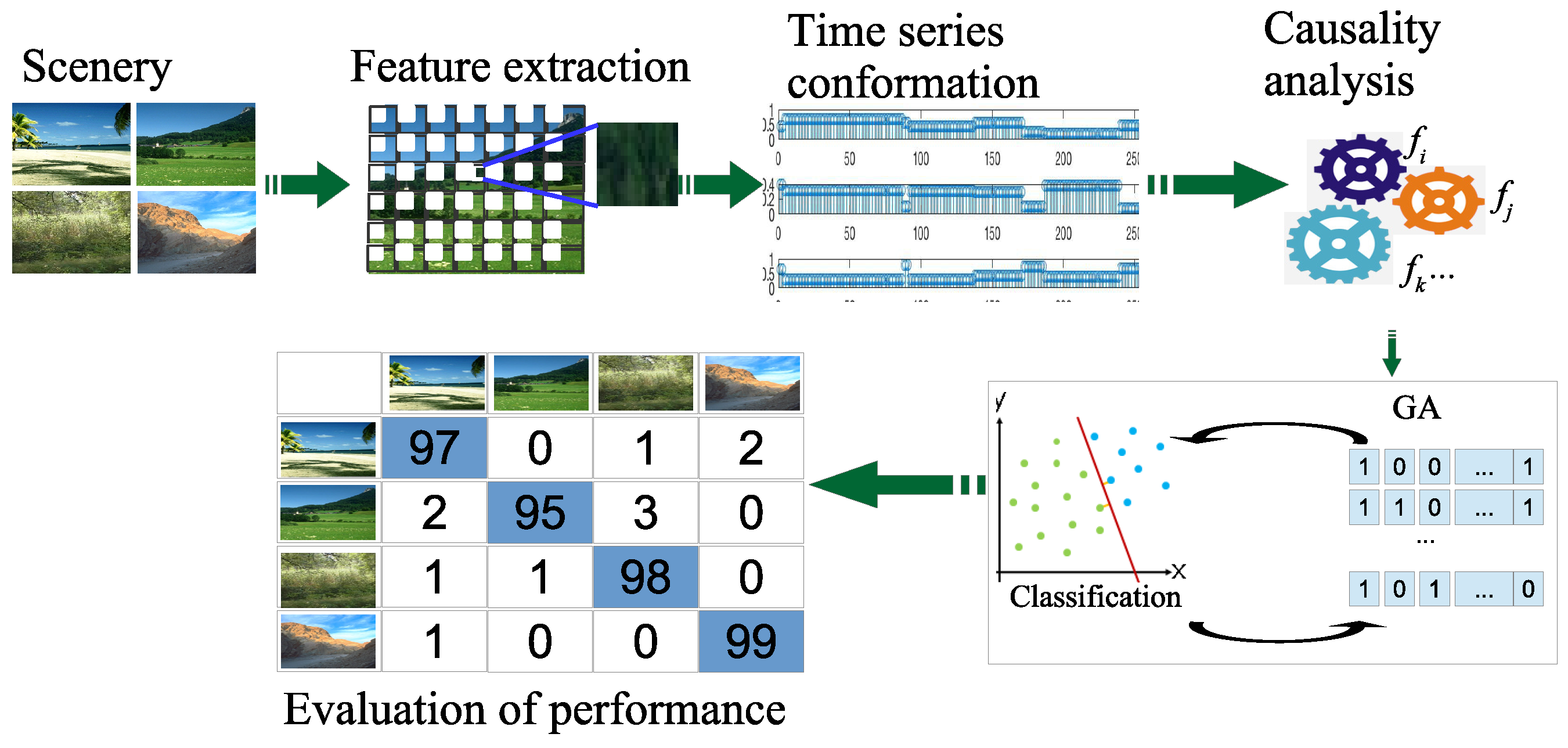
The major stages involved in the developed system are the following (See Figure 1):

• Scenery reading: First, images are read from the data set and then a change of space color format is applied from Red-Green-Blue RGB to Hue-Saturation-Intensity HSI.
• Feature extraction: The statistical CBIR feature extraction is generated within a neighborhood in a grid.
• Time series conformation: The texture features are organized as a time series for each image.
• Causality analysis: The WGC analysis is applied to calculate the causal relationship matrix among different textures.
• Genetic Algorithm (GA) implementation: GA is executed to find the characterization of causality relationships that perform better for natural element retrieval of the images that have similar causality texture patterns for a particular scene.

The paper proposes a causality analysis of the natural scenery classes based on a pre-established texture dictionary and the WGC analysis from the CBIR methodology [5,8] in order to provide a whole dataset characterization.

This approach aims to improve the optimization process of evolutionary algorithms. In this case, since the GA [9] shows a simple and fast implementation, it was employed to select the relationships of the local-texture statistical features handled as time series.

Finally, an improvement in the classification accuracy obtained by our proposed strategy is reported, getting 100% on re-substitution and up to 96% for cross-validation methodologies. This approach was implemented using the computer power of a 19-processor cluster and the MPI parallel programming tool.

The current methodology was probed with two databases of natural scenery:

• Vogel and Shiele (V_S) [10], with 700 Images classified as: 144 coast, 103 forest, 179 mountain, 131 prairie, 111 river/lake and 32 sky/cloud.
• Oliva and Torralba (O_T) [11], with 1472 Images classified as: 360 coast, 328 forest, 374 mountain and 410 prairie.

Visualizing the future implementation of an autonomous system of recognition of natural scenes mounted on a car—which will be managed by our proposal as the autonomous system [12,13,14]—recognizing natural scenarios in the navigation of an autonomous car or possibly a drone, with a 100% certainty, this proposed system will be an important element in the safety of autonomous vehicles.

The rest of the paper is organized as follows: Section 2 presents the state of the art of the problem of image analysis from the CBIR criterion and the WGC theory used in our project, as well as the theoretical support of the WGC model to be applied; in Section 3, the proposed methodology for applying the WGC theory in the natural scenery image characterization is presented; in Section 4 our GA implementation approach to optimize the selection of texture causality relationships is explained; the parallel implementation of our proposal to get good efficiency when processing a large number of images is provided in Section 5; finally, the results and conclusions are presented in Section 6 and Section 8, respectively.

2. State of The Art

The problem of image classification and recognition has been studied with different approaches for supporting visual search for different purposes.

Several techniques have been applied successfully to the face recognition problem [6,15,16,17,18]. The solutions are favored by controlling the way in which the images are obtained by determining the amount of light, the orientation, the distance, and so forth, in order to obtain ideal face images. In addition, the points to be identified on a face image are well known. The multiple textures, objects in unknown positions and their different compositions make it quite difficult to recognize and identify natural scenery in an image or group of images.

One of the most recent solutions for the classification of natural scenery is the use of the deep learning technique [19], which consists of a set of neural networks connected with each other in successive layers, where each layer network performs a convolution operation on the information of the previous layer, as we can see in Reference [20]. This methodology has the disadvantage of requiring high-end computational resources (memory and CPU) for the training task, unlike the CBIR technique which can be implemented in systems with few resources.

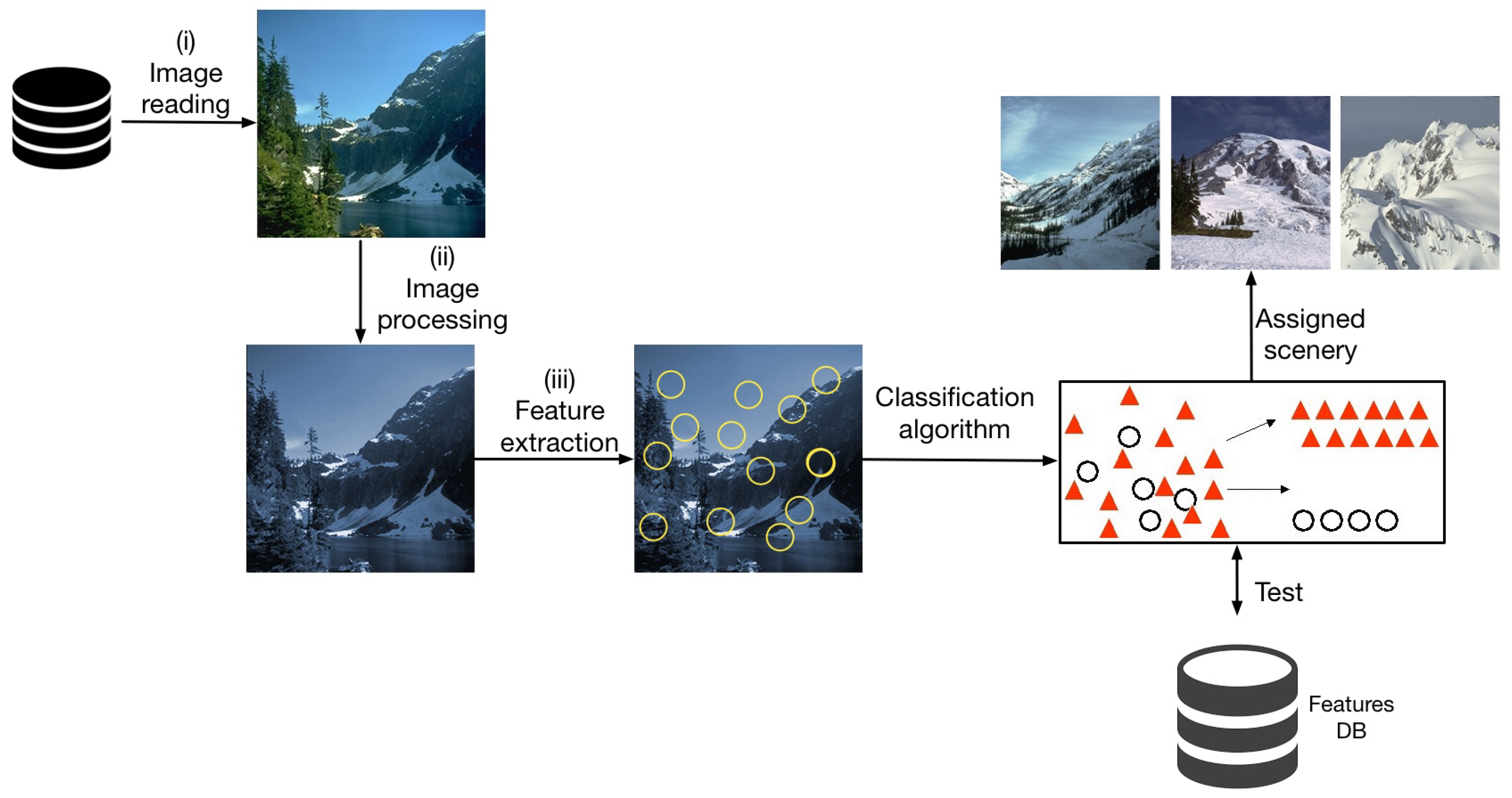
When using CBIR for scenery image classification, significant descriptors are determined considering the image self texture attributes to have an important and effective recovery. In this system, a user presents an image query and the system returns similar images from the database. In Figure 2, the general diagram of a CBIR-based classification system of natural scenery images is shown.

One of the first papers that uses the CBIR methodology for natural scenery classification is that by J. Vogel [21]; this work defines a regular $10\times 10$ grid on the image; from each grid coordinate an analysis window is opened. Local information is extracted from a window texture and compared with a base texture dictionary; then, the author defines a classification system for natural scenery. A point to be improved is the definition of the base texture dictionary that is set manually, including only typical textures perceived by the researchers. This approach obtains up to $75\%$ average for the cross validation classification test.

Unlike a grid, in Reference [8], random points are thrown on the image and around each point a window is opened; from each window, statistical texture local information is extracted to be grouped, conforming dynamically to a base texture dictionary. The testing is performed considering the generated dictionary obtaining an $85\%$ classification average of natural scenery data bases.

In Reference [22], the CBIR approach is presented to classify natural scenery images through the composition of relevant features in relation to the texture, like in Reference [23], the shape and distribution of the luminosity.

CBIR, being an unsupervised learning technique, still has some disadvantages, since the information extracted is only treated as a histogram that represents the composition of textures in a scenery. This way of characterizing scenery has not been able to obtain more than $85\%$ classification, that is why new proposals that use hybrid methodologies to give CBIR greater robustness arise [24]

In References [24,25], the authors combine the CBIR information with certain semantic content introducing high-level concept objects, trying to link content-based images to objects extracted inside them. This work obtained a percentage of natural scenery classification not greater than that of References [21] and [8].

In this work, a hybrid method of three components is presented. The basic component is CBIR, which generates the information regarding the local texture features of the image. Unlike performing only statistical management of the obtained features (using histograms), in this proposal the second component is responsible for applying a causality technique based on the Wiener Granger causality theory to identify the causal relationships that exist within the basic textures of a type of scenery. Since the causality component generates different configurations of causal relationships, the third component consists of a GA that allows the selection of the configuration that obtains the best classification percentage for each scenery.

Evolutionary Computational Vision (ECV) as a research area is currently growing in artificial intelligence through two areas of work—computational vision and evolutionary computation. Beginning from a practical point of view, ECV seeks to design the software and hardware solutions necessary to solve hard computer vision problems [1]. Bio-inspired computation within computational vision contains a set of techniques that are frequently applied to hard optimization problems. Its chief objective is to generate solutions formulated in a synthetic way and the artificial evolutionary process based on the evolutionary theory developed by Charles Darwin is the one frequently applied in Reference [9].

2.1. Theoretical Fundamentals Of Wgc

The causal inference paradigm has been used in different fields of science, for example, in neurology the WGC theory [26] is used to examine areas of the brain and the causal relationships among them. WGC analysis was carried out using sensors [27,28], and, lately in MRI images [29,30,31], the WGC theory is being used for the study of causal relationships among areas of the brain. Other science fields where WGC theory has been applied is video processing for indexing and retrieval [32]. Video processing for massive people and vehicle identification [33,34,35] and complex scenery analysis [36]. In this proposal, for the first time, WGC theory is applied to a natural elements and natural scenes retrieval.

In this section, the theoretical framework of the WGC is established. For simplicity and in order to avoid extending mathematically, the theory is presented only for three random processes, being extendable to $n-$processes. In our approach, a random process corresponds to a signal reading associated to one type of texture within a natural scenery; so, for the present analysis, each texture reading corresponds to one stochastic process represented by $Ti$, being i the i-th texture which has a stochastic behavior disposed into a scenery.

2.2. Stochastic Autoregressive Model

We assume that each texture can be represented by an autoregressive model into time series. In the current analysis, we will only carry out with three signals, {$T1$, $T2$, and $T3$}, being easily extendable to n signals/textures. Let $T1$, $T2$, and $T3$ be three stochastic processes, individually and jointly stationary. Each stationary process can be represented by an autoregressive model in the following way:

$$\begin{array}{cc}\hfill T1\left(t\right)=\sum _{k=1}^{\infty }{C}_{T1}^1\left(k\right)T1(t-k)+{\eta }_{T1}^1,\mathrm{with}& {\sum }_{T1}^1=\mathrm{var}\left({\eta }_{T1}^1\right),\end{array}$$

(1)

$$\begin{array}{cc}\hfill T2\left(t\right)=\sum _{k=1}^{\infty }{C}_{T2}^1\left(k\right)T2(t-k)+{\eta }_{T2}^1,\mathrm{with}& {\sum }_{T2}^1=\mathrm{var}\left({\eta }_{T2}^1\right),\end{array}$$

(2)

$$\begin{array}{cc}\hfill T3\left(t\right)=\sum _{k=1}^{\infty }{C}_{T3}^1\left(k\right)T3(t-k)+{\eta }_{T3}^1,\mathrm{with}& {\sum }_{T3}^1=\mathrm{var}\left({\eta }_{T3}^1\right),\end{array}$$

(3)

being ${\eta }_{T1}^1$, ${\eta }_{T2}^1$ and ${\eta }_{T3}^1$ random Gaussian noise with zero mean and unit standard deviation; $C_{T1}^1\left(k\right)$, $C_{T2}^1\left(k\right)$ and $C_{T3}^1\left(k\right)$ are the coefficients of the regression model for textures $T1$, $T2$ and $T3$, respectively.

The joint autoregressive model for the three textures is defined by the equations:

$$\begin{array}{c}T1\left(t\right)=\sum _{k=1}^{\infty }{C}_{T1}^{1,1}\left(k\right)T1(t-k)+\sum _{k=1}^{\infty }{C}_{T2}^{1,2}\left(k\right)T2(t-k)+\sum _{k=1}^{\infty }{C}_{T3}^{1,3}\left(k\right)T3(t-k)+{\eta }_{T1}^2,\hfill \\ \hfill \mathrm{with}{\sum }_{T1}^2=\mathrm{var}\left({\eta }_{T1}^2\right)\end{array}$$

(4)

$$\begin{array}{c}T2\left(t\right)=\sum _{k=1}^{\infty }{C}_{T1}^{2,1}\left(k\right)T1(t-k)+\sum _{k=1}^{\infty }{C}_{T2}^{2,2}\left(k\right)T2(t-k)+\sum _{k=1}^{\infty }{C}_{T3}^{2,3}\left(k\right)T3(t-k)+{\eta }_{T2}^2,\hfill \\ \hfill \mathrm{with}{\sum }_{T2}^2=\mathrm{var}\left({\eta }_{T2}^2\right)\end{array}$$

(5)

$$\begin{array}{c}T3\left(t\right)=\sum _{k=1}^{\infty }{C}_{T1}^{3,1}\left(k\right)T1(t-k)+\sum _{k=1}^{\infty }{C}_{T2}^{3,2}\left(k\right)T2(t-k)+\sum _{k=1}^{\infty }{C}_{T3}^{3,3}\left(k\right)T3(t-k)+{\eta }_{T3}^2,\hfill \\ \hfill \mathrm{with}{\mathsf{\Sigma }}_{T3}^2=\mathrm{var}\left({\eta }_{T3}^2\right)\end{array}$$

(6)

where ${\mathsf{\Sigma }}_{T1}^2$, ${\mathsf{\Sigma }}_{T2}^2$ and ${\mathsf{\Sigma }}_{T3}^2$ are the variance of the residual terms ${\eta }_{T1}^2$, ${\eta }_{T2}^2$ and ${\eta }_{T3}^2$, respectively. On the other hand, the terms $C_{Tl}^{i,j}\left(k\right)$$\forall i,j,l\in [1,2,3]$, are the regression coefficients for textures $T1\left(t\right)$, $T2\left(t\right)$ and $T3\left(t\right)$, respectively.

Now let us analyze the variances/covariances of the residual terms ${\eta }_{Ti}^2$ by means of the following $\mathsf{\Sigma }$ matrix form Equation (7):

$$\begin{array}{c}\mathsf{\Sigma }=\left(\begin{array}{ccc}{\mathsf{\Sigma }}_{T1}^2& {\mathsf{{\rm Y}}}_{1,2}& {\mathsf{{\rm Y}}}_{1,3}\\ {\mathsf{{\rm Y}}}_{2,1}& {\mathsf{\Sigma }}_{T2}^2& {\mathsf{{\rm Y}}}_{2,3}\\ {\mathsf{{\rm Y}}}_{3,1}& {\mathsf{{\rm Y}}}_{3,2}& {\mathsf{\Sigma }}_{T3}^2\end{array}\right)\hfill \end{array}$$

(7)

where ${\mathsf{{\rm Y}}}_{1,2}$ is the covariance between ${\eta }_{T1}^2$ and ${\eta }_{T2}^2$ (defined as ${\mathsf{{\rm Y}}}_{1,2}=cov({\eta }_{T1}^2,{\eta }_{T2}^2)$); ${\mathsf{{\rm Y}}}_{1,3}$ is the covariance between ${\eta }_{T1}^2$ and ${\eta }_{T3}^2$ (defined as ${\mathsf{{\rm Y}}}_{1,3}=cov({\eta }_{T1}^2,{\eta }_{T3}^2)$), and so on.

Based on the earlier conditions and using the concept of statistical independence between two random processes at the same time (in pairs), causality can be defined in time. An example of the causality between $T1$ and $T2$ is as in the following expression:

$$F_{T2,T1}=ln\left[\frac{{\mathsf{\Sigma }}_{T1}^1\times {\mathsf{\Sigma }}_{T2}^1}{{\mathsf{\Sigma }}_{T{1}^2\times {\mathsf{\Sigma }}_{T2}^2}}\right]$$

(8)

The Equation (8) is commonly known as the causality in the time domain. From this equation, if the random processes $T1\left(t\right)$ and $T2\left(t\right)$ are statistically independent, then $F_{T1,T2}=0$; otherwise there will be causality from one to another.

In the Equation (1), ${\mathsf{\Sigma }}_{T1}^1$ measures the precision of the autoregressive model to predict $T1\left(t\right)$, established on the past samples.

Then again, ${\mathsf{\Sigma }}_{T1}^2$ in the expression (4) measures the precision to predict $T1\left(t\right)$ based on the previous values of $T1\left(t\right)$, $T2\left(t\right)$ and $T3\left(t\right)$ at the same time. Returning to the case of taking only 2 textures at the same time $T1\left(t\right)$ and $T2\left(t\right)$ and according to References [37] and [7], if ${\mathsf{\Sigma }}_{T2}^2<{\mathsf{\Sigma }}_{T1}^1$ then it is said that $T2\left(t\right)$ has a causal influence on $T1\left(t\right)$. The causality is defined by the following equation:

$$F_{T2\to T1}=ln\left[\frac{{\mathsf{\Sigma }}_{T1}^1}{{\mathsf{\Sigma }}_{T1}^2}\right]$$

(9)

It is relatively easy to see that if $F_{T2\to T1}=0$ then there is no causal influence from $T2\left(t\right)$ towards $T1\left(t\right)$, at any other values, the result will be otherwise. On the other hand, the causal influence of $T1\left(t\right)$ towards $T2\left(t\right)$ is established using the following equation:

$$F_{T1\to T2}=ln\left[\frac{{\mathsf{\Sigma }}_{T2}^1}{{\mathsf{\Sigma }}_{T2}^2}\right]$$

(10)

3. Methodology

In the current section, we describe the methodology developed for the WGC technique with a GA support applied to natural scenery.

For the use of the CBIR, there are different determining factors that must be taken into account while extracting the information from the images, such as luminosity, orientation, scale, homogeneity, and so forth. The main characteristic in our proposed patterns is texture, such that we try to create a base dictionary to later create the time series from the reading of the images and their comparison with the dictionary, with which the theory of WGC was applied.

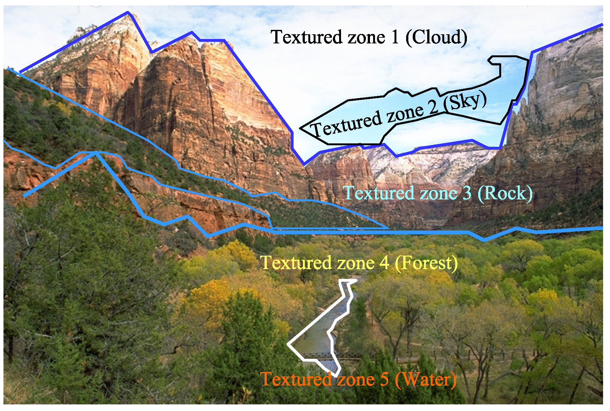
For the development of the dictionary, a set of k textures are manually selected on the images to be studied, which we will call reference textures. The k generated textures represent parts of objects such as the sky, clouds, grass, rock, and so forth, trying to make a manual segmentation of the scenery as shown in Figure 3. In Section 6, the $k=4$ textures test is shown for 6 scenery-classes.

Once the set of the k reference textures has been obtained, the values in the HSI color space of each of them are examined to create a range of maximum and minimum values which represent them, these values help us to define the thresholds of comparison for the test textures of a query image.

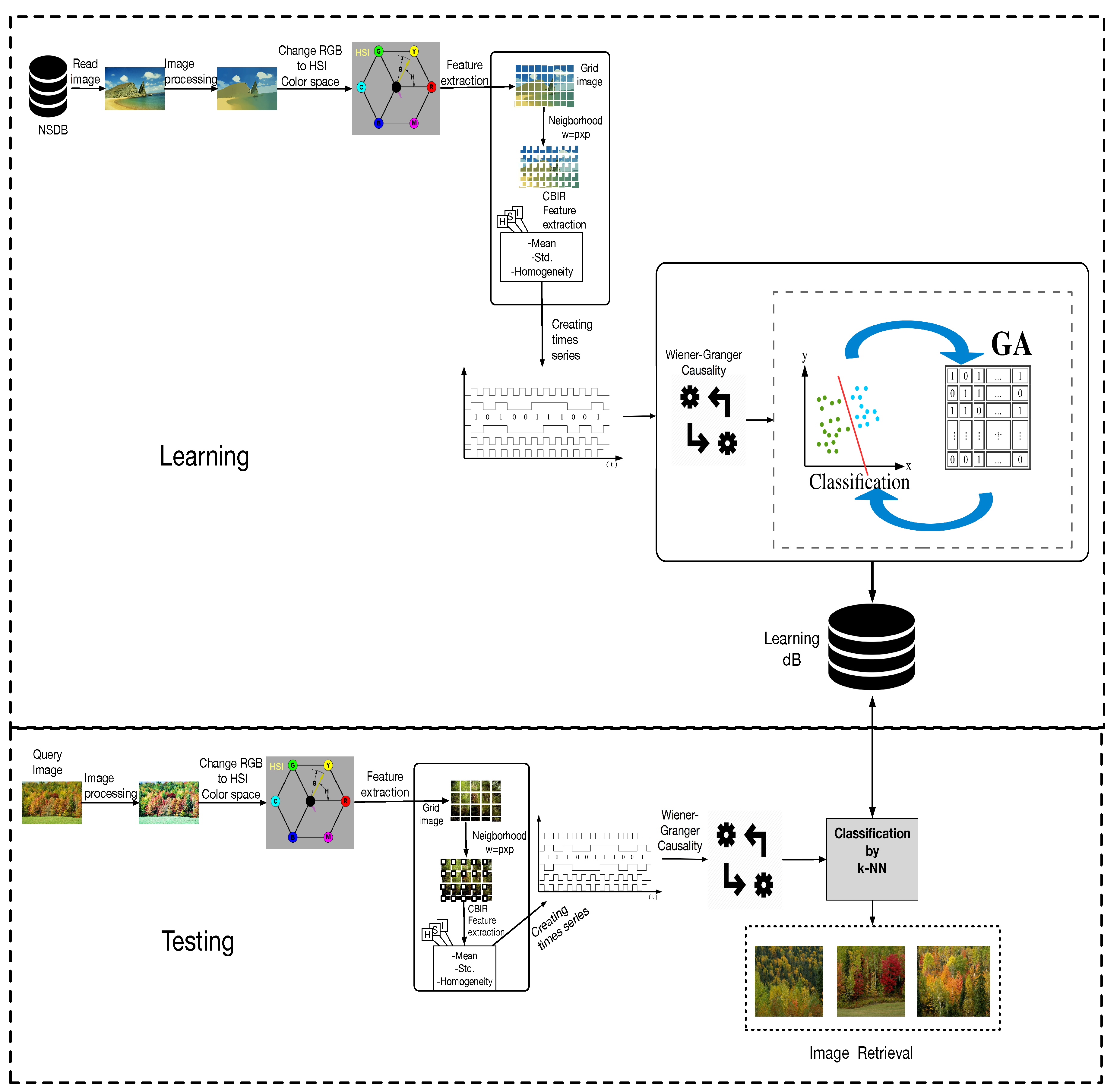
The proposed methodology for the identification and classification of scenery by WGC is shown in Figure 4. The blocks of the architecture are described below.

• Natural Scenery Database (NSDB). Represents the set of images to be analyzed, it contains the images of the natural scenery.
• Reading the images. Is responsible for obtaining the images from the database, which will be processed in (Red-Green-Blue) RGB color format.
• Pre-processing. Pre-processing of the images, erasing the noise, to be used in the next step.
• Change to the (Hue-Saturation-Intensity) HSI color space. The RGB color space does not give us the necessary information for the feature extraction, therefore we pass them/it to the HSI color space, which gives us the information related to the texture.
• Feature extraction. This block consists of three important stages:
  • Grid image. The work done in Reference [21] is taken as a reference, a regular grid of $10\times 10$ windows is considered for the CBIR texture analysis; in our proposal, we use a grid of $r\times c$ windows, which has the property of $r\ne c$, where $c:=$number of windows in horizontal (columns), and $r:=$number of windows in vertical (lines).
  • Neighborhood construction. In each of the resulting frames of the grid, the size of the neighborhood $p\times p$ pixels is extracted, starting from the top left corner of each window, as shown in Figure 5, such that $p<r$ and $p<c$.
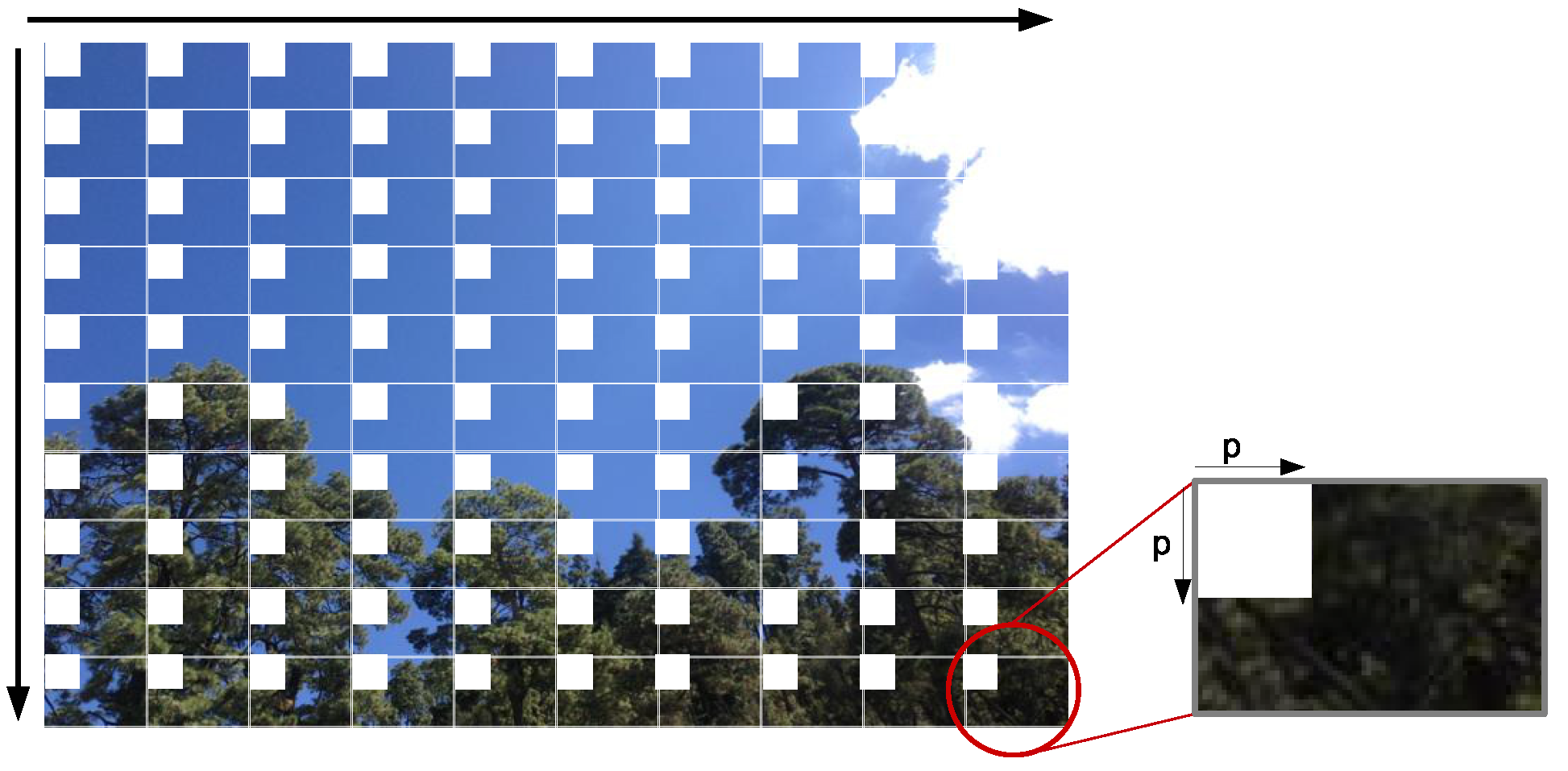
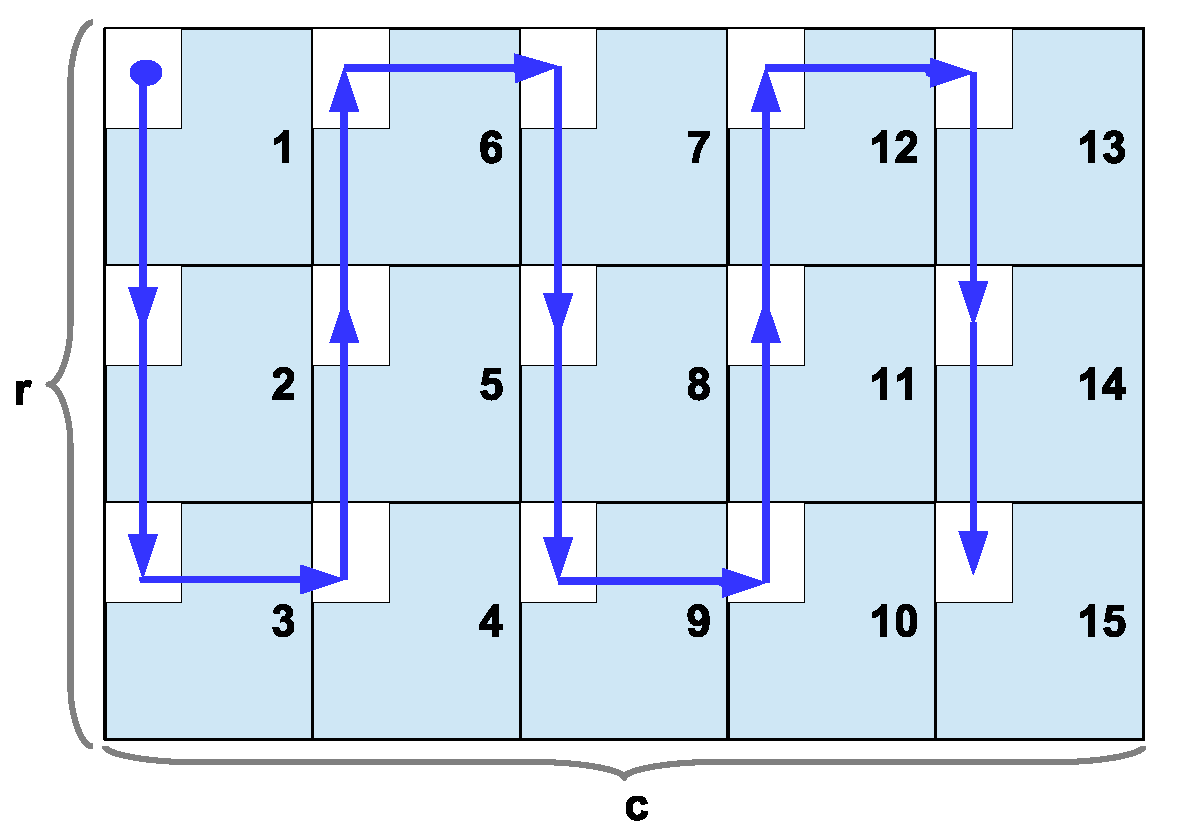
  • CBIR feature extraction. The image is read from the neighborhoods in the following way: It starts in the top left corner of the image and it moves following a descending vertical order through the neighborhoods, processing each of them. Once it reaches the last line, it moves one step to the right neighborhood and goes up to the first line; when the first line is attended again, it moves to the right column within the neighborhood and goes down again (like a snake moving), this reading is repeated for the entire image until the last neighborhood is reached, as shown in Figure 6. Each neighborhood section creates a pattern of size $1\times 3$, that is, one feature per channel (HSI) of the image. After the feature extraction of all the neighborhoods was read in the established order, a matrix $M_s^i$ with size $w\times 3$ is created, where $w=r\ast c$ is the number of neighborhoods analyzed for each i-th image of the class $C_s$.
• Generation of time series.For each $M_s^i$ of the previous step, each matrix entry is compared to the $k-$textures of the dictionary to construct a discrete signal as a time series $T_S^i$, defined as a matrix of size $k\times w$.
  In comparison, the value 1 is assigned if the feature neighborhood approaches the dictionary texture and 0 if not, according to the threshold values which characterize each texture as they were previously presented. After processing the entries of all $M_s^i$, the set of signals for each scenery is stored in the $F{M}_s$, the time series matrix corresponding to a class s that contains $Im{g}_s$ images.
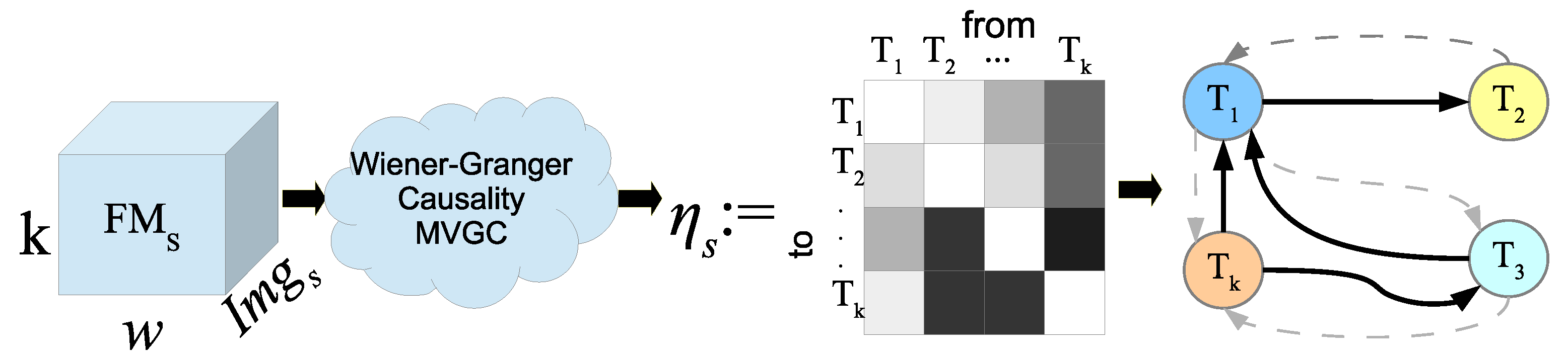
• Wiener-Granger Causality analysis. Each $F{M}_s$ matrix created in the previous step was carried to the WGC analysis to obtain the causal relationships, contained among each one of the base textures. A matrix of causality relationships, ${\mathsf{\eta }}_s$, related to the training images was generated, as shown in Figure 7; therein, darker colors represent stronger relationships and these can be depicted through a state diagram where continuous lines represent only the stronger ones. The analysis of causality was computed with the causality toolbox MVGC [38], which was invoked as an external system call.
  Once the causality analysis has been made for each of the $Cs$ scenery, we get a causality relationships matrix ${\mathsf{\eta }}_s$ of size $k\times k$, with the total of the causal relationships $F_{T_i,T_j}$ from the texture $T_i\to T_j$ (as given in Equation (11)), such that if a value of $F_{T_i,T_j}=0$ means that there is no causal relationship of the texture $i\to j$, and in the measure that the value increases with respect to other ${\mathsf{\eta }}_s$ values, we say that the causal relationship is significant with respect to others.

  $${\mathsf{\eta }}_s=\left[\begin{array}{cccc}{F}_{T_1,T_1}& F_{T_1,T_2}& \cdots & F_{T_1,T_k}\\ F_{T_2,T_1}& F_{T_2,T_2}& \cdots & F_{T_2,T_k}\\ ⋮& ⋮& ⋮& ⋮\\ F_{T_k,T_1}& F_{T_k,T_2}& \cdots & F_{T_k,T_k}\end{array}\right]$$

  (11)

  The causality matrices ${\mathsf{\eta }}_s$ are normalized according to the total sum of their values, being $N_s={\sum }_{i,j=1}^k{F}_{Ti,Tj}$, such that ${\mathsf{\eta }}_s^N$ is the normalized matrix of the $s-$th scenario, for $s=1,\dots ,C_s$, with $C_s$: the number of scenery types considered, as given in the Equation (12). From this resulting matrix the values of the main diagonal are not taken into account because these values do not generate force in the causality relationship; as observed in the theory, there is no causal relationship between the same variables.
  At the end, for $C_s$ classes or scenery, the total concentration of the matrices, $\mathsf{\Gamma }$, is defined as given in the Equation (13).

  $${\mathsf{\eta }}_s^N=\left[\begin{array}{cccc}{F}_{T_1,T_1}& F_{T_1,T_2}& \cdots & F_{T_1,T_k}\\ F_{T_2,T_1}& F_{T_2,T_2}& \cdots & F_{T_2,T_k}\\ ⋮& ⋮& ⋮& ⋮\\ F_{T_k,T_1}& F_{T_k,T_2}& \cdots & F_{T_k,T_k}\end{array}\right]\ast \frac{1}{N_s}$$

  (12)

  $$\mathsf{\Gamma }={\cup }_{l=1}^{Cs}{\mathsf{\eta }}_l^N=\{{\mathsf{\eta }}_1^N,{\mathsf{\eta }}_2^N\cdots {\mathsf{\eta }}_{Cs}^N\}$$

  (13)

  The $\mathsf{\Gamma }$ matrices as entries serve as a descriptive pattern for each scenery or class contained in the database.
• Selection of causal relationships by means of Genetic Algorithm. To look for the causal relationships among different variables that are more important or relevant, for each of the scenes, this can be accomplished in a simple way by eliminating the relationships that have a numerical value less than a previously established threshold.
  However, one disadvantage of this method is the establishment of the threshold to be used, because there is no a priori knowledge of the optimal value; in addition, the complexity increases when the number of textures increases in the dictionary, along with the number of classes and images to be examined. Other drawback of this solution is that some of the weak relationships could also be important in order to characterize a scenery. So there is a need to implement an automatic selection which discriminates the relevant relationships as a combinatorial optimization process. Genetic algorithms (GA) have been used successfully in several computer vision problems together with the digital image processing [39] and classification [1,9,40,41,42]. In this work the GA is also the right solution for the required optimization.

4. Genetic Algorithm Proposal

Looking for the analysis of the $\mathsf{\Gamma }$ matrices generated by the WGC to find the significant causality relationships for one scenery, we propose each matrix to be treated with a GA implementation. In this section we provide the GA proposal in detail.

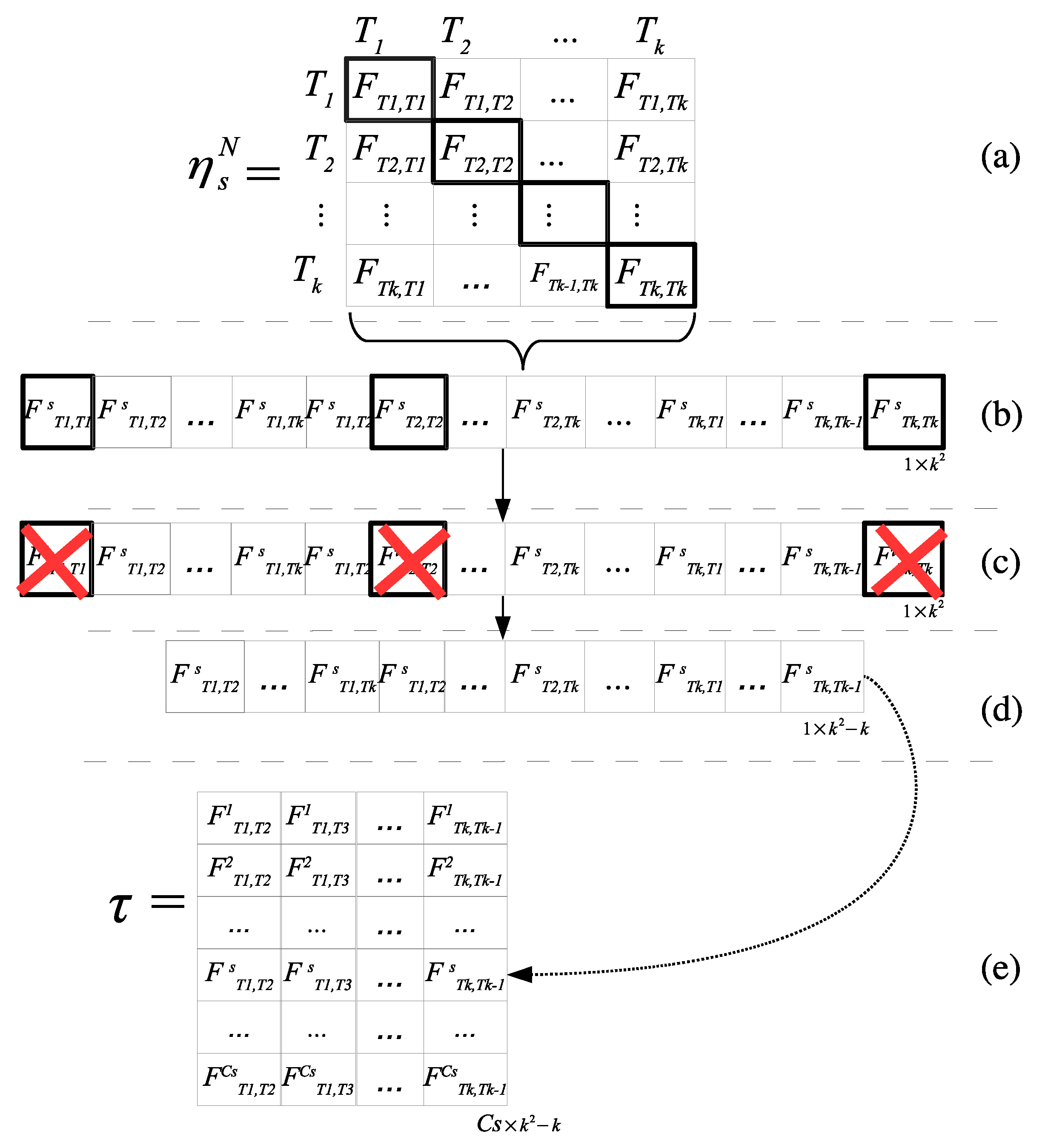
In this approach, each matrix ${\mathsf{\eta }}_s^N\in \mathsf{\Gamma }$ is expressed using vector representation, see Figure 8 parts (a) and (b); this is achieved only by concatenating the rows of the matrix ${\mathsf{\eta }}_s^N$, then the entries of the diagonals are eliminated as shown in Figure 8 part (c). In Figure 8, part (d), a reallocation of the values after the previous elimination is adjusted. This provides a vector of continuous index having the size of each vector $1\times (k^2-k)$ for each $s-$th row, one per scenery. Following this process, finally, the matrix $\mathsf{\tau }$ is created, which contains the linear conformation of each matrix ${\mathsf{\eta }}_s^N$, with $s=\{1,2,\cdots ,Cs\}$ in different rows, as shown in Figure 8 part (e).

4.1. Individual Codification

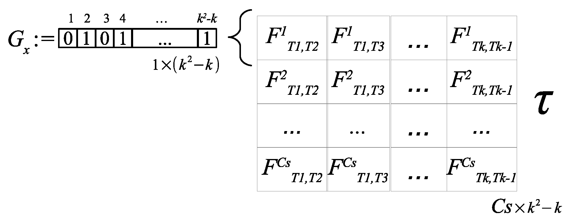
An individual binary representation for one scenery, $\tau \left[i\right]$, is conformed in order to create a filter type array of size $1\times (k^2-k)$ of zeros and ones, such that if an input or causal relationship is selected in that array, the value 1 is used, and 0 if not. So we have $Cs$ rows, one row per scenery, it is intended that each row of the filter matrix could be different from the other lines, with the purpose of characterizing each type of scenery in a unique way.

It is then necessary to apply an automatic process to determine which values of the matrix $\mathsf{\tau }$ are relevant features to distinguish the causal relationships of each scenery, and based on this result, it selects which values are going to be removed for the preset number of textures. With the selection of the most relevant causal values, it is sought to have a classification by means of a distance classifier, towards the matrix $\mathsf{\tau }$ for each one of the query images.

4.2. Fitness Function

The fitness evaluation of each individual is generated in several parts. First, the Equation (14) is applied to the individual $G_x$, representing a texture relationships selection for the $s-$scenery in question, using the matrix $\mathsf{\tau }$ in Figure 9.

$${\rho }_s^{G_x}=\frac{{\displaystyle \prod _{l=1}^{k^2-k}}{G}_x\left(l\right)\ast {\mathsf{\tau }}_{s,l}}{{\displaystyle \sum _{m=1}^{Cs}}{\displaystyle \prod _{l=1}^{k^2-k}}{G}_x\left(l\right)\ast {\mathsf{\tau }}_{m,l}},\mathrm{such}\mathrm{that}{G}_x\left(l\right)\ne 0$$

(14)

There, $\prod G_x\left(l\right)\ast {\mathsf{\tau }}_{s,l}$ refers to the product of the $\mathsf{\tau }$ entries located at $s-$scenery (row s) and column l, specifying a causal relationship, accomplishing $G_x\left(l\right)$ is a valid non zero entry of the genome. Thus ${\rho }_s^{G_x}$ is the total probability for the individual $G_x$ applied to all scenery.

Based on these data, by means of the probability theory, the individual $G_x$ is required to meet the condition: ${\rho }_s^{G_x}>{\rho }_j^{G_x}$, such that $s\in \{1,2,\cdots ,Cs\}$, $s\ne j$, and $1\le j\le Cs$.

That is, $Cs$ probabilities corresponding to each scenery evaluating the individual $G_x$ are obtained with the calculation of ${\rho }_j^{G_x}$. Equation (15) gives the first step for the optimization process, considering the maximum probability related to the casual relationships which best characterized the $s-$scenery versus the others.

$$\underset{s}{\overset{G_x}{\bigvee }}=\left\{\begin{array}{ccc}{\rho }_s^{G_x}& \mathrm{if}& {\rho }_s^{G_x}=Max{\left\{{\rho }_j^{G_x}\right\}}_{j=1,\dots ,Cs}\\ 0& \mathrm{if}& {\rho }_s^{G_x}\ne Max{\left\{{\rho }_j^{G_x}\right\}}_{j=1,\dots ,Cs}\end{array}\right.$$

(15)

Then, the fitness function, $f_s\left(G_x\right)$, is determined as Equation (16).

$$f_s\left(G_x\right)=\left\{\begin{array}{ccc}C{P}_s& \mathrm{if}& {\displaystyle \underset{s}{\overset{Gx}{\bigvee }}}>0\\ 0& \mathrm{if}& {\displaystyle \underset{s}{\overset{Gx}{\bigvee }}}=0\end{array}\right.$$

(16)

To this end, the images contained in the $s-$scenery are consulted, using the re-substitution test. Each image query gives the scenery which belongs to filling the information of a confusion matrix that is used to calculate the percentage of classification. The image consult query process is described in the following paragraph. Later, in Section 4.3 the global fitness is taken into account for the population evolution in the GA loop process.

4.2.1. Creating a Query from a Single Image

In order to classify an s-scenery image considering the relationships specified in a $G_x$ individual, a related causal relationship matrix needs to be constructed.

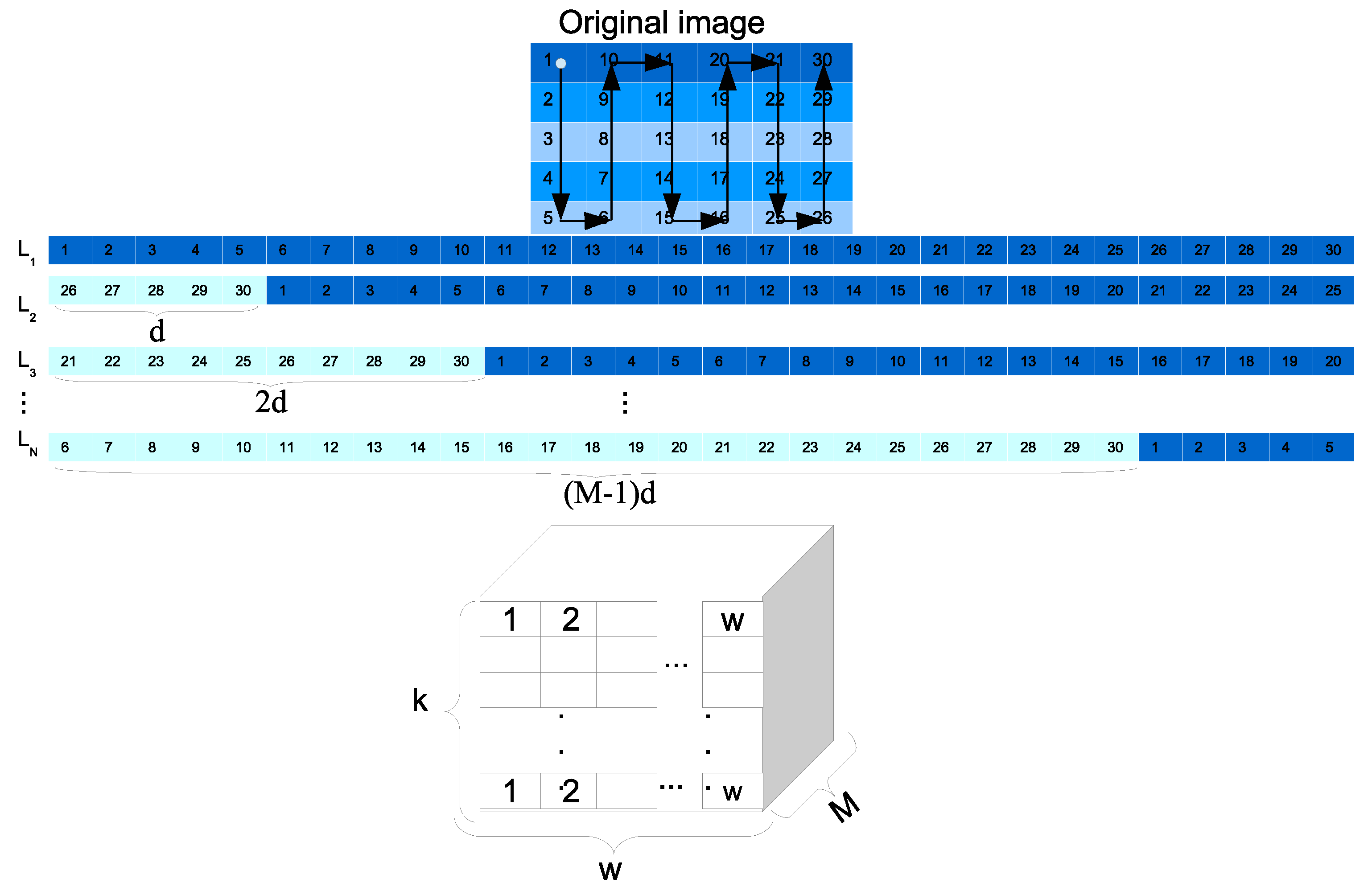
The first step consists of creating a set of M synthetic images, $L_1,L_2,\cdots ,L_M$, from a single L image is performed. This is produced by means of manipulating the first reading of the image, making a circular shift of d positions for each new synthetic image, in order to create several samples of the same image as shown in Figure 10. In this way, the respective query matrix of size $|k\times w\times M|$ ($k:=$ number of textures in the dictionary, $w:=$ number of neighborhoods, and $M:=$ number of synthetic images) is generated to feed the WGC analysis process and to obtain the resulting normalized causal relationship matrix ${\mathsf{\eta }}_L^N$ of size $|k\times k|$. These steps are carried out by Equations (11) and (12).

Then the manipulation of ${\mathsf{\eta }}_L^N$ is performed as shown in the stage presented in Figure 8 to obtain the linear representation of the matrix. The last query step consists of applying the k-NN classifier (with $k:=1$) to determine which $\mathsf{\tau }$ scenery (line) has the closest relationship to the linear relationship representation of image L, considering only the relationship indicated with the $G_x$ non-zero values.

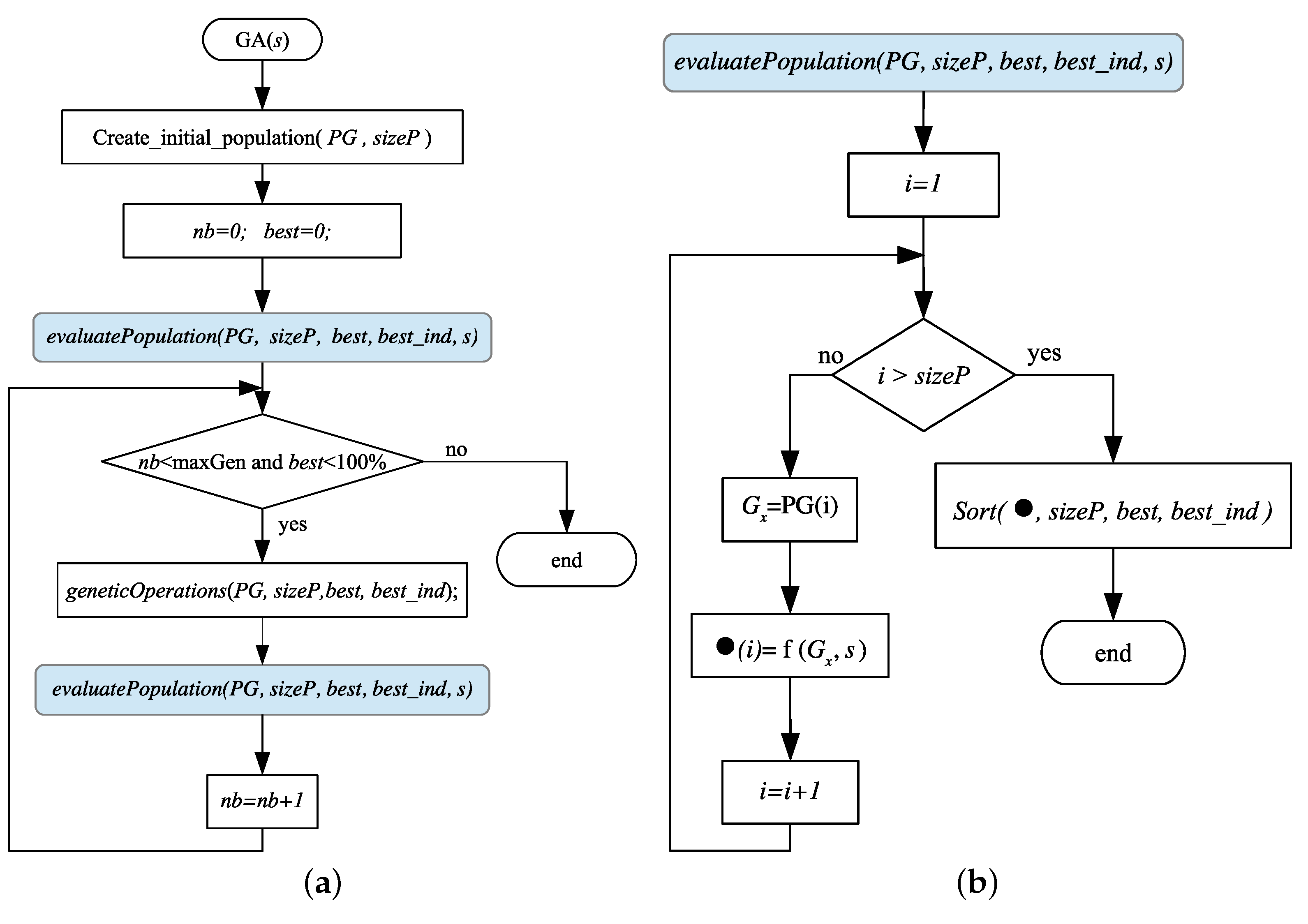
4.3. GA Implementation

A genetic algorithm is applied for each $\mathsf{\tau }$ line to automatically select the most representative causal relationship of each scenery. Figure 11a shows the general algorithm flowchart of this approach.

An initial population, $PG$, of $sizeP$ individuals is randomly generated, where $sizeP$ is an odd number and each individual is of size $k^2-k$, the size in columns of the matrix $\mathsf{\tau }$.

Then the $PG$ individuals are evaluated with the fitness function, Equation (16), for a particular $s-$scenery, considering the total set of images that conform it, as shown in Figure 11b. The individual’s fitness is stored inside a fitness array $\{•\}$, as in Equation (17). The $\{•\}$ array is consequently ordered, from highest to lowest, to find the best individual with the highest fitness.

$$\{•\}=\{f_1\left(G_x\right),f_2\left(G_x\right),\dots ,f_{sizeP}\left(G_x\right)\},$$

(17)

such that $f_p\left(G_x\right)\ge 0$ for $1\le p\le sizeP$. For this proposal, size population $sizeP=21$, the genome length is 12, and the number of iterations was $maxGen=100$ generations.

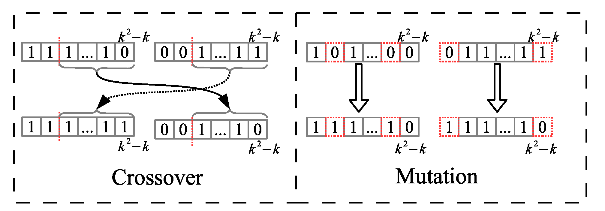
To generate the new population, $\left(sizeP-1\right)/\phantom{\left(sizeP-1\right)2}2$ triplets of random numbers are generated, e.g., {1,5,1} or {2,4,0}, where the first two numbers are the selected individual numbers that generate the new individuals, the third element of the triplet is one of the two possible operations to be executed; either crossover “1” or mutation “0”.

For derivatives of each triplet, we generate two new individuals if it is by crossover operator, or if it is by mutation operator the two selected individuals are altered separately, in order to have two new elements for the new generation, 1 mutated individual from one single individual.

The crossover operator is applied at one uniform random point of the two participating chromosomes, and the mutation operator is performed over $10\%$ of the elements of a chromosome, as shown in Figure 12.

The genetic operations of mutation and crossover are applied to $30\%$ and $70\%$ of the population respectively, favoring the selection of the highest fitness individuals to be reproduced. The individual with the best fitness passes to the next generation applying elitism. In this way, the population will evolve towards a selection of relevant causal relationships to be able to characterize each scenery.

The end of the GA or stop criteria is given when reaching the $100\%$ classification percentage or a number of generations is attained.

After the GA is applied $Cs$ times, the individuals that contain the most relevant relationships for each scenery are found. Then, the $\mathsf{\tau }$ matrix is updated and its entries are replaced by a zero value whenever the corresponding individual entries have a zero and they keep their value in other case.

5. Parallel Approach

In this section, a parallel algorithm to speed-up the performance of the proposed WGC methodology is presented. The parallel approach works on a distributed memory architecture using MPI library; that is, there is a set of processes without shared memory, and these processes work in parallel, and the communication goes through message exchange to determine the relevant causal relationships of all the scenery. Each process can access the NSDB to extract and work with the corresponding set of images. The algorithm complexity in this proposal is given for the Equation (18).

$$O(N_{class}\times k\times CIP\times r\times c\times nImg\times t_{comp}\times WG{C}_{tb})$$

(18)

where, $N_{class}:=$ number of classes, $k:=$ number of textures, $CIP:=$ constant for every image processing, $r:=$ number of rows in the grid, $c:=$ number of cols in the grid, $nImg:=$ total number of images, $t_{comp}:=$ comparison time against the base textures, $WG{C}_{tb}:=$ causality analysis time. (e.g., for an image of size $640x480$ pixels, $r=(640/20)$, $c=(480/30)$, and p is the size of the neighborhood, such that $10\times 10$ implies $p=10$) That means, if the number of rows r, cols c in the grid increases, then the number of images nImag in NSDB increases, and the number of base textures k in the dictionary increases, and the number of classes $N_{class}$ increases, thus the computational cost increases. In this way it is necessary to conceive a parallel architecture to solve this problem in a large number of images related to Big Data problems.

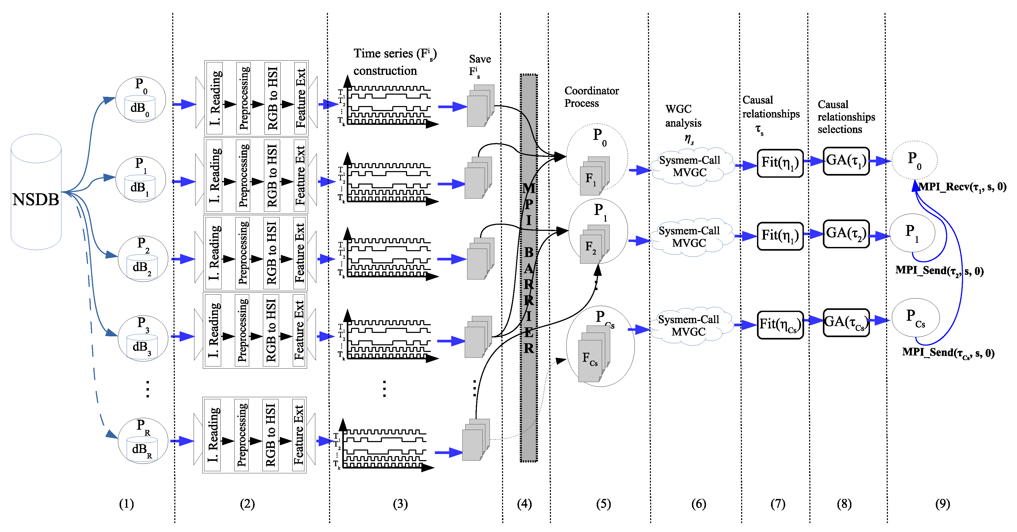
The Algorithm 1 shows the procedure which is executed simultaneously by each process and the general process of this parallel proposal is depicted in Figure 13.

At the beginning (line 2 of Algorithm 1, Figure 13, tag (1)), each process determines the amount set of images to be read (ImgBlock), taking into consideration the total number of images ($Total\_IMGs$), the total number of processes ($Total\_procs$) and the process identifier (rank). A single process can work with images belonging to different scenery (e.g., $Total\_IMGs=700$, $Total\_procs=70$, $imgBlock=700/10=10$ for the $NSDB$).

Algorithm 1 Parallel algorithm for the causality matrix construction.

1: procedureCausality matrix construction(rank) 2:     initialization(ImgBlock,Total_IMGs,Total_procs,rank); 3:     for every i in ImgBlock do 4:         $Img\_RG{B}_{r}ead(image,s,i)$; 5:         $Img\_preprocessing\left(image\right)$; 6:         $RGB\_to\_HSI\left(image\right)$; 7:         $M_s^i$= Feature_extraction(image); 8:         $F_s^i$= time_series_construction($M_s^i$, $Texture\_Dictionary$); 9:         Save_TimeSeries($F_s^i$); 10:     end for 11:     $Barrier\_synchronization\left(\right);$ 12:     if rank in {Scenery coordinator ranks} then 13:         $F_s$= Load_all_time_series(s); 14:         ${\mathsf{\eta }}_s$= $System\_call\left(MVGC\left(F_s\right)\right);$ 15:         ${\mathsf{\tau }}_s$= Fitting $\left({\mathsf{\eta }}_s\right);$ 16:         Genetic_Algorithm$\left({\mathsf{\tau }}_s\right);$ 17:         Send $({\mathsf{\tau }}_s,s,General\_coordinatorrank);$ 18:     end if 19:     if (rank == $General\_coordinatorrank$) then 20:         for (every $id$ in {Scenery coordinator ranks}) do 21:            Recv $({\mathsf{\tau }}_s,s,id);$ 22:            $\mathsf{\tau }\left(s\right)$= ${\mathsf{\tau }}_s;$ 23:         end for 24:     end if 25: end procedure

Each process works simultaneously with the section of the NSDB, $ImgBlock$, which was assigned to it, performing the following steps (lines 3–10). The reading of the i-image in RGB space is the first action to be executed, next up the scenery, s, such that i-image $\in s$, is also obtained (line 4). Then the image preprocessing and the conversion from RGB to HSI domains are carried out (lines 5 and 6, respectively). In line 7, the statistical features are calculated, including the construction of the image grid and neighborhoods, then the CBIR features per each neighborhood generates the $M_s^i$ matrix; Figure 13, tag (2), represents the execution of lines 4 to 7 of Algorithm 1. Then, $M_s^i$ and the texture dictionary are used to construct the respective time series, $F_s^i$, that is stored on file (lines 8,9 of the algorithm, Figure 13, tag (3)).

Up to this point, all processes work independently; however, in order to ensure that every process has fully accomplished its task, a parallel barrier synchronization (line 11 of the algorithm, Figure 13, tag (4)) should be introduced before continuing with the next step. Here (line 12), only the processes identified as $scenerycoordinators$ (one process per scenery) continue with the construction of the corresponding $F_s$ matrix (line 13, Figure 13, tag (5)), by loading the respective set of $F_s^i$ matrices (one per scenery image), previously generated. Then, a system call is performed (line 14, Figure 13, tag (6)) to run the MVGC toolbox and obtain the causality relationship matrix, ${\mathsf{\eta }}_s$, from the WGC analysis.

The $Fit\left({\mathsf{\eta }}_s\right)$ function in line 15 (Figure 13, tag (7)) is in charge of normalization and vector representation of the causality relationship matrix, ${\mathsf{\eta }}_s$. The respective ${\mathsf{\tau }}_s$ is thus generated, corresponding to the s-th row (scenery) of $\mathsf{\tau }$ matrix. Line 16 of Algorithm 1 (Figure 13, tag (8)) shows the GA call that is executed by each one of the $Cs$ scenery coordinator processes, with $Cs$ being the number of scenery. After identifying the most relevant causal relationships by means of the GA, ${\mathsf{\tau }}_s$ is updated and sent to the general coordinator (line 17) through a message.

Finally, in lines 19–24, the general coordinator process receives, by means of several messages, the results generated by the scenery coordinator processes (Figure 13, tag (9)). When all message receptions are achieved, the matrix $\mathsf{\tau }$ is successfully constructed.

6. Experimental Results

The proposal evaluation was generated using the computer power of a 19-processor dual core cluster. Each processor is an Intel©Xeon©CPU E5-2670 v3 2.30 GHz, and 74 GB RAM.

Four image textures $k=4$ where selected to conform the base dictionary, as shown in

Table 1. HSI ranges of the base texture dictionary.

Texture	H-max	H-min	S-max	S-min	I-max	I-min
Cloud	180	0	25	0	255	61
Sky	113	93	255	25	61	255
Rock	24	6	255	20	190	30
Forest	102	28	255	10	229	3

. For each texture the generated values were obtained manually within the images of the database, a set of 20 texture samples were taken from a set of 5 images per class, from each texture the average was extracted in the layer H plus twice the standard deviation, with this the maximum and minimum threshold values for each texture were generated.

The $NSDB$ used for the evaluation consists of the following data:

• Vogel and Shiele (V_S) [10], including 6 scenery with 700 images classified as: 144 coast, 103 forest, 179 mountain, 131 prairie, 111 river/lake, and 32 sky/cloud.
• Oliva and Torralba (O_T) [11], including 4 scenery with 1472 Images classified as: 360 coast, 328 forest, 374 mountain and 410 prairie.

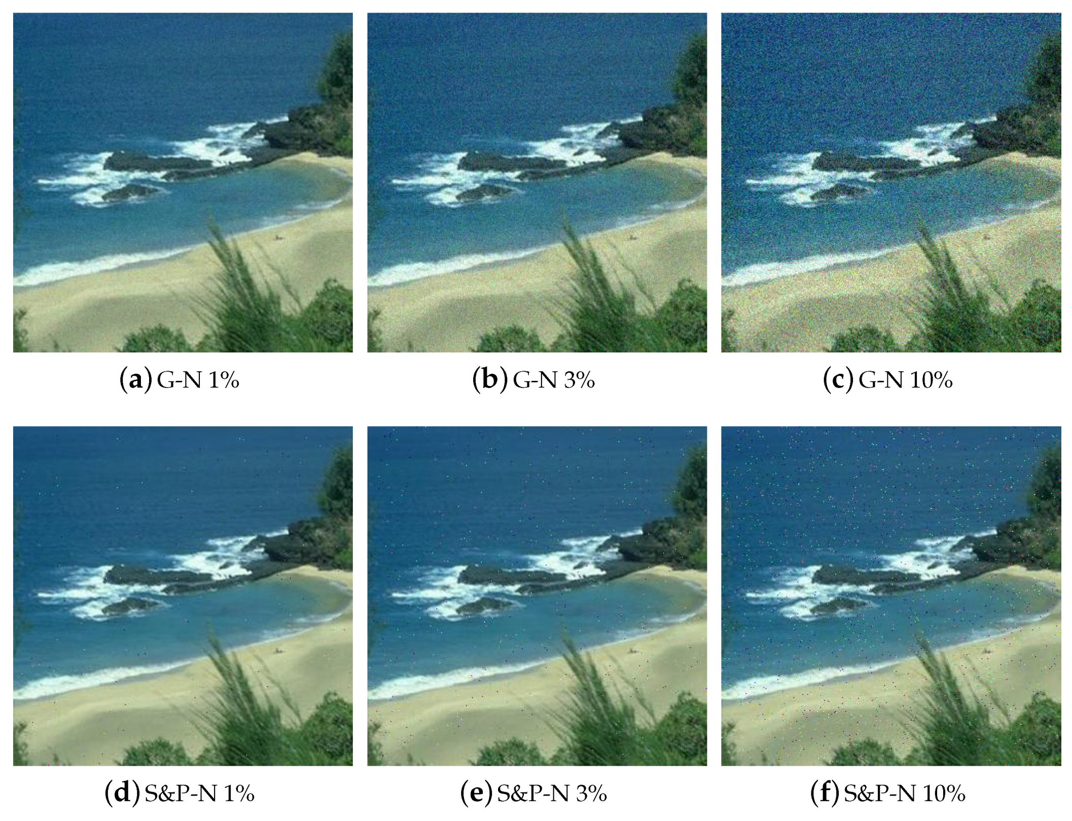
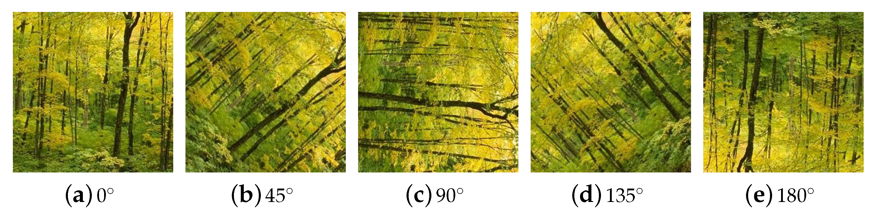
The images were adapted so that some typical classification challenges were considered. The whole set of images was tested in a normal state and introducing Gaussian noise (GN), salt and pepper noise (S&P) of $1\%,3\%$, and $10\%$ levels respectively, as shown in Figure 14. A rotation transformation was also introduced on each image considering $0^{\circ }$, ${45}^{\circ }$, ${90}^{\circ }$, ${135}^{\circ }$, and ${180}^{\circ }$, as shown in Figure 15. An image consult query was performed following the same procedure described in Section 4.2.1.

The results in this section are organized as follows. The image classification performance obtained when applying the WGC theory is first presented. Then the execution times of the proposed parallel methodology are shown.

6.1. Classification Results

To show that the proposed GA implementation was a good solution to select some relevant texture relationships describing a scenery, we compared our proposal (GA version) to the manual strategy (Manual version) introduced in Reference [36]; under the manual strategy only the highest relationship values were selected, establishing a specific threshold. In both versions, the methodology presented in Section 3 for the construction of $\mathsf{\tau }$ matrix, was executed.

Table 2. The obtained $\mathsf{\tau }$ matrix values.

Scene/F	${\mathit{F}}_{\mathit{T}1,\mathit{T}2}$	${\mathit{F}}_{\mathit{T}1,\mathit{T}3}$	${\mathit{F}}_{\mathit{T}1,\mathit{T}4}$	${\mathit{F}}_{\mathit{T}2,\mathit{T}1}$	${\mathit{F}}_{\mathit{T}2,\mathit{T}3}$	${\mathit{F}}_{\mathit{T}2,\mathit{T}4}$	${\mathit{F}}_{\mathit{T}3,\mathit{T}1}$	${\mathit{F}}_{\mathit{T}3,\mathit{T}2}$	${\mathit{F}}_{\mathit{T}3,\mathit{T}4}$	${\mathit{F}}_{\mathit{T}4,\mathit{T}1}$	${\mathit{F}}_{\mathit{T}2,\mathit{T}4}$	${\mathit{F}}_{\mathit{T}3,\mathit{T}4}$
Forest	0.370	0.289	0.0051	0.0269	0.037	0.0013	0.108	0.075	0.0849	0.00332	1.611 $\times {10}^{-5}$	0.00062
Sky & cloud	0.0441	0.0481	0.0321	0.0269	0.343	0.197	0.0044	0.0385	0.211	0.011	0.0070	0.0371
Coast	0.0099	0.233	0.188	0.021	0.0363	0.0503	0.0542	0.0014	0.0646	0.1558	0.0772	0.109
Mountain	0.085	0.405	0.0132	0.0497	0.0799	0.0698	0.1115	0.0102	0.0162	0.1076	0.0392	0.0133
Prader	0.2401	0.1143	0.2400	0.0045	0.0140	0.0268	0.2151	0.1146	0.0006	0.0161	0.0140	0.0002
River	0.1619	0.4053	0.1112	0.0061	0.0046	0.0035	0.0377	0.0322	0.1794	0.0066	0.0084	0.0432

shows the resulting $\mathsf{\tau }$ values.

Because there were no a priori criteria to determine a threshold value, in the Manual version $25\%$ of the less significant causal relationships per scenery were deleted.

Table 3. The $\mathsf{\tau }$ matrix resulting from the manual selection of the highest significant causal relationships.

Scene/F	${\mathit{F}}_{\mathit{T}1,\mathit{T}2}$	${\mathit{F}}_{\mathit{T}1,\mathit{T}3}$	${\mathit{F}}_{\mathit{T}1,\mathit{T}4}$	${\mathit{F}}_{\mathit{T}2,\mathit{T}1}$	${\mathit{F}}_{\mathit{T}2,\mathit{T}3}$	${\mathit{F}}_{\mathit{T}2,\mathit{T}4}$	${\mathit{F}}_{\mathit{T}3,\mathit{T}1}$	${\mathit{F}}_{\mathit{T}3,\mathit{T}2}$	${\mathit{F}}_{\mathit{T}3,\mathit{T}4}$	${\mathit{F}}_{\mathit{T}4,\mathit{T}1}$	${\mathit{F}}_{\mathit{T}2,\mathit{T}4}$	${\mathit{F}}_{\mathit{T}3,\mathit{T}4}$
Forest	0.370	0.289	0.0051	0.0269	0.037	0	0.108	0.075	0.0849	0.00332	0	0
Sky & cloud	0.0441	0.0481	0.0321	0.0269	0.343	0.197	0	0.0385	0.211	0	0	0.0371
Coast	0	0.233	0.188	0	0.0363	0.0503	0.0542	0	0.0646	0.1558	0.0772	0.109
Mountain	0.085	0.405	0	0.0497	0.0799	0.0698	0.1115	0	0	0.1076	0.0392	0
Prader	0.2401	0.1143	0.2400	0	0.0140	0.0268	0.2151	0.1146	0	0.0161	0.0140	0
River	0.1619	0.4053	0.1112	0	0	0	0.0377	0.0322	0.1794	0	0	0.0432

shows the updated $\mathsf{\tau }$ matrix after the manual selection.

When executing the GA version for the selection of $\mathsf{\tau }$ matrix relationships, a larger space of solutions was explored trying to look for the causal relationships that best represent one scenery. The obtained individuals are presented in

Table 4. The best individuals resulting from the evaluation of the GA per scenery.

Scene/F	1	2	3	4	5	6	7	8	9	10	11	12
Forest	1	0	0	0	0	0	0	0	1	0	0	0
Sky	0	1	1	0	1	1	1	1	0	0	0	1
Coast	0	0	1	1	0	0	0	1	0	0	1	1
Mountain	1	0	0	1	0	0	1	1	0	0	0	1
Prader	1	0	1	0	1	0	1	1	1	0	1	0
River	0	0	1	1	0	0	1	1	0	0	0	1

, and the updated $\mathsf{\tau }$ matrix is shown in

Table 5. Final $\mathsf{\tau }$ values, applying the better individuals of the GA.

Scene/F	${\mathit{F}}_{\mathit{T}1,\mathit{T}2}$	${\mathit{F}}_{\mathit{T}1,\mathit{T}3}$	${\mathit{F}}_{\mathit{T}1,\mathit{T}4}$	${\mathit{F}}_{\mathit{T}2,\mathit{T}1}$	${\mathit{F}}_{\mathit{T}2,\mathit{T}3}$	${\mathit{F}}_{\mathit{T}2,\mathit{T}4}$	${\mathit{F}}_{\mathit{T}3,\mathit{T}1}$	${\mathit{F}}_{\mathit{T}3,\mathit{T}2}$	${\mathit{F}}_{\mathit{T}3,\mathit{T}4}$	${\mathit{F}}_{\mathit{T}4,\mathit{T}1}$	${\mathit{F}}_{\mathit{T}2,\mathit{T}4}$	${\mathit{F}}_{\mathit{T}3,\mathit{T}4}$
Forest	0.370	0	0	0	0	0	0	0	0.0849	0	0	0
Sky&cloud	0	0.0481	0.0321	0	0.343	0.197	0.0044	0.0385	0	0	0	0.0371
Coast	0	0	0.188	0.021	0	0	0	0.0014	0	0	0.0772	0.109
Mountain	0.085	0	0	0.0497	0	0	0.1115	0.0102	0	0	0	0.0133
Prader	0.2401	0	0.2400	0	0.0140	0	0.2151	0.1146	0.0006	0	0.0140	0
River	0	0	0.1112	0.0061	0	0	0.0377	0.0322	0	0	0	0.0432

.

Both, GA and manual versions where tested using 300 images, 50 per scenery. The manual version only obtained obtaining a $12.53\%$ general classification percentage. The confusion matrix showing the image association per scenery can be seen in

Table 6. Confusion matrix for a test with 50 images per scenery, using a manual selection of causal relationships.

Scenei/Scenej	Forest	Sky	Coast	Mount	Prad	Riv
Forest	0	0	31	19	0	0
Sky	1	0	39	10	0	0
Coast	3	0	36	11	0	0
Mount	2	0	47	1	0	0
Prad	5	0	40	5	0	0
Riv	6	0	32	11	1	0

; we observe that most of the images were associated to the coast scenery, and as a result the manual selection test gave a poor classification percentage.

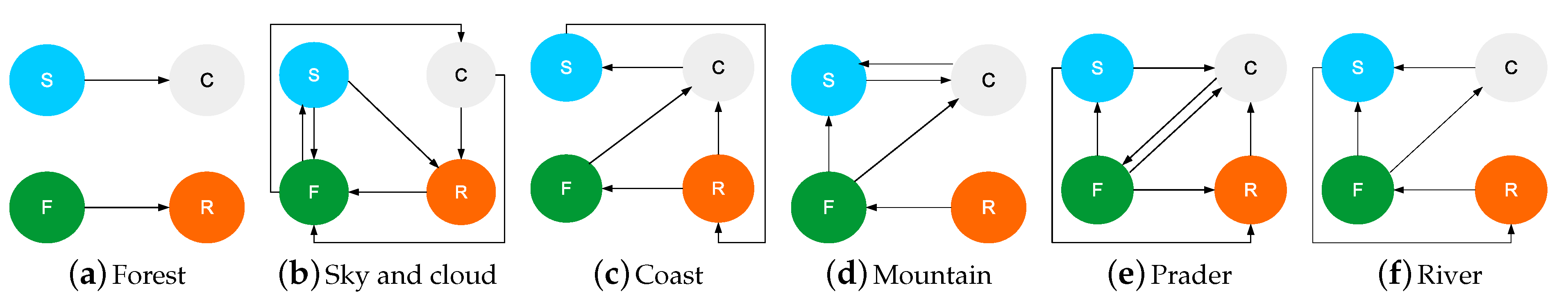
With the information in the Table 5, the most representative relations of each natural scenery are generated as a visual representation, the graphs representing the intensity of the causal relations between the $k=4$ base textures of the dictionary. These graphs will show how textures are related within the corresponding scenery, obtaining the pattern which represents each of them, as it can be appreciated in Figure 16.

Given these first results, it can be observed that not necessarily the relationships with higher values were the best ones to be selected.

To measure the technical efficiency of our proposal using the GA, the Recall (managed as classification percentage), Precision, Accuracy and F1 Score were estimated from the confusion matrices of every test.

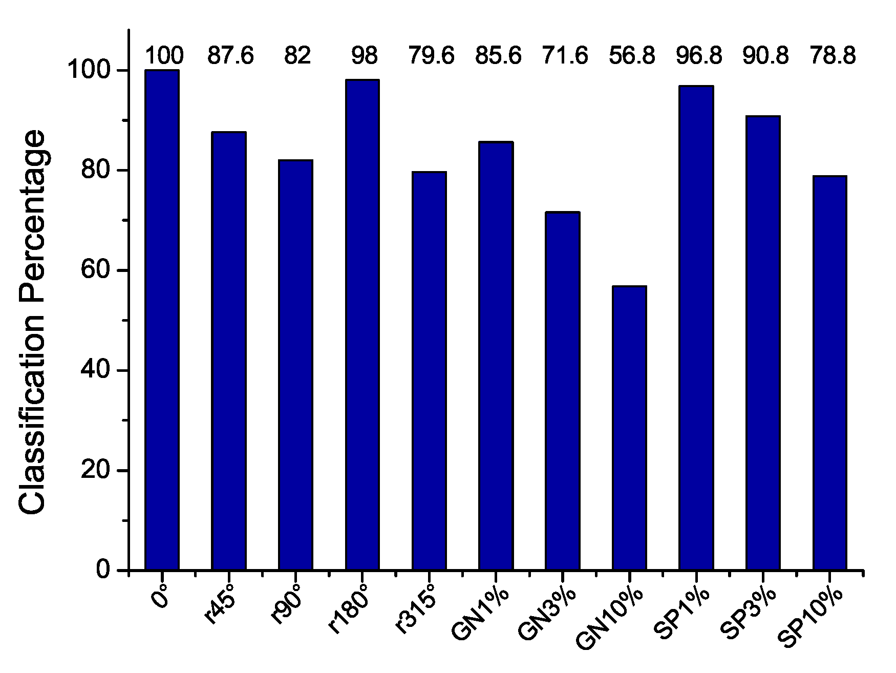
The classification results of Figure 17 show that that rotating the images by ${45}^{\circ }$, ${90}^{\circ }$ and ${315}^{\circ }$, the classification performance decays significantly. Also, the noise (GN and S&P) significantly alters the classification which is expected in natural scenery images since the texture is a representative of the type of image, and the alterations with noise on it degenerate into another possible meaning. In normal conditions, avoiding noise and rotations, the classification performance reaches 100%.

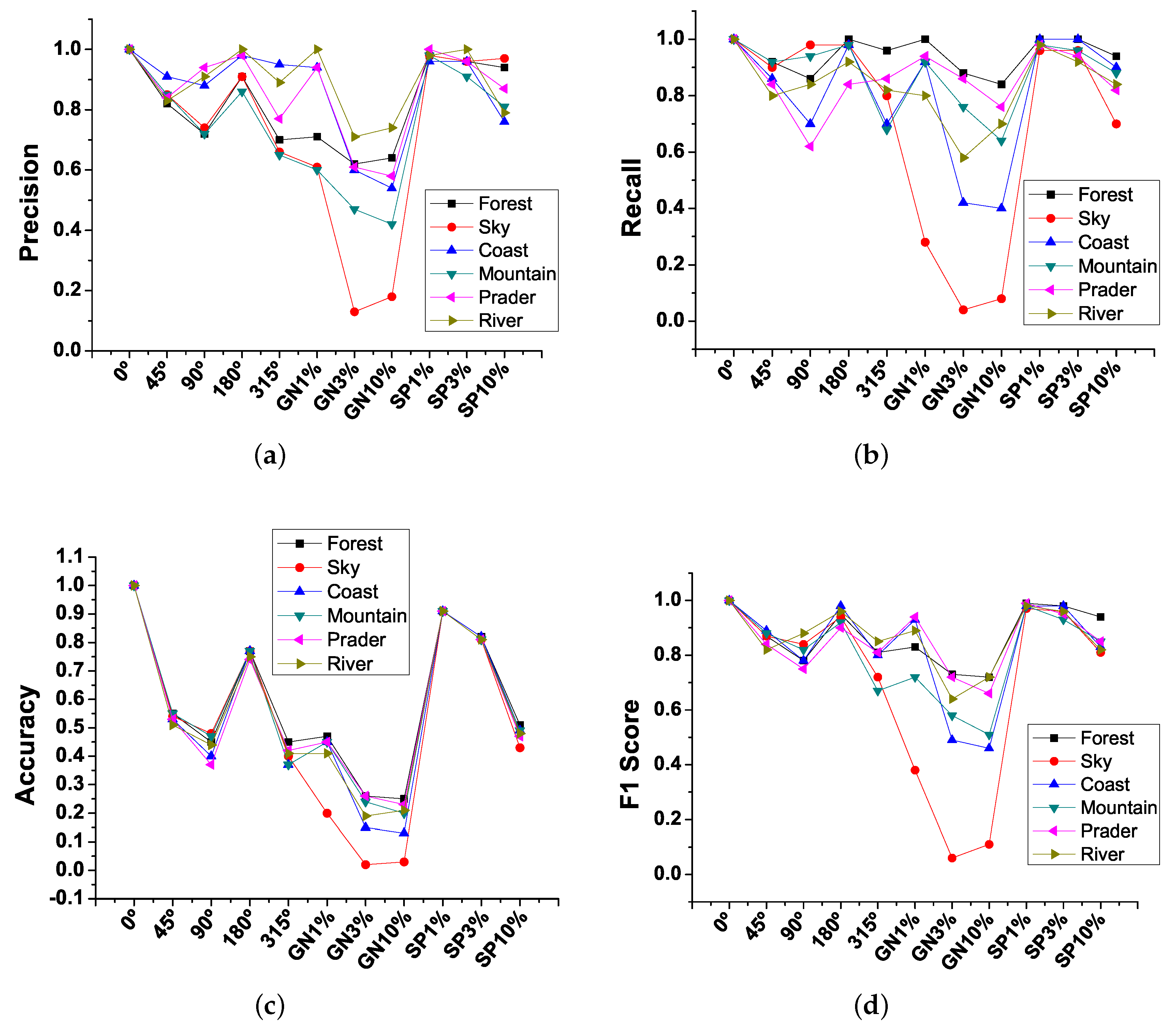
Additionally, Figure 18 shows the estimations of the precision (Figure 18a), recall (Figure 18b), accuracy (Figure 18c), and F1 Score (Figure 18d) averages for the classes contained in the NSDB. In general, the classification of ideal images ($0^{\circ }$) without rotations and noise obtains 100% classification, However, when rotations and noise are added this percentage decreases, particularly the sky class is the most affected.

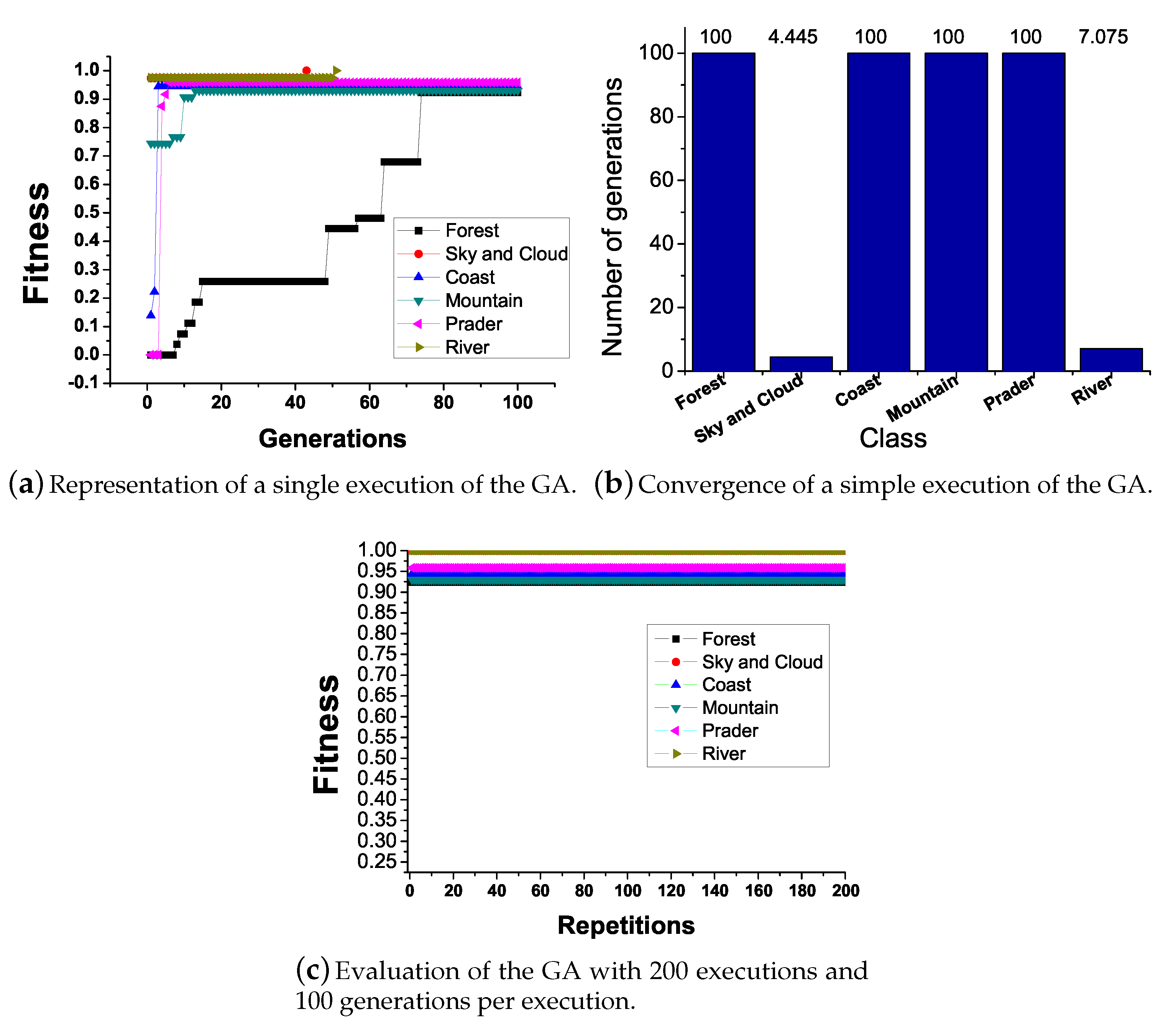
The average result for the GA evaluation is depicted in Figure 19. Figure 19a shows the fitness evolution within a run with 100 generations. Figure 19b shows that, while in some classes the highest fitness is achieved in the first iteration, in the other ones 100 generations are not enough to achieve the best fitness. Figure 19c shows the best fitness obtained through 200 runs considering 100 generations per run and population size set to 21 individuals; all fitness converges near the expected value of 100% classification.

6.2. Parallel Methodology Performance

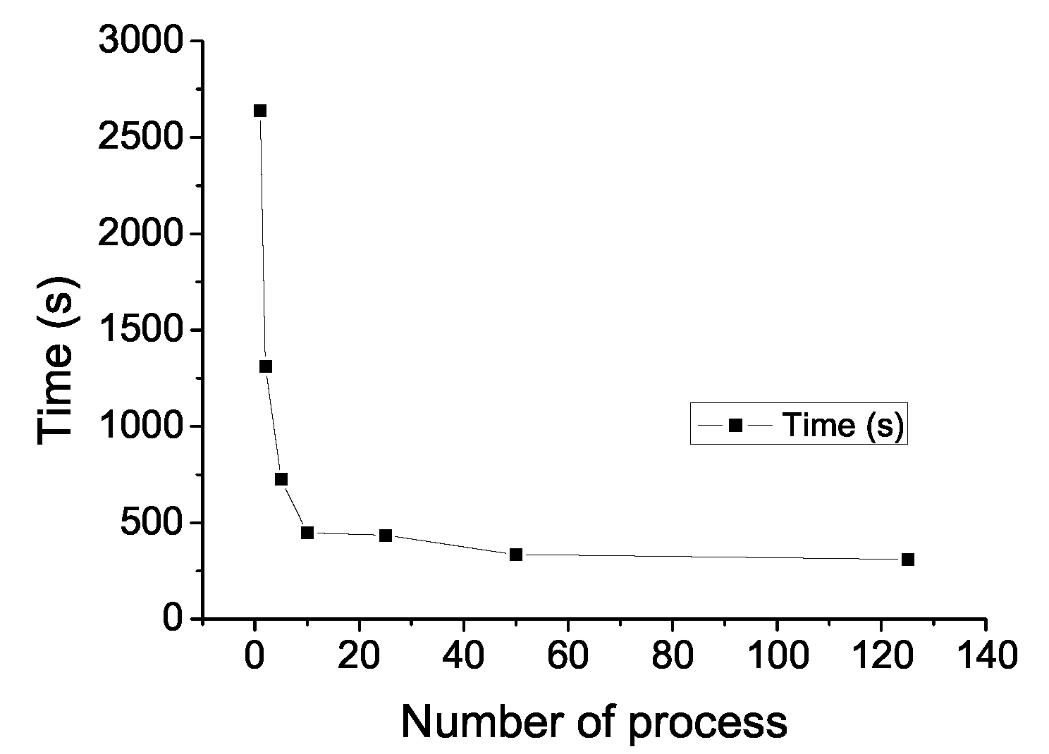
The execution time taken by the proposed parallel causality methodology applied to the identification and classification of natural scenery, for a total of 700 images, 6 different scenery, and varying the number of processes, are shown in Figure 20. These values were the average time taken for 200 executions. We can observe that the execution time decreased rapidly while increasing the number of processes, getting the best execution time when 125 concurrent processes were defined. With this configuration each process worked with 5 or 6 images, favoring the internal scheduling that used more efficiently the computer resources so that the sequential version execution time decreased by $88.9\%$.

7. Discussion

To find the texture causality relationships for characterizing a natural scenery, we found the necessity of GA implementation. With this solution, the automatic discrimination process for selecting the causal relationships that are important or relevant for the classification of the proposed scenery was successfully achieved. Compared to some of the articles in the literature, the possibility of our approach to perform the selection in an automatic way allows the study of the scenery classification problem considering more parameters. In this way, a larger number of scenery or base textures for future implementations of several purposes of texture classification could be taken into account considering the efficient methodology and evolutionary algorithm proposed in this work. This proposal could help in recognizing natural scenarios in the navigation of an autonomous car or possibly a drone, being an important element in the safety of autonomous vehicles navigation.

As we can see in Figure 17, the classification percentage obtained by means of the selected features for the evolutionary process surpasses those obtained by the manual selection version. This result is important because the representative causal relationships of the scenery are selected in such a way that they numerically escape the manual perspective; that is to say, in the manual selection strategy a non-significant threshold value is specified, such that any value lower than the threshold is set to zero, but evolutionary strategy turns out that some of these causal relationships are relevant to classify the scenery, marking differences with another similar scenery. From the causality theory applied to the image reading sequences, we are trying to infer the order of appearance of the textures typified in the base dictionary seeking to represent them as temporal visual reading that we see as a type of natural scenery.

8. Conclusions

In this paper a novel proposal for the use of the Wiener-Granger causality theory supported by a genetic algorithm was presented, along with the CBIR self-content analysis, applied for the identification and classification of 6 natural scenery: coast, forest, mountain, prairie, river/lake, and sky/cloud. Considering the new formulation it was possible to find a set of descriptors from the causality matrices in order to represent a scenery class, from a base set of reference textures, proposing a characterization of images based on the continuous appearance of textures within them; the base dictionary in this approach included the textures: Cloud, Sky, Rock, and Forest. Unlike others approaches, our methodology deals with the rotation and image noise considerations, and the results show excellent classification percentages.

Under this approach we have 100% image classification for the whole dataset, and the methodology provided the next good classification rate for ${180}^{\circ }$ rotation, and the sensitivity for intermediate rotation levels (${45}^{\circ }$, ${90}^{\circ }$), and had good results for the salt and pepper image noise.

In relation to the proposal performance, the design of a parallel computing algorithm was developed. A reduction in execution times was achieved using a 19-processor dual-core cluster server, and the MPI tool, reaching an 88.9% decrease of the sequential version execution time when 125 processes were launched.

Future work includes the study of performance of this proposal using other parallel architectures; e.g., the GPU technology could perform efficiently for the image feature extraction stage, as well as the implementation of other evolutionary algorithms, such as Genetic Programming in order to analyze all together the image textures looking to characterize the whole scenery and its associations with paradigm of visual comprehension.

References

- Gustavo, O. Evolutionary Computer Vision: The First Footprints, 1st ed.; Natural Computing Series; Springer: Berlin/Heidelberg, Germany, 2016. [Google Scholar]
- Nalwa, V.S. A Guided Tour of Computer Vision. Volume 1 of TA1632; Addison Wesley: Boston, MA, USA, 1993. [Google Scholar]
- Gonzalez, R.C.; Woods, R.E. Digital Image Processing; Addison-Wesley Longman Publishing Co., Inc.: Boston, MA, USA, 1992. [Google Scholar]
- Tyagi, V. Content-Based Image Retrieval: Ideas, Influences, and Current Trends, 1st ed.; Springer: Singapore, 2017. [Google Scholar]
- Benavides, C.; Villegas-Cortez, J.; Roman, G.; Aviles-Cruz, C. Reconocimiento de rostros a partir de la propia imagen usando técnica cbir. In Proceedings of the X Congreso Español sobre Metaheurísticas, Algoritmos Evolutivos y Bioinspirados (MAEB 2015), Merida Extremadura, Spain, 4–6 February 2015; pp. 733–740. [Google Scholar]
- Benavides, C.; Villegas-Cortez, J.; Roman, G.; Aviles-Cruz, C. Face classification by local texture analysis through cbir and surf points. IEEE Latin Am. Trans. 2016, 14, 2418–2424. [Google Scholar] [CrossRef]
- Granger, C.W. Investigating causal relations by econometric models and cross-spectral methods. Econometrica 1969, 37, 424–438. [Google Scholar] [CrossRef]
- Serrano-Talamantes, J.F.; Aviles-Cruz, C.; Villegas-Cortez, J.; Sossa-Azuela, J.H. Self organizing natural scene image retrieval. Expert Syst. Appl. Int. J. 2012, 40, 2398–2409. [Google Scholar] [CrossRef]
- Deb, K.; Kalyanmoy, D. Multi-Objective Optimization Using Evolutionary Algorithms; John Wiley & Sons, Inc.: New York, NY, USA, 2001. [Google Scholar]
- Vogel, J.; Schiele, B. Performance evaluation and optimization for content-based image retrieval. Pattern Recognit. 2006, 39, 897–909. [Google Scholar] [CrossRef]
- Oliva, A.; Torralba, A. Modeling the shape of the scene: A holistic representation of the spatial envelope. Int. J. Comput. Vis. 2001, 42, 145–175. [Google Scholar] [CrossRef]
- Begum, R.; Halse, S.V. The smart car parking system using gsm and labview. J. Comput. Math. Sci. 2018, 9, 135–142. [Google Scholar] [CrossRef]
- Blaifi, S.; Moulahoum, S.; Colak, I.; Merrouche, W. Monitoring and enhanced dynamic modeling of battery by genetic algorithm using labview applied in photovoltaic system. Electr. Eng. 2017, 100, 1–18. [Google Scholar] [CrossRef]
- Alam, A.; Jaffery, Z. A Vision-Based System for Traffic Light Detection: SIGMA 2018, Volume 1, pages 333–343. 01 2019. IEEE Latin Am. Trans. 2016, 14, 2418–2424. [Google Scholar]
- Baltruŝaitis, T.; Robinson, P.; Morency, L. Openface: An open source facial behavior analysis toolkit. In Proceedings of the 2016 IEEE Winter Conference on Applications of Computer Vision (WACV), Lake Placid, NY, USA, 7–10 March 2016; pp. 1–10. [Google Scholar]
- Sultana, M.G. A Content Based Feature Combination Method for Face Recognition; Springer: Heidelberg, Germany, 2013; Volume 226, pp. 197–206. [Google Scholar]
- Madhavi, D.; Patnaik, R. Genetic Algorithm-Based Optimized Gabor Filters for Content-Based Image Retrieval; Springer: Singapore, 2018; pp. 157–164. [Google Scholar]
- Desai, R.; Sonawane, B. Gist, Hog, and Dwt-Based Content-Based Image Retrieval for Facial Images; Springer: Singapore, 2017; Volume 468, pp. 297–307. [Google Scholar]
- Gao, J.; Yang, J.; Zhang, J.; Li, M. Natural scene recognition based on convolutional neural networks and deep boltzmannn machines. In Proceedings of the 2015 IEEE International Conference on Mechatronics and Automation (ICMA), Beijing, China, 2–5 August 2015; pp. 2369–2374. [Google Scholar]
- Meng, F.; Wang, X.; Shao, F.; Wang, D.; Hua, X. Energy-efficient gabor kernels in neural networks with genetic algorithm training method. Electronics 2019, 8, 105. [Google Scholar] [CrossRef]
- Vogel, J.; Schiele, B. Semantic modeling of natural scenes for content-based image retrieval. Int. J. Comput. Vis. 2007, 72, 133–157. [Google Scholar] [CrossRef]
- Traina, A.J.M.; Balan, A.G.R.; Bortolotti, L.M.; Traina, C. Content-based image retrieval using approximate shape of objects. In Proceedings of the 17th IEEE Symposium on Computer-Based Medical Systems, Bethesda, MD, USA, 25 June 2004; pp. 91–96. [Google Scholar]
- Dabbiru, L.; Aanstoos, J.V.; Ball, J.E.; Younan, N.H. Screening mississippi river levees using texture-based and polarimetric-based features from synthetic aperture radar data. Electronics 2017, 6, 29. [Google Scholar] [CrossRef]
- Liu, Y.; Zhang, D.; Lu, G.; Ma, W.Y. A survey of content-based image retrieval with high-level semantics. Pattern Recognit. 2007, 40, 262–282. [Google Scholar] [CrossRef]
- Zeng, P.; Li, Z.; Zhang, C. Scene Classification Using Spatial and Color Features. In Proceedings of the 8th International Conference on Intelligent Information Processing (IIP), Hangzhou, China, 17–20 October 2014; Volume AICT-432 of Intelligent Information Processing VII. Shi, Z., Wu, Z., Leake, D., Sattler, U., Eds.; Springer: Berlin/Heidelberg, Germany, 2014; pp. 259–268. [Google Scholar]
- Bressler, S.L.; Seth, A.K. Wiener-granger causality: A well established methodology. NeuroImage 2011, 58, 323–329. [Google Scholar] [CrossRef] [PubMed]
- Matias, F.S.; Gollo, L.L.; Carelli, P.V.; Bressler, S.L.; Copelli, M.; Mirasso, C.R. Modeling positive granger causality and negative phase lag between cortical areas. NeuroImage 2014, 99, 411–418. [Google Scholar] [CrossRef] [PubMed]
- Mannino, M.; Bressler, S.L. Foundational perspectives on causality in large-scale brain networks. Phys. Life Rev. 2015, 15, 107–123. [Google Scholar] [CrossRef] [PubMed]
- Zhang, H.; Li, X. Effective connectivity of facial expression network by using granger causality analysis. Parallel Process. Images Optim. Med. Imaging Process. 2013, 8920, 89200K. [Google Scholar]
- Friston, K. Causal modelling and brain connectivity in functional magnetic resonance imaging. PLoS Biol. 2009, 7, e1000033. [Google Scholar] [CrossRef] [PubMed]
- Kim, E.; Kim, D.S.; Ahmad, F.; Park, H. Pattern-based granger causality mapping in fmri. Brain Connect. 2013, 3, 569–577. [Google Scholar] [CrossRef] [PubMed]
- Fablet, R.; Bouthemy, P.; Pérez, P. Nonparametric motion characterization using causal probabilistic models for video indexing and retrieval. IEEE Trans. Image Process 2002, 11, 393–407. [Google Scholar] [CrossRef] [PubMed]
- Kular, D.; Ribeiro, E. Analyzing Activities in Videos Using Latent Dirichlet Allocation and Granger Causality; Springer International Publishing: Cham, Switzerland, 2015; pp. 647–656. [Google Scholar]
- Prabhakar, K.; Oh, S.; Wang, P.; Abowd, G.D.; Rehg, J.M. Temporal causality for the analysis of visual events. In Proceedings of the 2010 IEEE Conference on Computer Vision and Pattern Recognition (CVPR), San Francisco, CA, USA, 13–18 June 2010; pp. 1967–1974. [Google Scholar]
- Zhang, C.; Yang, X.; Lin, W.; Zhu, J. Recognizing human group behaviors with multi-group causalities. In Proceedings of the Proceedings of the The 2012 IEEE/WIC/ACM International Joint Conferences on Web Intelligence and Intelligent Agent Technology—Volume 03, WI-IAT ’12, Macau, China, 4–7 December 2012; pp. 44–48. [Google Scholar]
- Fan, Y.; Yang, H.; Zheng, S.; Su, H.; Wu, S. Video sensor-based complex scene analysis with granger causality. Sensors 2013, 13, 13685–13707. [Google Scholar] [CrossRef] [PubMed]
- Winner, N. The Theory of Prediction; McGraw-Hill: New York, NY, USA, 1958; Chapter 8. [Google Scholar]
- Barnett, L.; Seth, A.K. The {MVGC} multivariate granger causality toolbox: A new approach to granger-causal inference. J. Neurosci. Methods 2014, 223, 50–68. [Google Scholar] [CrossRef] [PubMed]
- Nag, S. Vector quantization using the improved differential evolution algorithm for image compression. Genet. Program. Evolv. Mach. 2019, 20, 187–212. [Google Scholar] [CrossRef] [Green Version]
- Shirali, A.; Kordestani, J.K.; Meybodi, M.R. Self-adaptive multi-population genetic algorithms for dynamic resource allocation in shared hosting platforms. Genet. Program. Evol. Mach. 2018, 19, 505–534. [Google Scholar] [CrossRef]
- Karpov, P.; Squillero, G.; Tonda, A. Valis: An evolutionary classification algorithm. Genet. Program. Evol. Mach. 2018, 19, 453–471. [Google Scholar] [CrossRef]
- Martínez, Y.; Trujillo, L.; Legrand, P.; Galvan-Lopez, E. Prediction of expected performance for a genetic programming classifier. Genet. Program. Evol. Mach. 2016, 17, 409–449. [Google Scholar] [CrossRef] [Green Version]
Figure 1.
Proposed general methodology applied for image recognition.
Figure 2.
Classical methodology of image classification.
Figure 3.
Example of segmentation texture zone in a natural scene.
Figure 4.
Learning and testing architecture for the classification system.
Figure 5.
A grid partition image example, every grid has a window of pixels size.
Figure 6.
Reading image example among the grid neighborhood of the image.
Figure 7.
Generation of a texture-based causality relationship matrix, , using the WGC analysis.
Figure 8.
The matrix generation process, for every th row ∈.
Figure 9.
The genome construction.
Figure 10.
Representation of a query image construction into N samples.
Figure 11.
Flowchart showing the general GA algorithm implementation. (a) Implementation of the proposed General flowchart GA, and (b) GA implementation for a particular s-scenery.
Figure 12.
Genetic operators application.
Figure 13.
The proposed parallel algorithm structure.
Figure 14.
Example of images with Gaussian, salt, and pepper noise of 1%, 3%, and 10%, respectively.
Figure 15.
Rotation degrees applied to the images set.
Figure 16.
Evolutionary texture causal relationship graphs resulted for each scenery.
Figure 17.
Classification results of our proposal using the GA, considering different noise type and rotation configurations.
Figure 18.
Technical efficiency measures of the best GA individuals for each scenery: (a) precision measure, (b) recall measure, (c) accuracy measure and (d) F1 score measure.
Figure 19.
Performance of the GA for the natural scenery contained in the NSDB.
Figure 20.
Performance of the parallel methodology algorithm.