A Vehicle Type Dependent Car-following Model Based on Naturalistic Driving Study

Abstract

In this paper, a car-following model considering the preceding vehicle type is proposed to describe the longitudinal driving behavior closer to reality. Based on the naturalistic driving data sampled in real traffic for more than half a year, the relation between ego vehicle velocity and relative distance was analyzed by a multi-variable Gaussian Mixture model, from which it is found that the driver following behavior is influenced by the type of leading vehicle. Then a Hidden Markov model was designed to identify the vehicle type. This car-following model was trained and tested by using the naturalistic driving data. It can identify the leading vehicle type, i.e., passenger car, bus, and truck, and predict the ego vehicle velocity and relative distance based on a series of limited historical data in real time. The experimental validation results show that the identification accuracy of vehicle type under the static and dynamical conditions are 96.6% and 83.1%, respectively. Furthermore, comparing the results with the well-known collision avoidance model and intelligent driver model show that this new model is more accurate and can be used to design advanced driver assist systems for better adaptability to traffic conditions.

1. Introduction

The topic of car-following behavior has become increasingly important in traffic engineering and safety research [1,2,3]. Modeling the car-following behavior more effectively and accurately is of great benefit to several application areas, such as simulation of microscopic traffic, development of advanced driving assistance systems, etc. [4,5,6]. In the existing models, the multi-variables, e.g. relative distance, relative velocity, ego vehicle velocity, leading vehicle velocity, and time headway are required overall or partially to describe the car-following behavior. Moreover, the car-following behavior of a driver is a non-linear system with a high dimension. Thus, a common following model with fixed parameters is no longer suitable for new applications with more intelligence and user friendliness.

In the current researches, classical car-following models are designed to characterize the interactional phenomena between the individual driver and the traffic, e.g., microscopic simulation [7,8]. These types of car-following models include the Gazis-Herman-Rothery (GHR) model, safety distance or collision avoidance (CA) model, linear models, action point models (AP), and Fuzzy logic-based models [1,9]. They can provide a real-time calculation for simulation because of the simplicity. Other kinds of car-following models aim to describe the driver behavior with the same reaction as a real human driver [10,11]. Thus, some empirical models used for simulation were modified to describe the driver behavior [12]. For example, Chen et al. conducted research on headway/spacing between two consecutive vehicles by considering it as a certain stochastic process to achieve better accuracy than CA [13]. Yang et al. modified Gipps’ model by formulating the car-following distance as a function of both the distance and the relative velocity between the leading and ego vehicle [14]. After calibration, the field data evaluation results show that this model has a higher accuracy than the original Gipps’ model. The Intelligent Driver Model (IDM) is one of the most widely used models, which attempts to eliminate the difference between the real situation and the preferred [15,16].

Recently, with the development of the intelligent learning algorithms based on big data, it is possible to construct a more accurate car-following model based on a great deal of naturalistic driving data [17,18,19,20,21,22,23,24]. Ye et al. found that time headway (THW) is different when a driver follows different vehicles [25]. In other words, the type of leading vehicle has an impact on the driving behavior [4]. However, the aforementioned models ignore this important factor, i.e., leading vehicle type. Thus, Aghabayk et al. established a car-following model that is applicable to a different but fixed vehicle type, i.e., passenger car and heavy vehicle [26]. This model was developed on the basis of the local linear model tree approach with Next Generation Simulation (NGSIM) data obtained from a U.S. freeway under congested traffic conditions. Although various researches on the analysis of car-following behavior have been conducted, little effort has been made to study the influence of leading vehicle type on the car-following process especially in real dynamical driving conditions.

To establish a vehicle type-dependent car-following model, a combined Gaussian mixture model (GMM) and a hidden Markov model (HMM) are used to analyze the naturalistic driving data to find a car-following model considering the leading vehicle type. The GMM is used to fit driver’s following behavior by using the expectation maximization algorithm. By this analysis, a joint probability density function describing the relation between ego velocity and relative distance is found. Combining the ego vehicle velocity and relative distance together to form the observation state and considering the leading vehicle type as a hidden one, we designed an identify algorithm, which can estimate the leading vehicle type by using HMM. Furthermore, to predict a driver’s following behavior with limited historical data, an algorithm with weighted expectation is proposed to realize its real time application. This model has the following advantages:

(1)

It has the ability to identify the leading vehicle type in real-time because the HMM hidden state can be predicted with limited historical data;

(2)

The prediction accuracy is ensured by training the model with a large number of naturalistic driving data;

(3)

Its responsiveness to dynamical conditions is achieved by estimating the optimum state of a car-following model based on historical data.

The rest of the paper is organized as follows: Section 2 introduces the data set used in this study; the idea and structure of this new car-following model are described in Section 3; how to obtain the model parameters based on the naturalistic data are explained in Section 4; the effectiveness of this model is validated in Section 5; Section 6 and Section 7 give out some applications and further discussions about this study; and Section 8 concludes the paper.

2. Car-Following Data Collection and Preprocessing

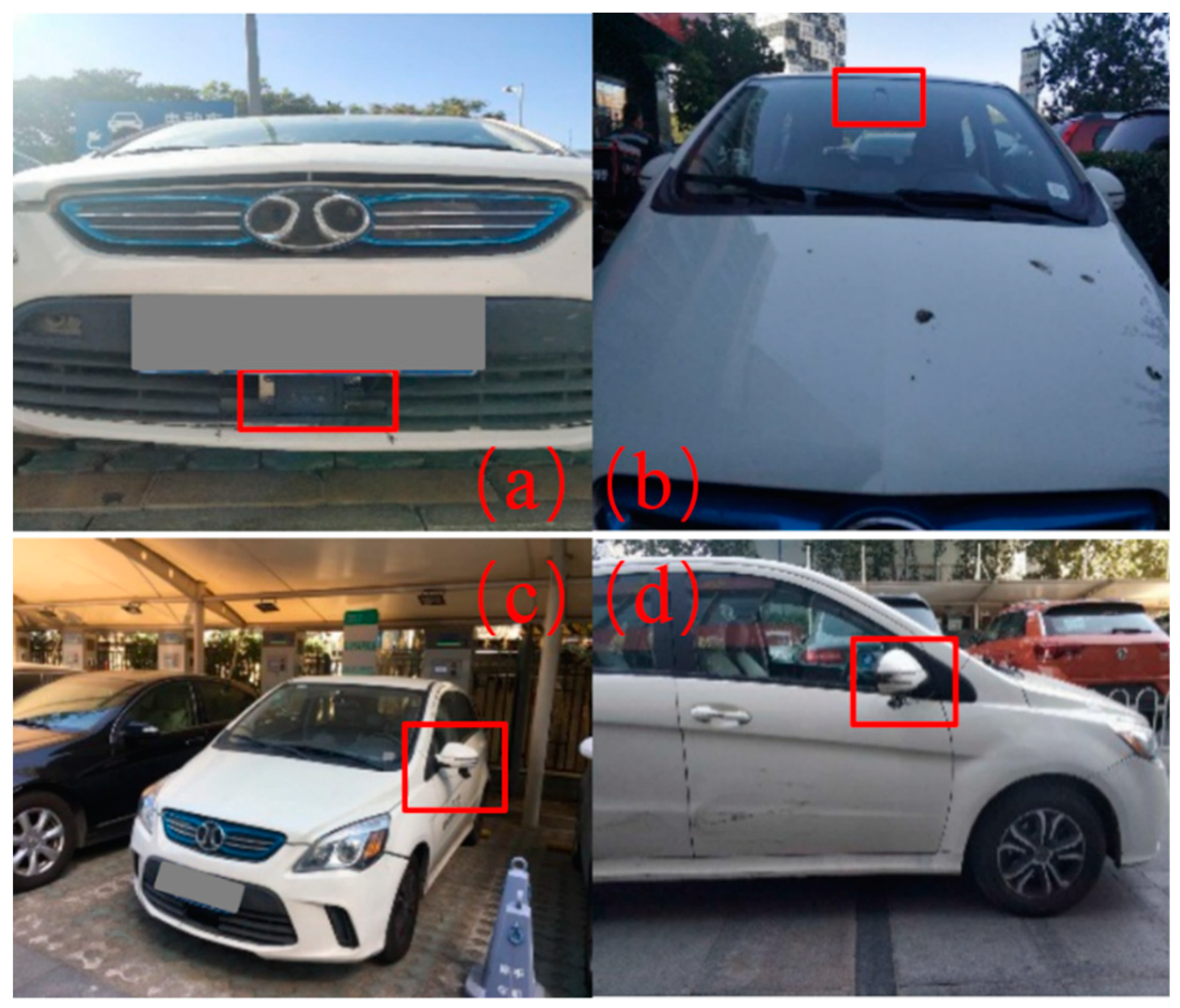
The naturalistic driving data is collected from a program of China Automotive Engineering Research Institute. In this database, 16 vehicles equipped with data acquisition systems were driven in Beijing, Shanghai, Tianjin, Chongqing, and Chengdu. As shown in Figure 1, these vehicles are equipped with a front-view camera, two side-view cameras and a front millimeter-wave (MMW) radar to measure the environment information including relative velocity, relative distance and leading vehicle type. The vision signal type of camera is LVDS, the resolution of image is $1280\times 720$ pixels, and the field angle is H52 and V43. The MMW radar type is ARS 408-21, produced by Continental, and has a detection range of 0–250 m. A Nvidia Jetson TX2 acts as the on-board computer to record and process the signals. The state of ego vehicle is acquired from the vehicle controller area network including the vehicle velocity, steering wheel angle, brake pressure, engine speed, acceleration, and gear position. The data acquisition vehicles have been driven for more than 50,000 km including both highways and city roads.

In this program, there is no restriction on driving routes. The data acquiring system is activated about 30 s after the engine starts and stops about 30 s before the engine stops. The sampling rate of the naturalistic driving data is 13 Hz. To guarantee that the drivers are not disturbed by the acquisition system, the equipped system is hidden and has no interaction with the driver. The driving behaviors, such as car-following, cut-in, and lane changing, are all recorded in the dataset. To choose the proper data, firstly, we define the car-following scenario, which should satisfy the following five criteria [5,27,28]:

a

Velocity range: Ego vehicle velocity, $v_{ego}$, should be more than 20 km/h, because the condition that the speed is less than 20 km/h contains a lot of stop-and-go scenarios.

b

Distance range: Relative distance, $y_r$, between the rear margin of the leading vehicle and the front margin of the ego vehicle should be less than 120 m. If this distance is greater than 120 m, the preceding vehicle has almost no effect on ego vehicle and this scenario is similar to the free-driving case.

c

Restrictions on leading vehicle: The leading vehicle should drive on the same lane with the ego vehicle.

d

Road curvature: The radius of the road should be larger than 150 m.

e

Time range: The ego vehicle should follow the leading vehicle consistently for more than 10 s. If the time is less than 10 s, there easily exists on-stable car-following scenarios, such as cut-in, cut-out and lane change.

After being filtered by the above five criteria, the extracted dataset of the stable car-following scenario is further divided into three categories according to the leading vehicle type:

• Car–car (C-C): a passenger car following a passenger car;
• Car–bus (C-B): a passenger car following a bus;
• Car–truck(C-T): a passenger car following a truck.

The statistical information of this dataset of car-following scenarios with different leading vehicle types is listed in

Table 1. Car-following dataset information.

Statistical Parameter	C-C	C-B	C-T
N	6965	723	305
Tc (s)	242,620	20,003	6655
Tac (s)	34.8	27.7	21.8

N: number of car-following cases. Tc: total car-following time. Tac: average car-following time.

.

3. Car-Following Model Design

Since a driver uses different following behaviors for different types of leading vehicles [25,29], a new model which can describe this feature is necessary. In this study, GMM is selected for modeling the following behavior of drivers because of the following two advantages:

(a)

It has already been demonstrated that GMM is effective in modeling the stochastic features of driver behavior [30,31];

(b)

It is a statistical model and the fundamental mechanism or detail of the driver response under internal exciting is not necessary [32].

Furthermore, under real traffic conditions, the leading vehicle may change frequently, so the model should have the ability to identify the leading vehicle type dynamically in real time. Unfortunately, the leading vehicle type can hardly be described by an explicit index with observed signals as its variables, because the interaction mechanism among the driver and environments is still not clear enough now. To overcome this difficulty, HMM is selected because it can describe the high dimension non-linear system and predict hidden states from a series of limited historical data [33]. And so in this study, GMM is used to establish the relation between the relative distance and ego velocity when following different vehicles. Then based on GMM, a HMM is designed to predict the leading vehicle type with historical data to guarantee the real time performance.

3.1. Car-following Behavior Fitted with Gaussian Mixture Model

In the GMM, the relative distance, $y_r$, and the ego vehicle velocity, $v_{ego}$, are selected as the exciting of the driver car-following behavior model [26]:

$$x=\left[v_{ego},y_r\right]$$

(1)

where $x$ is the input. According to the dataset of car-following described by Table 1, three independent GMMs are needed:

$$f_i\left(x_i;{\Theta }_i\right)={\displaystyle \sum }_{k=1}^K{\omega }_{i,k}{f}_{i,k}\left(x_i;{\theta }_{i,k}\right), i\in \left\{1,2,3\right\}$$

(2)

where $i$ is the type of leading vehicle and its value, 1, 2, 3, denotes passenger car, bus, and truck, respectively. The parameter ${\Theta }_i=\left[K,{\omega }_i,{\theta }_i\right]$, where $K$ is the component of GMM, ${\omega }_{i,k}$ is the weight of the k-th component of type $i$ and satisfying ${{\displaystyle \sum }}_{k=1}^K{\omega }_{i,k}=1$, ${\theta }_{i,k}=\left[{\mu }_{i,k},{\Sigma }_{i,k}\right]$ is the parameter of component $k$ of type $i$; ${\mu }_{i,k}$ and ${\Sigma }_{i,k}$ are the mean matrix and covariance matrix of the k-th component of type $i$ respectivly.

To identify the parameter values in (2), a revised Expectation Maximum (EM) algorithm is designed to solve the equation because the data used to train the parameters is truncated. It contains two steps called E step and M step respectively [34]:

E step: It is used to compute the posterior probability that $x$ belongs to the k-th component. Since the posterior probability remains unchanged with the truncated data, it is given by

$$p_k^{n+1}=\frac{{\pi }_k{f}_k\left(x_i\right)}{{{\displaystyle \sum }}_k{\pi }_k{f}_k\left(x_i\right)}$$

(3)

where $p_k^{n+1}$ is the probability of the condition that data $x_i$ belongs to the k-th component.

M step: This step is used to compute the maximum $\Theta$. The Lagrange multiplier is used and the original analytic equations are modified as follows to adapt to the truncated dataset:

$$\begin{array}{c}{\omega }_k^{n+1}=\frac{1}{N}{\displaystyle {\displaystyle \sum }_{n=1}^N}{p}_k^{n+1},\hspace{1em}{\mu }_k^{n+1}=\frac{{{\displaystyle \sum }}_n{p}_k^{n+1}{x}^{n+1}}{{{\displaystyle \sum }}_n{p}_k^{n+1}}-m_k,\\ {{\displaystyle \sum }}_k^{n+1}=\frac{{{\displaystyle \sum }}_n{p}_k^{n+1}\left(x-{\mu }_k^{n+1}\right){\left(x-{\mu }_k^{n+1}\right)}^T}{{{\displaystyle \sum }}_n{p}_k^{n+1}}+H_k\end{array}$$

(4)

The parameters, $m_k$ and $H_k$, in (4) are calculated by

$$m_k=M^1\left(0,{\Sigma }_k;\left[s-{\mu }_k,t-{\mu }_k\right]\right),\hspace{1em}{H}_k={\Sigma }_k-M^2\left(0,{\Sigma }_k;\left[s-{\mu }_k,t-{\mu }_k\right]\right)$$

(5)

where $M^1\left(\mu ,\Sigma ;\left[a,b\right]\right)$ and $M^2\left(\mu ,\Sigma ;\left[a,b\right]\right)$ are the moment and the second moment of Gaussian truncated range in $\left[a,b\right]$, respectively [34], $s=\min \left\{{\mu }_1,{\mu }_2,{\mu }_3\dots {\mu }_k\right\}$ and $t=\max \left\{{\mu }_1,{\mu }_2,{\mu }_3\dots {\mu }_k\right\}$.

The termination condition of the EM algorithm is set to be

$$L\left({\Theta }_i^{n+1}\right)-L\left({\Theta }_i^n\right)<ϵ$$

(6)

where $L\left({\Theta }_i^{n+1}\right)=log\left(f\left(x_i;{\Theta }_i^{n+1}\right)\right)$. The last parameter $K$ of GMM is determined by the Bayesian information criterion (BIC) because of its positive correlation with the computation burden [27]. The parameters are trained with the car-following dataset by using (3)–(5) interactively until the termination condition (6) is established.

3.2. Identification of Leading Vehicle Type with Hidden Markov Model

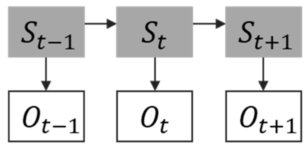
As shown in Figure 2, we define the hidden state, $S$, as the leading vehicle type, that is, $S=\left\{S_1,\dots S_t,\dots \right\}$, $t=1,2,\dots ,S_t\in \left\{1,2,3\right\}$. The value of hidden state, 1, 2, 3, represents passenger car, bus, and truck, respectively. The observation variable is $O=\left\{O_1,\dots ,O_t,\dots \right\}$, where $O_t=\left\{v_{ego,t},y_{r,t}\right\}$. Then the transfer probability and emission probability of the Markov process are defined as.

$$p\left(S_t|S_1,\dots ,S_{t-1},O_1,\dots ,O_{t-1}\right)=p\left(S_t|S_{t-1}\right),\hspace{1em}p\left(O_t|S_1,\dots ,S_t,O_1,\dots ,O_{t-1}\right)=p\left(O_t|S_t\right).$$

(7)

Furthermore, the transfer matrix of HMM, $A=\left[A_{i,j}\right]\in {ℝ}^{3\times 3}$, can be calculated by using the naturalistic driving dataset as

$$A_{i,j}=p\left(S_t=j,S_{t-1}=i\right)=\frac{T_{i,j}}{{\Sigma }_{j=1}^3{T}_{i,j}},\hspace{1em}{T}_{i,j}=\Sigma \left(M_i\to M_j\right)$$

(8)

where $M_i\in \left\{1,2,3\right\}$ and the value indicates passenger car, bus, and truck respectively; $M_i\to M_j$ represents a mode transition from $M_i$ to $M_j$; and $T_{i,j}$ is the total number of transitions. Since $O_t$ is continuous, the emission probability equals to $f\left(x_i;{\Theta }_i\right)$:

$$B\left(O_t\right)={\displaystyle \sum }_{k=1}^K{\omega }_k{B}_k\left(O_t\right)={\displaystyle \sum }_{k=1}^K\frac{{\omega }_k}{{\left(2\pi \right)}^{\frac{r}{2}}{\left|{\Sigma }_k\right|}^{\frac{1}{2}}}exp\{-\frac{1}{2}\left(O_t-{\mu }_k\right){\Sigma }_k^{-1}{\left(O_t-{\mu }_k\right)}^T\}$$

(9)

where $B\left(O_t\right)$ is the emission probability and r is the dimension of observation data. The initial probability, $\pi$, of the hidden state is defined as

$$\pi =\left[p\left(S_t=1\right)\hspace{1em}p\left(S_t=2\right)\hspace{1em}p\left(S_t=3\right)\right],\hspace{1em}p\left(S_t=i\right)=\frac{F_i}{{{\displaystyle \sum }}_{i=1}^3{F}_i},$$

(10)

where $F_i$ is the number of car-following conditions whose leading vehicle type is $i$. Then the best state sequence, $S_1^{*},\dots ,S_t^{*}$, to fit the historical data can be calculated by the Viterbi algorithm [35]:

$$S_t^{*}={\mathrm{argmax}}_{S^{*}\in S}\left(V_{t,S^{*}}\right),$$

(11)

$$V_{t,S^{*}}={\max }_{S^{*}\in S}\left(p\left(O_t|S_{t-1}^{*}\right)p\left(S_{t-1}^{*}|S^{*}\right)V_{t-1,S_{t-1}^{*}}\right)={\max }_{S^{*}\in S}\left(B_{S_{t-1}^{*}}\left(O_t\right)A_{S^{*},S_{t-1}^{*}}{V}_{t-1,S_{t-1}^{*}}\right)$$

(12)

The initial state used to solve the above optimal problem iteratively is set to be

$$V_{1,S^{*}}=p\left(O_1|S_1\right)\pi \left(S_1\right).$$

(13)

Then with a series of historical data, the optimal estimation of leading vehicle type can be obtained by using (7)–(13) [29]. When there is a new sample of car-following data, the observation state, i.e., the ego vehicle speed and relative distance, is calculated by the one-step prediction as

$${\widehat{O}}_{t+1}=\frac{1}{J}{\displaystyle \sum }_{j=0}^{2m}{\displaystyle \sum }_{k=1}^K{A}_k\left(S_{t+1},S_t\right){\omega }_k{B}_k\left(O_{t-j}\right)O_{t-j}=\frac{1}{J}{\displaystyle \sum }_{k=1}^K{A}_k\left(S_{t+1},S_t\right)E_k\left(B\left(O\right)\right)$$

(14)

where $O=\left\{O_{t-J+1},\dots O_t\right\}$ is the historical data, $E_k\left[B\left(O\right)\right]$ is the expectation of vehicle type k calculated by the data sequence $O$, and $J$ is the odd integer [36], which is a design parameter discussed in Section 4.2.

In summary, the model parameters, B, A, and $\pi$ are calculated according to (2), (8), and (10) using the car-following dataset, respectively. When using this model, the current leading vehicle type is identified by (11), using (11) and (14) interactively to predict.

4. Model Training

In this section, the car-following dataset set up in Section 2 is used to train the three GMMs to identify three types of leading vehicles respectively. The dataset is divided into a training and testing set with the ratio of 8:2.

4.1. Training of GMM

The component of GMM, K is given by [37]

$$BIC\left(K\right)=K\ln \left(n_c\right)-2\ln \left(L\left(\Theta \right)\right)$$

(15)

where $n_c$ is the number of training data and BIC is an increasing function of the error variance and K. Considering the complexity of the model and the computation burden, a model prefers a lower BIC [38]. Thus, $K$ is optimized by

$$K_{min}={\mathrm{argmin}}_K\left(BIC\left(K\right)\right)$$

(16)

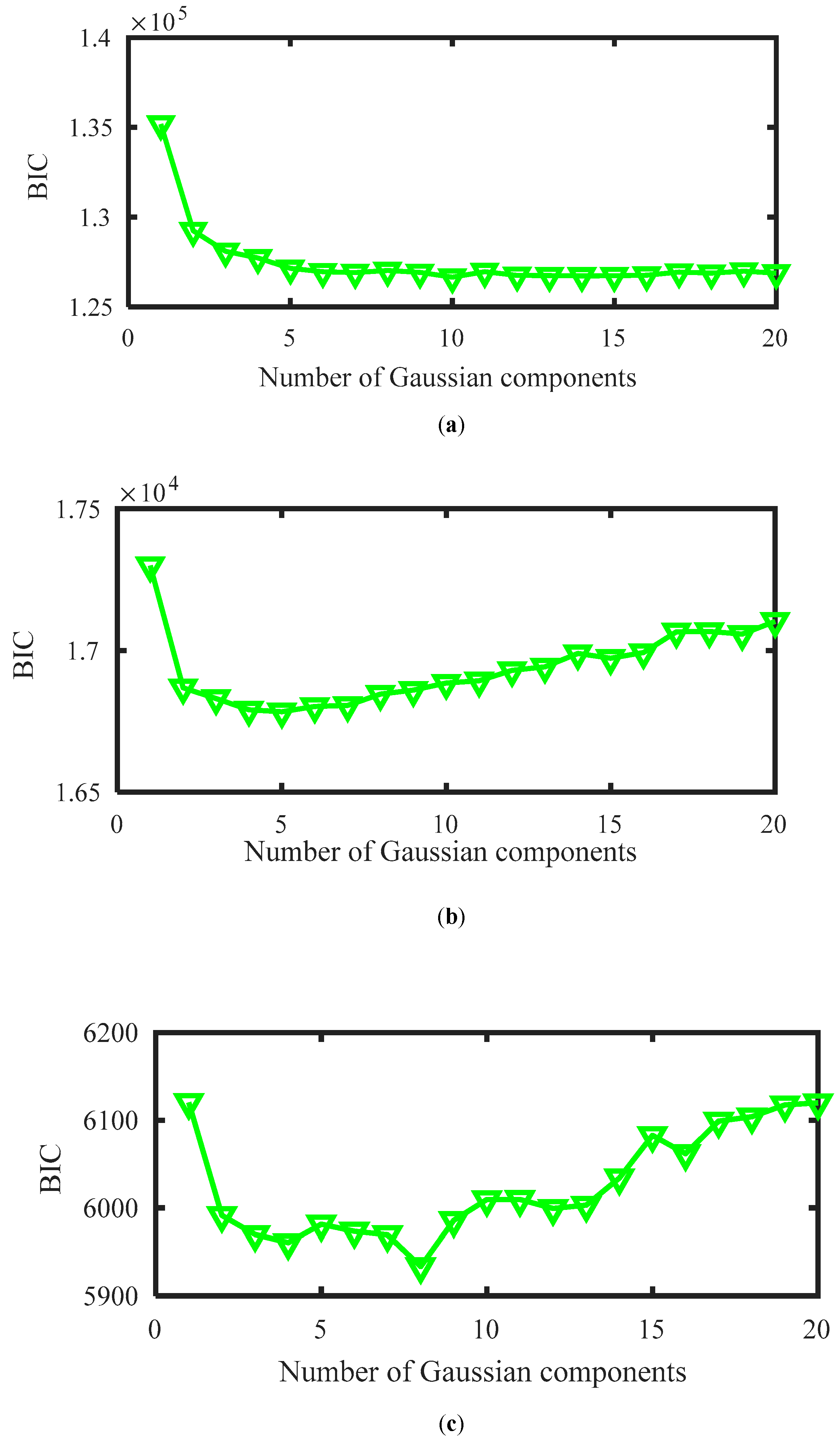
Let K increase from 1 to 20 step by step and then fit the components of GMM with the termination condition $ϵ={10}^{-8}$. The results of BIC are shown in Figure 3.

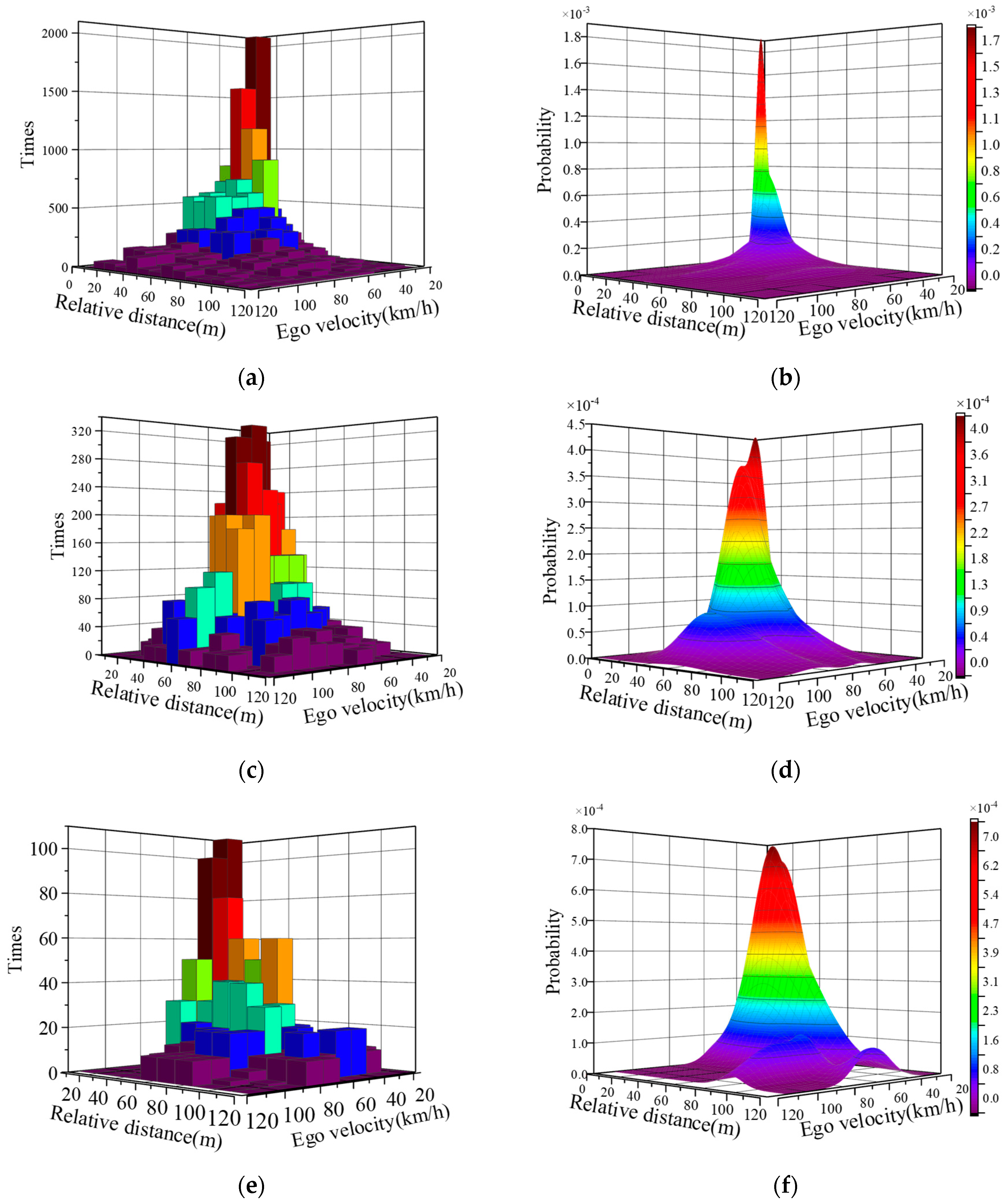
Normally, BIC decreases at the beginning when the value of the Gaussian component is small and will go up until reaching a big constant with the increasing value of the Gaussian component [38]. In Figure 3a, BIC decreases at the beginning and then almost holds after $K>5$. In Figure 3b,c, BIC decreases at the beginning and then goes up with the increasing $K$. The trend of BIC in Figure 3a–c is different, which is caused by the different amounts of training data. Normally, a larger amount of training data leads to a larger value of BIC. From (16), the value of K should be selected, ensuring the minimum value of BIC, and so the value of K for passenger car, bus, and truck is set to 10, 5, and 8, respectively. With the selected K, the raw data and trained GMM are shown in Figure 4.

From Figure 4, it is found that three raw data histograms have the same tendency with the fitted GMM surfaces. These distributions are mainly concentrated at the lower relative distance and lower ego velocity. The reason is that the raw data contains more than 75% city road data, about 20% highway data and the rest is country road or others. Furthermore, the distribution of data of different types of leading vehicle is also different. This implies that the driver-following behavior is influenced by the leading vehicle type, which should be considered when setting up the car-following model.

4.2. Prediction of Vehicle Type

With the trained GMMs, in this section, how to obtain the parameters in HMM are discussed. Firstly, the design parameter, J, is to indicate whether global or local features should be focused on [39]. In (14), J is odd when m is an integer. Considering the requirement of dynamic performance, a small m from 1 to 5 is considered and the corresponding $J=\left[3,5,7,9,11\right]$. With the testing data, the root mean squared error (RMSE) and root mean squared percentage error (RMSPE) are used to evaluate the model accuracy [40]:

$$RMSE=\sqrt{\frac{1}{N}{\displaystyle \sum }_i{\left({\widehat{y}}_i-y_i\right)}^2},\hspace{1em}RMSPE=\sqrt{\frac{1}{N}{\displaystyle \sum }_i{\left(\frac{{\widehat{y}}_i-y_i}{y_i+\delta }\right)}^2}$$

(17)

where ${\widehat{y}}_i$ and $y_i$ are the predicted value and the actual driving data respectively, $\delta$ is a small positive constant used to prevent zero divisor, and N is the size of data. The model accuracy under different values of J is shown in

Table 2. Model accuracy with different value of J.

J	Ego Velocity		Relative Distance
	RMSE (km/h)	RMSPE	RMSE (m)	RMSPE
3	0.1907	0.0097	0.0750	0.0119
5	0.2627	0.0133	0.1064	0.0169
7	0.3368	0.0170	0.1352	0.0213
9	0.4110	0.0206	0.1616	0.0254
11	0.4813	0.0241	0.1857	0.0291

. From Table 2, it is found that the minimum RMSE and RMSPE are both at $J=3$.

5. Model Testing

5.1. Identification Accuracy of Leading Vehicle Type

A statistical index is defined to evaluate the accuracy of the presented HMM for identification of a leading vehicle type [5]:

$$\eta =\frac{TT+FF}{TT+TF+FT+FF}$$

(18)

where TT is the number of conditions that HMM identifies the correct vehicle type, TF is the number of times that HMM takes the real type as others, FT is the number of times that HMM takes other types as the real one, and FF is the number of times that HMM identifies the non-specified type in the dataset correctly. Firstly, the static condition, under which the leading vehicle remains unchanged but its type is unknown, is selected to test the HMM identification ability. The average accuracy is shown in

Table 3. Accuracy of vehicle type identification.

Identification Accuracy	C-C	C-B	C-T	Average
$\eta$	98.7%	92.8%	98.2%	96.6%

.

Under the static condition, HMM shows a high level of performance of identification accuracy, which is 96.6%. When the leading vehicle type holds, the driver receives the same stimulus signal, thus the inner character of observation data, i.e., the relative distance and ego velocity, stay the same. In addition, the three truncated Gaussian mixture distributions have significant differences with each other as shown in Figure 4. That is why the leading vehicle type can be identified with a high level of accuracy.

5.2. Dynamical Condition

When driving on the road, the leading vehicle can hardly always be the same, and so dynamical test conditions are used to further validate the effectiveness of the proposed car-following model. Under this condition, the initial leading vehicle type, the time when the leading vehicle changes, and its duration are all unknown. Such dynamical conditions are more critical than the stable ones. The statistical accuracy is reported in

Table 4. Identification accuracy under dynamical conditions.

Identification Accuracy	C-C	C-B	C-T	Average
$\eta$	87.6%	81.2%	80.4%	83.1%

.

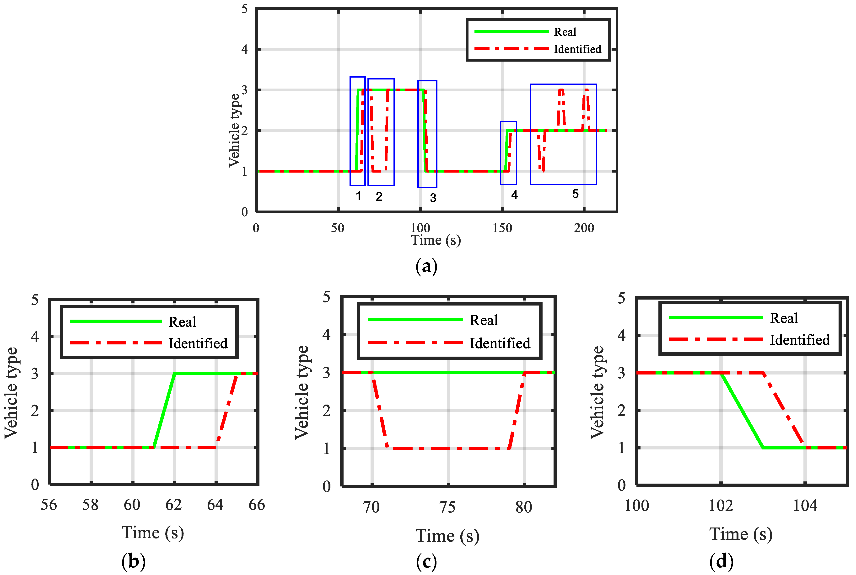
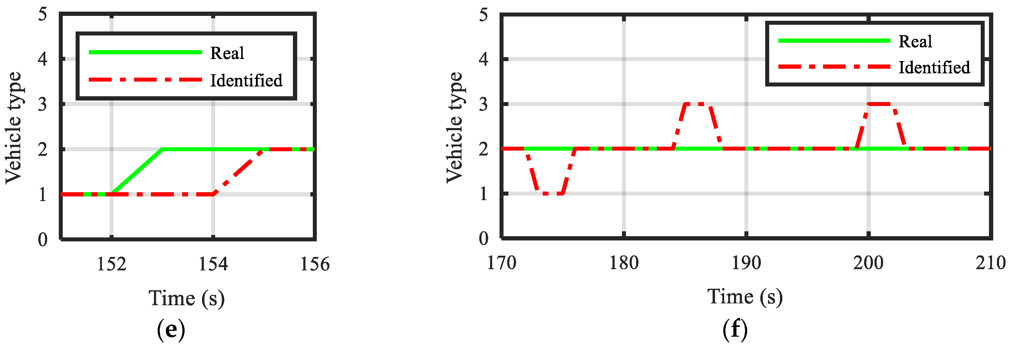
From Table 4, it is found that the identification accuracy of the passenger car is higher than others. The reason is that the training data of a passenger car is much larger. Thus, the corresponding component in GMM has a stronger ability and accuracy. The identification accuracy of the bus and truck is almost the same, because the driver has almost the same reaction when the leading vehicle is a truck or bus. Furthermore, compared with the results in Table 3, the accuracy decreases obviously because the change of leading vehicle type causes a time delay to the model. During the identification period, the same reaction may happen to different leading vehicles. Thus, the observation data will hide the missed information, which leads to misidentification. To show the details, a typical identification process is shown in Figure 5.

Figure 5b–e shows a time delay when the leading vehicle changes to another. The driver model needs a period of time to adapt to the new condition. Figure 5c,f shows an error identification, where the truck is misidentified as a passenger car and lasts about 10 s (Figure 5c). This is because the training data of C-T is far less than C-C, which cannot cover all possible driving conditions. In Figure 5f, the bus is misidentified as a passenger car or a truck. Besides the data size, another reason is that the truck and bus have similar shape features, which generates similar stimuli to the driver [4].

6. Application and Analysis

6.1. Driver Behavior Mimic Application

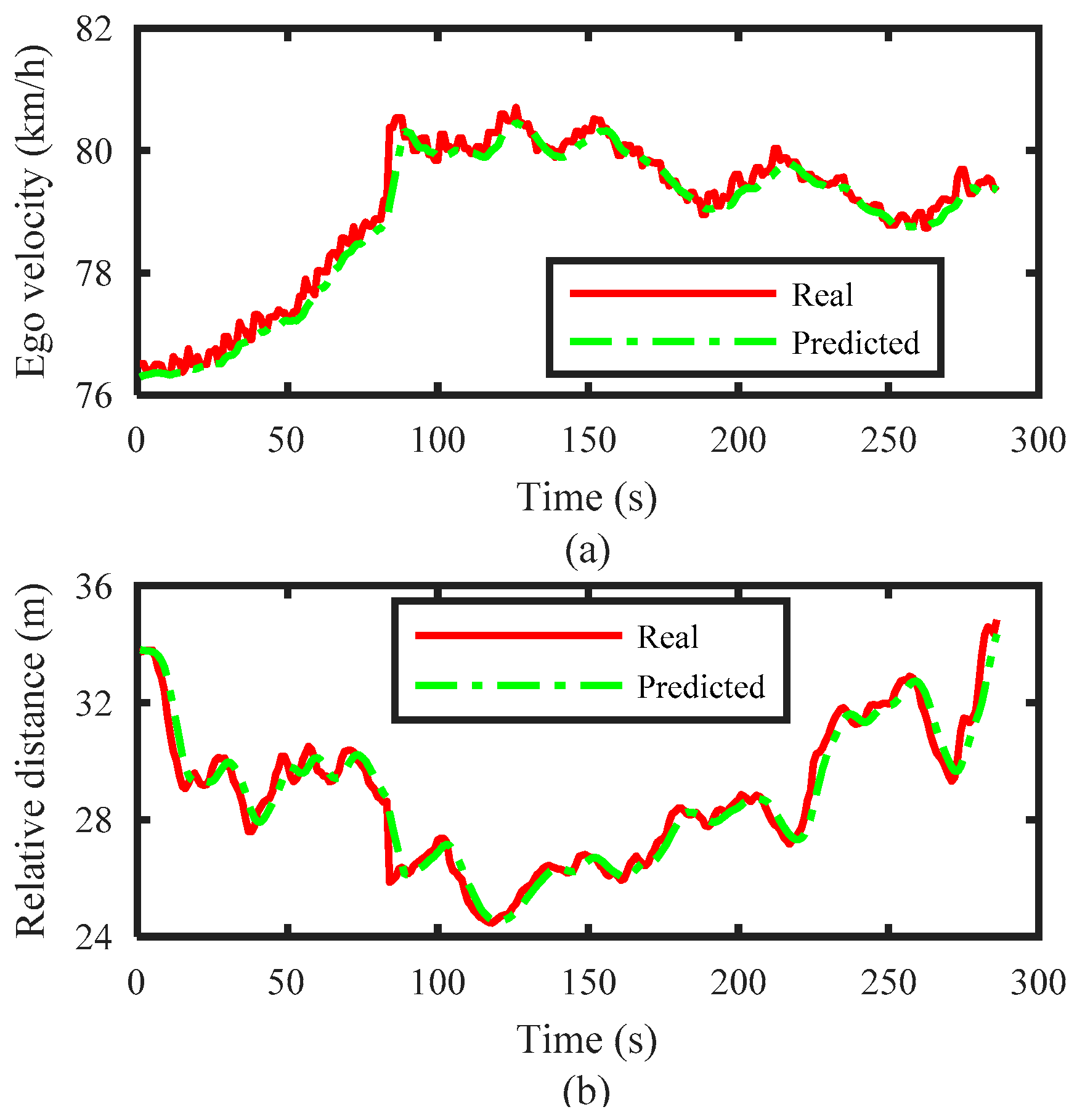
In order to evaluate the designed model, it has been applied to mimic the driver’s behavior. In this application, a 280 s naturalistic driving period is used and the results are shown in Figure 6. The results show that the predicted data is smoother than the real one and the model can predict the driver behavior finely with RMSE of velocity, and the relative distance is 0.21 km/h and 0.09 m.

6.2. Comparative Analysis

In this section, we compare the proposed model with other existing ones, namely the CA model and IDM. The CA model characterizes the safe distance, which is given by

$$\Delta Y\left(t-T\right)=\alpha v_{n-1}^2\left(t-T\right)+{\beta }_l{v}_n^2\left(t\right)+\beta v_n\left(t\right)+b_0$$

(19)

where, $\Delta Y$ is the relative distance, $v_{n-1}$ is the velocity of the ego vehicle and $v_n$ is the leading vehicle velocity. The parameters are set as T = 0.5, $\alpha =-0.00028,$ $\beta =$ 0.585, ${\beta }_l=0.00028$, and $b_0=4.1$ [1]. IDM can describe the desired following distance, which is given by

$$\Delta Y\left(v,\Delta v\right)=Y_0+vt+\frac{v\Delta v}{2\sqrt{ab}}$$

(20)

where, $v$ is the ego vehicle velocity and $\Delta v$ is the relative velocity. The parameters in (20) are set as $Y_0$ = 0.64, $v_0$ = 34, $T$ = 1.7, $a$ = 2, and $b$ = 20.14 [15,16,24]. The RMSE and RMSPE of relative distance are given in

Table 5. Accuracy comparison between existing models and the proposed model.

Leading Vehicle Type	Model	Relative Distance
		RMSE (m)	RMSPE
Passenger car	CA	1.3481	0.2360
	IDM	0.4192	0.0662
	Proposed	0.0750	0.0119
Bus	CA	2.3510	0.1524
	IDM	0.4986	0.1327
	Proposed	0.0820	0.0054
Truck	CA	14.5195	0.5791
	IDM	4.4358	0.1765
	Proposed	0.2281	0.0091

.

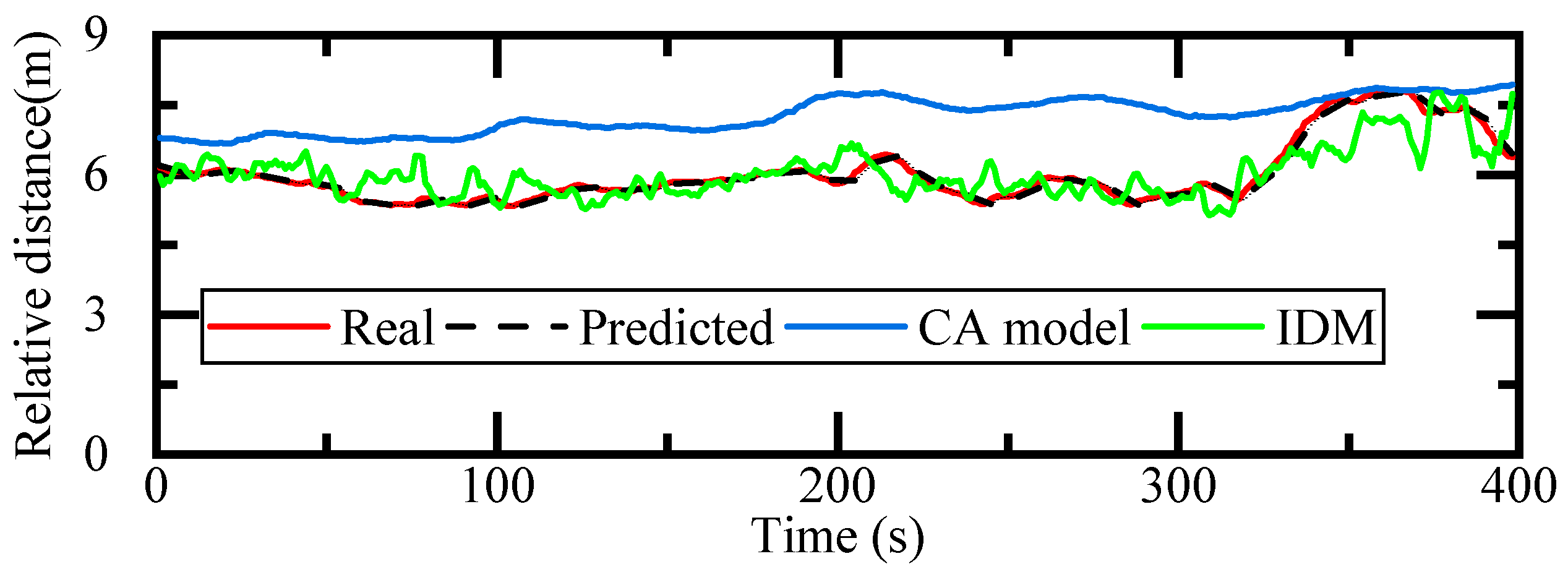
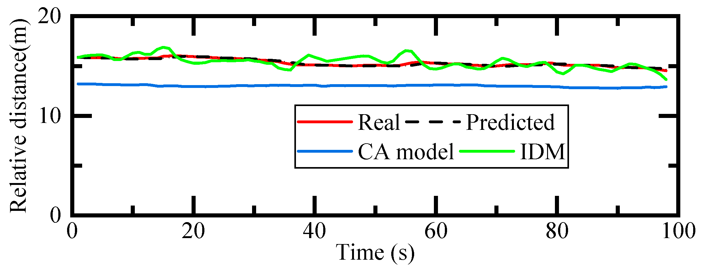
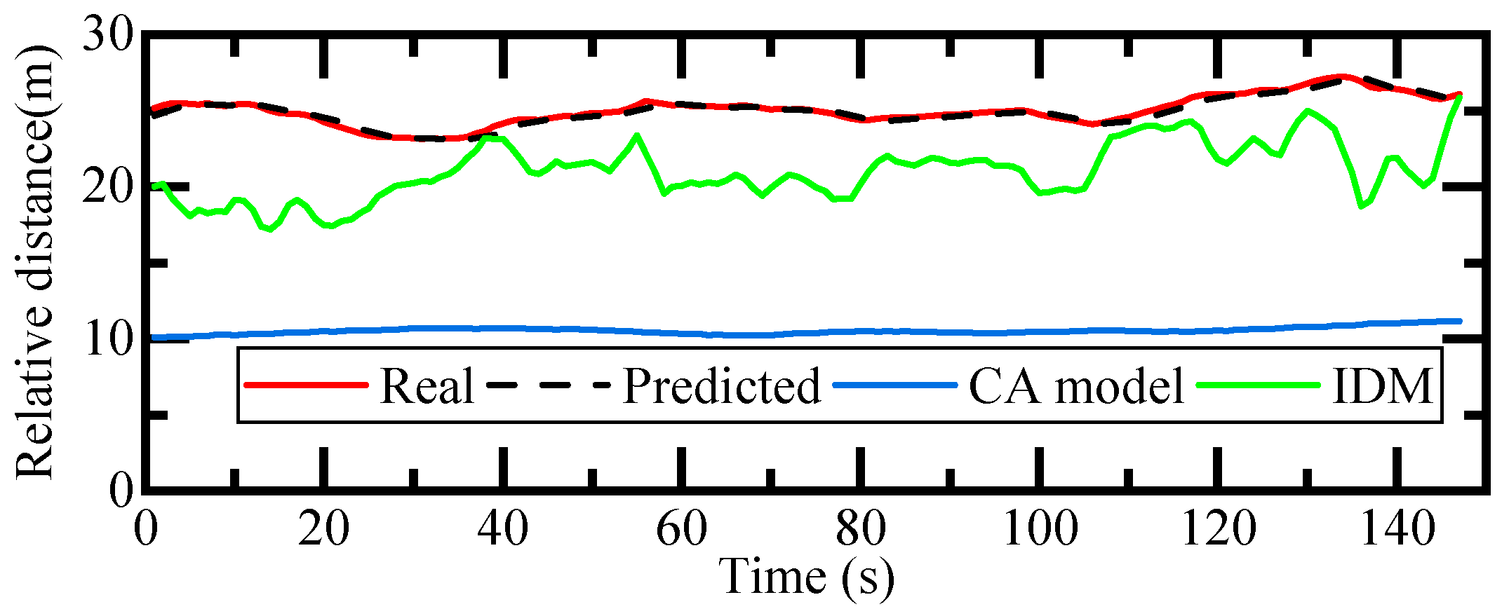
In Table 5, the accuracy of the proposed model is the best. The other two models have a comparatively larger RMSE and RMSPE. The reason is that the CA model is designed to keep a safer distance [1] and IDM is designed to eliminate the difference between the real situation and the preferred [15,16]. Therefore, they ignore the influence of the type of leading vehicle on the driver car-following behavior. Thus, they are not an appropriate choice for such application conditions. The comparison results indicate that the proposed model is suitable for mimicking the human driver behavior under such dynamic conditions. Some typical conditions are selected to show the details in Figure 7, Figure 8 and Figure 9.

The relative distance error of the proposed model is much smaller than others in Figure 7, Figure 8 and Figure 9. The output of IDM is closer to the real relative distance in Figure 7 and Figure 8. The CA model has the largest error of relative distance. In Figure 9, both CA and IDM output a smaller relative distance than the driver. The reason is that CA and IDM ignore the influence of leading vehicle type, which is mainly the outline of the leading vehicle [4]. A small-sized vehicle only blocks out a small portion of the traffic environment ahead. Comparatively, a larger vehicle easily causes critical accidents. Therefore, when following a passenger car, the human driver is more aggressive and keeps with the vehicle closer. On the contrary, if the leading vehicle is a bus or a truck, the proposed model keeps a larger relative distance with the preceding vehicle than CA and IDM (Figure 9).

7. Discussion and Future Work

From the above-mentioned analysis, it is found that the proposed model can mimic human driver driving behavior, and the proposed model has a high level of accuracy of leading vehicle type identification. In this paper, we mainly focused on whether the different leading vehicle types have an influence on car-following behavior. However, individuals’ driving style were not considered. Potential directions in future work are discussed as follows.

7.1. Influence of Data Components

Driving on the city road and highway road are different driving styles. In this work, the model does not divide naturalistic driving data into city road, highway, and others. In extraction data, raw data contains more than 75% city road data, about 20% highway data, and the rest of the data is country road or others. In this data, the vehicle also keeps a lower velocity and a shorter relative distance. Thus, the proposed model prefers to fit a city road or low velocity driving condition. For the reason given above, the data components need to be divided into suitable parts in future research work.

7.2. Influence of Individual Driving Style

Car-following behavior is influenced by the driver’s personal characteristics. First, driving years of a driver can directly affect his or her driving habits. For example, a driver with more experience will demonstrate a more confident driving style. A driving condition which is easy for a seasoned driver, may be perceived to be quite difficult by a novice driver. Such a performance difference will make an influence on the model. Therefore, a historical data-based model method may solve the problem in future work.

7.3. Applications in Future Works

This paper proposed a novel car-following model which considered the leading vehicle type. This model can apply to a human-friendly driver assist system. Each leading vehicle type corresponds to a different car-following strategy. For example, this model can be applied to a human-friendly Autonomous Emergency Braking (AEB) system, thus the driver will be warned at different velocities and different relative distances with the different leading vehicle types. In other words, with the same velocity and relative distance, the AEB system will warn the driver earlier if the leading vehicle is a truck compared to that of a bus or car. The proposed model can also be applied to Adaptive Cruise Control (ACC) system. In the car-following condition with different leading vehicle types, the model can calculate the relative distance and velocity of the leading vehicle to mimic human driver behavior to control the vehicle.

8. Conclusions

This paper has developed a GMM-HMM model for learning, identify leading vehicle type, and predicting ego vehicle velocity and relative distance in a car-following scenario. The proposed model is formulated from sample data. In the proposed model, ego vehicle velocity and relative distance are used. The relation between ego vehicle velocity and relative distance are fitted by a truncated GMM. The leading vehicle type is identified in real-time by a hidden Markov model. The identified vehicle types are passenger car, bus, and truck. Ego vehicle next state is predicted with an expectation of a series of historical driving data. The experiment’s results show that the identification accuracy of a single leading vehicle type and changing leading vehicle type are 96.6% and 83.1% on average, respectively. Compared to the proposed model with the existing CA model and IDM, the results show that the proposed model can mimic the driver behavior better than the CA model and IDM. The model is more suitable for a real car-following condition with a changing leading vehicle type.

In summary, the model has two advantages. (1) It can identify the leading vehicle type in real-time with a high level of accuracy; (2) the model has a strong ability to mimic driver car-following behavior in nature driving conditions.

References

- Brackstone, M.; Mcdonald, M. Car-following: a historical review. Transp. Res. Part F Traffic Psychol. Behav. 1999, 2, 181–196. [Google Scholar] [CrossRef]
- Martinez, C.M.; Heucke, M.; Wang, F.-Y.; Gao, B.; Cao, D. Driving Style Recognition for Intelligent Vehicle Control and Advanced Driver Assistance: A Survey. IEEE Trans. Intell. Transp. Syst. 2018, 19, 666–676. [Google Scholar] [CrossRef]
- Rahman, M.; Chowdhury, M.; Khan, T.; Bhavsar, P. Improving the Efficacy of Car-Following Models with a New Stochastic Parameter Estimation and Calibration Method. IEEE Trans. Intell. Transp. Syst. 2015, 16, 1–13. [Google Scholar] [CrossRef]
- Pariota, L.; Galante, F.; Bifulco, G.N.; Luigi, P. The impact of the leading vehicle type on car-following behaviours. In Proceedings of the International Conference on Models and Technologies for Intelligent Transportation Systems (MT-ITS), Budapest, Hungary, 3–5 June 2015; pp. 30–37. [Google Scholar]
- Wang, W.; Xi, J.; Zhao, D. Learning and Inferring a Driver’s Braking Action in Car-Following Scenarios. IEEE Trans. Veh. Technol. 2018, 67, 3887–3899. [Google Scholar] [CrossRef]
- Kesting, A.; Treiber, M.; Schönhof, M.; Helbing, D. Adaptive cruise control design for active congestion avoidance. Transp. Nat. Res. C Emerg. Technol. 2008, 16, 668–683. [Google Scholar] [CrossRef]
- Jin, S.; Huang, Z.; Tao, P.; Wang, D. Car-Following Theory of Steady-State Traffic Flow. Oper. Res. 1959, 7, 499–505. [Google Scholar]
- Gipps, P. A behavioural car-following model for computer simulation. Transp. Nat. Res. B Methodol. 1981, 15, 105–111. [Google Scholar] [CrossRef]
- Oh, C.; Kim, T. Estimation of rear-end crash potential using vehicle trajectory data. Anal. Prev. 2010, 42, 1888–1893. [Google Scholar] [CrossRef] [PubMed]
- Bifulco, G.N.; Pariota, L.; Simonelli, F.; Di Pace, R. Development and testing of a fully Adaptive Cruise Control system. Transp. Nat. Res. C Emerg. Technol. 2013, 29, 156–170. [Google Scholar] [CrossRef]
- Kuge, N.; Yamamura, T.; Shimoyama, O.; Liu, A. A Driver Behavior Recognition Method Based on a Driver Model Framework; SAE Technical Paper Series; Institute of Transportation Library: Berkeley, CA, USA, 2000. [Google Scholar]
- Wu, Z.; Liu, Y.; Pan, G. A Smart Car Control Model for Brake Comfort Based on Car Following. IEEE Trans. Intell. Transp. Syst. 2009, 10, 42–46. [Google Scholar]
- Chen, X.; Li, L.; Zhang, Y. A Markov Model for Headway/Spacing Distribution of Road Traffic. IEEE Trans. Intell. Transp. Syst. 2010, 11, 773–785. [Google Scholar] [CrossRef]
- Yang, D.; Yu, D.; Yang, F.; Pu, Y.; Zhu, L.-L. An enhanced safe distance car-following model. J. Shanghai Jiaotong Univ. 2014, 19, 115–122. [Google Scholar] [CrossRef] [Green Version]
- Kesting, A.; Treiber, M. Calibrating car-following models by using trajectory data methodological study. Transp. Res. Rec. J. Transp. Res. Board 2008, 2088, 148–156. [Google Scholar] [CrossRef]
- Zhu, M.; Wang, X.; Tarko, A.; Fang, S. Modeling car-following behavior on urban expressways in Shanghai: A naturalistic driving study. Transp. Nat. Res. C Emerg. Technol. 2018, 93, 425–445. [Google Scholar] [CrossRef]
- Hao, S.; Yang, L.; Shi, Y. Data-driven car-following model based on rough set theory. IET Intell. Syst. 2018, 12, 49–57. [Google Scholar] [CrossRef]
- Khodayari, A.; Ghaffari, A.; Kazemi, R.; Braunstingl, R. A Modified Car-Following Model Based on a Neural Network Model of the Human Driver Effects. IEEE Trans. Syst. Man Cybern. Nat. Res. A Syst. Hum. 2012, 42, 1440–1449. [Google Scholar] [CrossRef]
- Pourabdollah, M.; Bjarkvik, E.; Furer, F.; Lindenberg, B.; Burgdorf, K. Calibration and evaluation of car following models using real-world driving data. In Proceedings of the IEEE 20th International Conference on Intelligent Transportation Systems (ITSC), Yokohama, Japan, 16–19 October 2017. [Google Scholar]
- Wang, X.; Jiang, R.; Li, L.; Lin, Y.; Zheng, X.; Wang, F.-Y. Capturing Car-Following Behaviors by Deep Learning. IEEE Trans. Intell. Transp. Syst. 2018, 19, 910–920. [Google Scholar] [CrossRef]
- Saffarian, M.; De Winter, J.C.F.; Happee, R. Enhancing Driver Car-Following Performance with a Distance and Acceleration Display. IEEE Trans. Hum. Mach. Syst. 2013, 43, 8–16. [Google Scholar] [CrossRef]
- Jin, P.J.; Yang, D.; Ran, B. Reducing the Error Accumulation in Car-Following Models Calibrated with Vehicle Trajectory Data. IEEE Trans. Intell. Transp. Syst. 2014, 15, 148–157. [Google Scholar] [CrossRef]
- Higgs, B.; Abbas, M. Segmentation and Clustering of Car-Following Behavior: Recognition of Driving Patterns. IEEE Trans. Intell. Transp. Syst. 2015, 16, 81–90. [Google Scholar] [CrossRef]
- Zhu, M.; Wang, X.; Wang, Y. Human-like autonomous car-following model with deep reinforcement learning. Transp. Nat. Res. C Emerg. Technol. 2018, 97, 348–368. [Google Scholar] [CrossRef]
- Ye, F.; Zhang, Y. Vehicle Type–Specific Headway Analysis Using Freeway Traffic Data. Transp. Rec. J. Transp. Nat. Res. 2009, 2124, 222–230. [Google Scholar] [CrossRef]
- Aghabayk, K.; Sarvi, M.; Forouzideh, N.; Young, W. New Car-Following Model considering Impacts of Multiple Lead Vehicle Types. Transp. Rec. J. Transp. Nat. Res. 2013, 2390, 131–137. [Google Scholar] [CrossRef]
- Chen, B.; Zhao, D.; Peng, H. Evaluation of automated vehicles encountering pedestrians at unsignalized crossings. In Proceedings of the IEEE Intelligent Vehicles Symposium (IV), Los Angeles, CA, USA, 11–14 June 2017; pp. 1679–1685. [Google Scholar]
- Dozza, M.; Bärgman, J.; Lee, J.D. Chunking: A procedure to improve naturalistic data analysis. Anal. Prev. 2013, 58, 309–317. [Google Scholar] [CrossRef] [Green Version]
- Aghabayk, K.; Sarvi, M.; Young, W. Understanding the Dynamics of Heavy Vehicle Interactions in Car-Following. J. Transp. Eng. 2012, 138, 1468–1475. [Google Scholar] [CrossRef]
- Pariota, L.; Bifulco, G.N.; Brackstone, M. A Linear Dynamic Model for Driving Behavior in Car Following. Transp. Sci. 2016, 50. [Google Scholar] [CrossRef]
- Jiang, R.; Hu, M.-B.; Zhang, H.; Gao, Z.-Y.; Jia, B.; Wu, Q.-S. On some experimental features of car-following behavior and how to model them. Transp. Nat. Res. B Methodol. 2015, 80, 338–354. [Google Scholar] [CrossRef] [Green Version]
- Lefèvre, S.; Carvalho, A.; Borrelli, F. A Learning-Based Framework for Velocity Control in Autonomous Driving. IEEE Trans. Autom. Sci. Eng. 2016, 13, 1–11. [Google Scholar] [CrossRef]
- Angkititrakul, P.; Terashima, R.; Wakita, T. On the Use of Stochastic Driver Behavior Model in Lane Departure Warning. IEEE Trans. Intell. Transp. Syst. 2011, 12, 174–183. [Google Scholar] [CrossRef]
- Lee, G.; Scott, C. EM algorithms for multivariate Gaussian mixture models with truncated and censored data. Comput. Stat. Data Anal. 2012, 56, 2816–2829. [Google Scholar] [CrossRef] [Green Version]
- Viterbi, A. Error bounds for convolutional codes and an asymptotically optimum decoding algorithm. IEEE Trans. Inf. Nat. Theory 1967, 13, 260–269. [Google Scholar] [CrossRef]
- Yuan, Y.; Liu, X. Municipal waste generation forecasting based on improved hidden markov model. Ind. Eng. Manag. 2014, 19, 52–56. [Google Scholar]
- Liu, S.; Sa, R.; Maguire, O.; Minderman, H.; Chaudhary, V. Spot counting on fluorescence in situ hybridization in suspension images using Gaussian mixture model. Image Process. 2015, 9413. [Google Scholar] [CrossRef]
- Zhang, X.-B.; Qian, R.-H. Research on technical state evaluation of Vehicle Equipment based on BIC cluster analysis. In Proceedings of the 2nd International Conference on Big Data Analysis (ICBDA), Beijing, China, 10–12 March 2017; pp. 303–306. [Google Scholar]
- Nhita, F.; Saepudin, D.; Adiwijaya; Wisesty, U.N. Comparative Study of Moving Average on Rainfall Time Series Data for Rainfall Forecasting Based on Evolving Neural Network Classifier. In Proceedings of the 3rd International Symposium on Computational and Business Intelligence (ISCBI), Bali, Indonesia, 7–9 December 2015. [Google Scholar]
- Meng, Q.; Weng, J. An improved cellular automata model for heterogeneous work zone traffic. Transp. Nat. Res. C Emerg. Technol. 2011, 19, 1263–1275. [Google Scholar] [CrossRef]
Figure 1.
Data acquisition equipment mounted on the vehicle. Figure (a) shows the millimeter wave radar. Figures (b–d) show the cameras.
Figure 2.
HMM graph model.
Figure 3.
BIC value: (a) car, (b) bus, (c) truck.
Figure 4.
Comparison of raw data and Gaussian mixture model. (a) Car: raw data, (b) Car: Gaussian mixture model, (c) Bus: raw data, (d) Bus: Gaussian mixture model, (e) Truck: raw data, (f) Truck: Gaussian mixture model.
Figure 5.
Typical condition test results of leading vehicle type changing. (a) is a full figure. (b)–(f) are zoomed in to the five sections of the full figure in (a).
Figure 6.
The application results of driver behavior mimic.
Figure 7.
Results when following a passenger car.
Figure 8.
Results when following a bus.
Figure 9.
Results when following a truck.