TARCS: A Topology Change Aware-Based Routing Protocol Choosing Scheme of FANETs


1
Key Laboratory of Microwave Remote Sensing, National Space Science Center, Chinese Academy of Sciences, Beijing 100190, China
2
University of Chinese Academy of Sciences, Beijing 100094, China
*
Author to whom correspondence should be addressed.
Electronics 2019, 8(3), 274; https://doi.org/10.3390/electronics8030274
Submission received: 21 December 2018
/
Revised: 16 February 2019
/
Accepted: 21 February 2019
/
Published: 2 March 2019
(This article belongs to the Special Issue Mobile Oriented Future Internet (MOFI): Architectural Designs and Experimentations)
Abstract
:The rapid change of topology is one of the most important factors affecting the performance of the routing protocols of flying ad hoc networks (FANETs). A routing scheme suitable for highly dynamic mobile ad hoc networks is proposed for the rapid change of topology in complex scenarios. In the scheme moving nodes sense changes of the surrounding network topology periodically, and the current mobile scenario is confirmed according to the perceived result. Furthermore, a suitable routing protocol is selected for maintaining network performances at a high level. The concerned performance metrics are packet delivery ratio, network throughput, average end-to-end delay and average jitter. The experiments combine the random waypoint model, the reference point group mobility model and the pursue model to a chain scenario, and simulate the large changes of the network topology. Results show that an appropriate routing scheme can adapt to rapid changes in network topology and effectively improve network performance.
1. Introduction
Mobility is one of the most prominent features of mobile ad hoc networks (MANETs) and one of the important factors affecting network performance. Being a typical subset of MANETs, the node mobility in flying ad hoc networks (FANETs) [1,2,3] is stronger and severely impacts the network performance (Figure 1).
FANET has some unique characteristics compared to MANET and VANET (Table 1). In FANETs, high-speed moving nodes usually need to complete multiple tasks, such as search/exploration, reconnaissance/patrol, or target tracking. Different task scenarios could have corresponding node mobility models [1]. When the task changes, the node mobility mode (such as node motion speed, direction, distance, etc.) changes accordingly, which will cause the network topology to change rapidly and seriously affect the network performance.
The main research object of this paper is highly dynamic FANETs. Specifically, it corresponds to the FANETs listed in Table 1 in which the nodes move fast and the network topology changes drastically.
The characteristics of the FANETs discussed in this paper are: small and medium-sized networks, high mobility nodes far from the ground at high altitudes, sufficient node energy and frequent network topology changes.
In practical applications, FANETs encounter different application scenarios when nodes complete complex tasks. Nodes move in different ways in different scenarios, which causes large changes in the network topology. Traditionally, nodes cannot perceive this change, nor can they adapt quickly to it, so the network performance will deteriorate dramatically. The main purpose of this paper is to find a method by which nodes in a network can perceive changes of topology and adjust the routing strategy appropriately when the topology changes greatly, so that the network performance could be maintained at a high level. The most concerned network performance is the packet delivery ratio, followed by the average end-to-end delay, the average jitter, and finally the network throughput.
Many routing protocols have been proposed for mobile ad hoc networks [4]. Each protocol has its own characteristics and application scenarios. For example, the Optimized Link State Routing Protocol (OLSR) [5] is suitable for high-density MANETs, and the Destination-Sequenced Distance-Vector Routing (DSDV) [6] is more suitable for small-scale MANETs. When the scenario is complex and the network topology changes rapidly, a single routing protocol cannot meet the requirements of the variable node mobility mode, nor can network performance be guaranteed. Accurate perception of the surrounding environment and appropriate adjustment strategies of nodes have become the trends of adaptive routing protocols with the increasing requirements of quality of service (QoS). In response to the above objectives, this paper proposes a solution for choosing routing protocols in highly dynamic FANETs, namely TARCS (topology change aware-based routing protocol choosing scheme). The TARCS scheme is divided into the following steps:
Firstly, a topology change sensing method is proposed, which can measure the topology change between nodes of a high dynamic FANET, and a mobility metric TCD, the topology change degree with several levels is defined to quantify the perceived results.
Secondly, a heuristic routing strategy of FANETs is proposed using the measurement results of the sensing method. The policy compares the measured topology change result with the threshold reference value, determines the current node movement mode, and appropriately adjusts the routing protocol used in the network, so that the network routing protocol is more suitable for the changed mobile scenario, and finally the purpose of improving network performance in highly dynamic topology is achieved.
Simulations show that compared with traditional practices, the proper use of TARCS in highly dynamic MANETs in complex scenarios can effectively improve some aspects of network performance.
The content discussed in this article is based on the following assumptions:
- The node motion is simplified to two-dimension movements.
- The transmission range of each node is a circular area with the node in the center and a radius of r. The transmission power of the node is constant within this area.
- The number of nodes in the network is constant during the network lifetime.
2. Related Work
The following paper summarizes related literature from two aspects: topological change perception and topological change perception processing.
2.1. Topology Change Perception Methods and Processing Methods
The state-of-the-art perceptions of topology changes are limited to mobility aware of nodes and paths. Radhika Ranjan Roy [7] described mobility models and mobility metrics in detail. Bai Fan et al. [8] defined several mobile metrics, such as node spatial dependence, node temporal dependence and geographic restrictions to capture mobility characteristics, and proposed the IMPORTANT framework for analyzing the impact of mobility on the performance of routing protocols. Jie Hong et al. [9] explained the relationship among node mobility, network topology changes and network performance such that the high speed of nodes in a MANET did not mean rapid topology changes, and changes in network topology caused by changes of node speed and direction ultimately affected network performance. A dynamic routing algorithm improved from the dynamic source routing algorithm (DSR [4]) and proposed by Ehssan S. et al. [10] by selecting relatively static nodes according to the Doppler frequency shift was applied to the aeronautical ad hoc networks (AANETs) with high-speed nodes. Zheng, Y. et al. [11] proposed the mobility and load aware OLSR (ML-OLSR) protocol, which combined mobile sensing and load sensing with the procedures of selecting more stable nodes as the multi point relay (MPR) points, and lower-load routing to reduce the average end-to-end delay. The protocol is applicable to the unmanned aerial vehicle (UAV) networks with high-speed nodes and unbalanced loads. The protocol proposed by Zhou J.H. et al. [12] was also applicable to AANETs in which the effective time of the largest link was estimated according to the node relative speed and the Doppler shift of the received signal; meanwhile the traffic load was referenced during the route discovery. The mobility pattern aware routing protocol proposed by Hung, C-C. et al. [13] requires geographic assistant location information and relies on IEEE 802.16 base station assistance for a heterogeneous vehicular network (HVN). Athanasios B. et al. [14] proposed a protocol framework with the defined three-layer services of mobility classification service (MCS), strategy selection service (SSS) and routing service (RS) to make nodes with different mobility levels use different routing protocols. It is suitable for high-speed mobile networks with sparse nodes. Yu, Y. et al. [15] combined the DSR protocol with the ant colony optimization algorithm (ACO), judging the stability between nodes and neighbors according to the received signal power, using the ACO to detect the network congestion degree. Nodes with high mobility in the cache were deleted according to the node stability and the congestion degree. The premise of the protocol proposed by Swidana, A. et al. [16] was that the velocity of the node had been measured before, the basic idea of which was to prevent high mobility nodes from participating in route discovery. Khalaf, M. et al. [17] proposed two probability models for speed perception, with which two protocols were proposed by improving the ad-hoc on-demand distance vector (AODV) [18] routing algorithm. The protocol proposed by Moussaoui, A. et al. [19] judged node stability based on the received signal power, and improved the OLSR protocol by selecting the more stable neighbor node as the MPR node. Brahmbhatt, S. et al. [20] proposed a protocol to select the most powerful node from the received signal as a stable link in light of signal strength-based link stability estimation to solve the routing failure problem in multipath networks.
2.2. Discussion
The mobility aware methods noted above can be classified into the following categories:
- Neighbor node mobility trend prediction [12].
These mobility aware methods can also be divided into location aided [11,13,14,16,17] and non-location aided [10,12,15,19,20]. The former refers to estimating the neighbor node/path mobility by means of information from auxiliary devices, such as global positioning system (GPS) receivers, with the advantage of simple and fast calculation and the disadvantage of introducing GPS errors and new interference. The latter usually measures the position or speed of the neighbor node according to the power or the Doppler shift of the received signal. Although no error or other interference is introduced, the direction and distance of the neighbor node are not accurately determined.
The processing method after mobility awareness can be summarized into the following:
- Node mobility classification and decision making [14].
The mobility awareness methods, the processing methods and the proposed TARCS are summarized in Figure 2.
However, the methods in the above literature are only limited to measuring node mobility or link stability caused by mobility, without involving accurate definition and accurate measurement of topology changes.
In this paper, the methods of perception and perceived result processing are different. In terms of the sensing method, the above literature uses only a single parameter (velocity or distance) for perception, but TCD is used here to quantify the topological changes between nodes from multiple aspects, including distance, velocity, direction and neighbors’ number, and to accurately reflect the topological changes. As to the subsequent processing method, in this paper, after determining the node’s mobility mode based on the perceived result, the routing protocol is re-selected according to the current mobility mode characteristics. Essentially this is a routing protocol optimization selection strategy.
3. A Topology Change Aware Routing Protocol Choosing Scheme (TARCS)
A topology change aware routing protocols choosing scheme (TARCS) is proposed based on the results of the periodic topology change awareness (PTCA) and the adaptive route choosing scheme (ARCS). The purpose of the PTCA is to accurately measure topology changes and determine the movement mode. The purpose of the ARCS is to select an appropriate routing protocol for the current motion mode and to ensure that network performance is affected as little as possible. The periodic topology change perception is based on the topological change degree (TCD), a mobility indicator proposed by the previous study, which could measure the topology changes of nodes and distinguish the Random Waypoint model (RWP [7]), the Reference Point Group Mobility Model (RPGM [7,21]) with different group numbers and the Pursue model [7,21].
3.1. Description
The topology change aware routing protocol choosing scheme (TARCS) includes two procedures: the periodically topology change aware (PTCA) and the adaptive route choosing scheme (ARCS). Accurate perception of topology changes is a prerequisite for routing protocol adjustment and reselection. The routing protocol selection is based on a preset topology change threshold/interval value.
Traditional routing protocols either maintain routing paths during node movement (active routing) or start routing discovery when nodes need to communicate (passive routing). Neither active routing nor passive routing pays close attention to the surrounding topology. This is completely sufficient for low-speed nodes, but for high-speed nodes the topology changes so fast that nodes cannot respond to the rapidly changing environment and adjust strategy if they lack the knowledge of the external environment. Obviously, the consequence is that the nodes are not well adapted to the topology changes, the network performance is severely constrained, and the task cannot be successfully completed.
The advantage of TARCS is that:
- It can monitor the topology changes around the nodes in real time.
- Nodes will respond to the perceived results in time and adjust to select the appropriate routing protocol.
- It will make the current routing protocol more suitable for node mobility mode and topology change requirements.
Assume that node A (na) will send information to node B (nb) in a FANET. Figure 3 shows the comparison of communication mode from na to nb with and without the TARCS. Figure 3a shows that na communicates with nb directly through a routing protocol in the traditional manner. na first establishes a valid path with nb through route discovery, then sends data and maintains the route. Figure 3b shows the communication mode from na to nb after using the TARCS.
Figure 4 shows the basic workflow of the TARCS. The TARCS is divided into two phases. The left region represents the periodic topology change aware (PTCA), and the right region represents the adaptive routing protocol selection (ARCS).
3.2. Periodically Topology Change Aware (PTCA)
The purpose of PTCA is to periodically perceive the topology changes of each node and its neighbors within a one-hop transmission range in the network. Since the movement of nodes causes the change of the relative position between the neighboring nodes and in the number of neighboring nodes, thereby causing the network topology to change, the discussion of the topology change begins with the mobility of the node.
Figure 5 shows the topology change caused by the change in distance among nodes. Black dots and red dots represent moving nodes, and dashed circles indicate the effective transmission range of nodes. Figure 5a shows the topology in the initial state. Nodes n1 and n2 are within one hop of n0. Node n3 is within one hop of n1, and n4 is within one hop of n3. Node n0 establishes a route through n1, n3, and n4. From this moment on, n1 starts moving down. Figure 5b shows the network topology after time T. At this time, n1 has moved out of the effective range of n0, and the distance between n0 and n1 increases. If n0 still sends data to n4, it can only pass the path: . It can be seen that topology changes could be caused by distance changes between nodes.
Figure 6 shows the topology change caused by changes in the direction of movement between nodes. Figure 6a is the initial state. From this moment on, n0 will move around n1. After time T, the distance between n0 and n1 is still the same. However, there is no effective path between n0 and n4 due to the change of direction between n1 and n0. As is shown in Figure 6b. It can be seen that changes in the direction of movement of nodes can also cause topology changes.
Figure 7 shows the topology change caused by changes in the relative rate between nodes. Figure 7a is the initial state. All nodes move up, but the nodes move at different rates. The rate of n1 is less than the rate of the others. Figure 7b is the topology after time T. It can be seen that the topology has also changed.
Figure 8 illustrates the topology change caused by the number of neighbors. Figure 8a is the initial state. n1 and n2 are both one-hop neighbors of n0. The initial path of n0 to n4 is . In Figure 8b n1 exits the network for some reason (e.g., hardware failure or energy exhaustion) after time T. At this time, the number of neighbors of n0 is reduced resulting in no complete path between n0 and n4. Therefore, changes in the number of neighbor nodes can also cause topology changes, but this condition is not sufficient. For example, although n2 is also a neighbor of n0, the departure of n2 does not affect the path from n0 to n4.
From the analysis above, it is concluded that each of these factors, namely, the relative position, motion direction, relative rate, and number of neighbor nodes, may cause a change in the local topology between neighboring nodes. Thus, a new mobility metric, the topology change degree (TCD) was defined by selecting parameters such as node distance, motion direction and movement rate, to measure the topology change between neighbor nodes. The main purpose of TCD is to accurately quantify topology changes between neighboring nodes and quickly identify different motion modes.
Topology change degree between nodes i and j within time T, the , represents the degree of topology change between the node i and its neighbor node j in the T time period. The detailed definition is shown in Equation (1).
where:
- indicates the change in distance between node i and node j;
- indicates the change of direction between node i and node j;
- indicates the change of relative rate between node i and node j;
- is the weight coefficient: here .
Average topology change of node i and its neighbors in time T, is define as the . Suppose the number of neighbors j of node i is n at time T (), then the average topology change degree of node i and neighbors in time T is defined as the topology change degree average value of each pair of node i and neighbor j, as defined in Equation (2).
The whole network topology change in time T, the , is defined as the sum of the topological changes of all nodes in the network if the total number of nodes in the network is N (), as shown in Equation (3).
Experiments have shown that the difference in node mobility affects the network TCD. In addition, TCD has been confirmed to reflect the topology changes around the nodes and the network, and can distinguish several different mobility modes, including RWP and RPGM (with different groups).
The first step of TARCS is to perform periodic topology change perception on each node of the entire network to obtain accurate topology change perception results. The main method of node mobility mode discrimination of this paper is to compare the topology change perception result TCDntwk and the topological change threshold reference value TCDTH.
3.3. Adaptive Routing Choosing Scheme (ARCS)
The next step of TARCS is to perform adaptive routing selection, ARCS, after obtaining the results of the surrounding topology changes. The ARCS includes node mobility mode discrimination and routing protocol selection. The judgement role is:
In practical applications, the TCDTH can be pre-calculated with reference to a specific moving model. Experiments in Section 4 show the specific calculation process of the threshold value. It is also possible to set a threshold range for discrimination. If the perceived result TCDntwk is within the allowed interval, the current route protocol is continued to be used, and if the perceived result exceeds the threshold interval, the routing protocol selection is restarted.
Routing is based on the appropriate mobility model for each routing protocol. Therefore, it is necessary to calculate and classify possible scenarios, each mobility model with its TCDTH, and the corresponding routing protocols in advance. After the routing protocol is selected, nodes communicate through the newly set routing protocol until the next topology change perception.
4. Evaluations and Results
Simulation experiments are designed to evaluate the scheme. It is assumed that all nodes can receive signals from neighboring nodes within one hop in each direction, the node energy is sufficient, and the transmission distance is constant. The speed of the nodes, the distance between nodes, and the direction of motion of the nodes are known. Nodes move only in two dimensions.
In order to more clearly reflect the highly dynamic network topology, the Chain scenario [22] is selected to simulate the highly dynamic scene, which combines RWP, RPGM and Pursue model to simulate nodes to complete a series of tasks such as search/exploration, reconnaissance/patrol and target tracking/rescue. The duration is 600 s. From 0 s to 200 s nodes move with the RWP model, then they move with the RPGM (g = 5) model from 200 s to 400 s, and finally nodes move with the Pursue model.
The simulation tool is NS-3.25 [23] (Network Simulator 3, Version 3.25). The region is a square of 2000 m × 2000 m. The number of nodes is 50 with 50 m/s as the lower speed and the 500 m/s as the higher speed. The Free space propagation model [23,24] is selected as the propagation mode and the constant speed propagation delay model is selected as the delay model. The transmission mode is constant bit rate (CBR) with a bit rate of 16 Kbps and a packet size of 1024 bytes. The MAC (media access control) protocol is IEEE 802.11g. The alternative routing protocols involved are AODV, OLSR, and DSDV. A detailed description of each mobility model and routing protocol can be found in the references. Table 2 lists the experimental parameter items and parameter values.
In the first experiment, the network performance is compared with or without the TARCS scheme. The second experiment is to compare the impact on the network performance with different TARCS strategies.
4.1. Validation of TARCS
This experiment mainly verified the difference in network performance with or without TARCS. The aware interval is set to 50 s, which means that the topology is perceived 13 times with each rate. Since the TCDTH are different with different node numbers and node rates, it is necessary to preliminarily set the TCDTH according to the node rate and the specific mobility model.
In this experiment, when node speed is 50 m/s the TCDTH is set as follows:
The meaning of is the threshold of the network TCD distinguishing from motion with the RWP mode and the RPGM (g = 5) mode. Assuming TCDntwrk is the newly acquired TCD value of the whole network, the criteria are:
Similarly, represents the TCD threshold value that can distinguish between motion in RPGM (g = 5) mode and in Pursue mode.
When node speed is 500m/s the TCDTH is configured as follows:
And the criteria are:
The calculation method for the threshold value will be introduced in Section 4.3.
According to the conclusion of [5], this experiment uses the following routing protocol selection scheme: the AOPV protocol is used in the RWP scenario, the AODV protocol is used in the RPGM scenario, and the DSDV protocol is used in the Pursue scenario. The TCD perception result at time t is represented by TCD(t). The perceptual moment, the actual movement model, the topological change perception result TCD(t), the judged mobility model, and the selected routing protocol are listed in Table 3.
The perceptual results show that among the 26 perceptual moments, the perceived result TCD(t) is less than the threshold value and the determined mobility model does not match the actual model only for the speed of 50 m/s at 450 s and the speed of 500 m/s at 250 s, 300 s and 350 s. The rest of the perceived results and judgment results are correct. The rest of the perception results are correct, within the threshold range, and the judgment results are consistent with the actual movement model. The perceived efficiency is 84.6%. The above results show that TCD is effective for network topology change perception, and that the granularity setting and the TCDTH setting are very important for the judgment.
The cause of the error is likely to be the following factors. The threshold setting is not reasonable enough, and the time of each mobility model is not long enough, so the mobility model is not very stable when the nodes move at high speed.
Figure 9 illustrates the comparisons of performance metrics, including the packet delivery ratio, the network throughput, the average end-to-end delay and the average jitter under two different node speeds (50 m/s and 500 m/s) with the TARCS (assume that all mobility models are accurately identified)and with other routing protocols.
It can be seen from Figure 9a that when node speed is 500 m/s, the packet delivery ratio is 58.9435% only with OLSR, 55.4443% only with DSDV, 74.9448% only with AODV, and rises to 83.3388% with the TARCS.
Figure 9b shows the network throughput comparison with and without TARCS under different node speeds. Taking the speed of 500 m/s as an example, the network throughput is 666.716 Kbps when only OLSR is used, 701.095 Kbps when DSDV is only used, 862.448 Kbps when AODV is only used, and 881.438 Kbps when the TARCS scheme is used. Network throughput is increased by 32.2%, 25.7%, and 2.2%, respectively, compared to using only OLSR, DSDV, and AODV.
Figure 9c shows the average end-to-end delay comparison. Regardless of the rate, the average end-to-end delay is different from the first two performance metrics. Using the TARCS strategy chosen for this experiment, the average end-to-end delay of the network is not the smallest, but between the highest 0.141 s (AODV) and the lowest 0.032 s (DSDV), and is also higher than the OLSR of 0.06 s with the node speed of 500 m/s.
The comparison result of the average jitter is similar to that of the delay, as is shown in Figure 9d. It is between the highest value of 0.149 s (only with AODV) and the lowest value of 0.0383 s (only with DSDV) with the node speed of 500 m/s.
The reason why the advantage of TARCS is not obvious when the speed is low is that the topology change of the network is not obvious when the node speed is low.
The results of first experiment show that:
- In a complex scenario, using the TARCS strategy will have a certain impact on network performance.
- Using the same TARCS strategy at different node speeds has a different impact on network performance.
- In the TARCS strategy, the setting of TCDTH is very important and should be performed in advance.
4.2. Impact Analysis of Different TARCS Strategies on Network Performance
The second experiment is to illustrate different routing strategies can affect different aspects of network performance. This experiment uses three different routing strategies (see Table 4 for details), and the rest of the parameters are the same as Experiment 1. The first strategy is AODV→AODV→DSDV, i.e., in the RWP model the AODV protocol is used, in the RPGM model the DSDV is used, and in the Pursue model the DSDV protocol is used. It is represented by TARCS1 in Table 3. Similarly, TARCS2 is OLSR→AODV→DSDV and TARCS3 is AODV→DSDV→DSDV.
The network performance under three different types of TARCS strategies is shown in Figure 10. The histogram on the left side of each figure shows the performance for the node speed of 50 m/s, and the right side shows the performance for the speed of 500 m/s.
It can be seen from Figure 10 that when the node speed is 50 m/s, the packet delivery ratio of the three strategies has little difference and TARCS1 is slightly dominant (TARCS1: 86.1261%, TARCS2: 77.3794%, and TARCS3: 69.3387%). In terms of network throughput, TARCS1 (910.061 Kbps) and TARCS2 (909.755 Kbps) are slightly superior to TARCS3 (766.448 Kbps). In terms of average end-to-end delay, TARCS3 (0.0495 s) is significantly better than TARCS1 (0.0789 s) and TARCS2 (0.05578 s). Regarding average jitter, TARCS3 (0.0483 s) is better than the other two (TARCS1: 0.0708 s and TARCS2: 0.05538 s respectively).
When the node speed is increased to 500 m/s, the packet delivery ratio of TARCS1 is the highest (sorted in descending order: TARCS1 83.3388%; TARCS3 73.0154%; and TARCS2 69.5115%). The network throughput of TARCS1 is also the highest of the three (sorted in descending order: TARCS1, 881.438 Kbps; TARCS2, 821.2191 Kbps; and TARCS3, 813.157 Kbps). Yet, in terms of average end-to-end delay, TARCS3 has the lowest value (sorted in ascending order: TARCS3, 0.04968 s, TARCS1, 0.07751 s; and TARCS2, 0.1221 s). The average jitter of TARCS3 is also the lowest (sorted in ascending order: TARCS3, 0.04838s; TARCS1, 0.07397 s; and TARCS2, 0.1192 s). None of the network performances is effectively improved by TARCS2.
The results of the second experiment indicate that using different TARCS strategies can affect different network performance metrics. The indicators affected is related to the characteristics and the appropriate scenarios of each protocol [5]. The AODV protocol is more suitable for RWP scenarios, while DSDV is more suitable for RPGM (g = 1) scenarios. OLSR sits between these two and is very sensitive to node mobility speed and has higher jitter. The experimental results above also show this feature. Overall, in order to determine which strategy will get the best performance, in addition to the network performance requirements, the network designer must also deeply understand the characteristics of the selected protocol and the suitable scenarios, and make an accurate judgment on the moving scene of nodes.
4.3. Validation of The Topology Change Awareness Method
The experiment in this section is intended to discuss the validity of the topology change awareness method and to explain the calculation of the topological change threshold TCDTH.
We have selected several different forms of node motion, which are RWP, RPGM (g = 50), RPGM (g = 25), RPGM (g = 10), RPGM (g = 5) and Pursue. g represents the group number.
The simulation region is still 2000 m × 2000 m. The duration is 950 s. the number of nodes is 50. The TCDntwrk of different motion patterns is shown in Figure 11.
From Figure 11a, it can be seen that:
- The TCDntwrk value is different when nodes move in the different patterns. As the number of groups decreases, the value of TCDntwrk gradually increases.
- In the same motion mode, the change of node speed has little effect on the TCDntwrk value.
The explanation for why the TCDntwrk value of RWP model is the smallest and that of Pursue model is the largest depends on how the nodes move in these models.
Under the premise of the same area, the same number of nodes and the similar speed, the TCDntwrk of the RWP model is smaller than that of the RPGM model and of the Pursue model, which is caused by the motion pattern of the nodes in the RWP model. When moving in the RWP mode, the nodes are randomly distributed in the active area. Generally, the area of the active area is much larger than the transmission range of the nodes. In this case, the motion of the node belongs to the individual motion, so the number of neighbors is small and not fixed, thus the value of each TCDi,j is small, and the values of TCDi,nbrs are also small.
When nodes move in groups, such as RPGM (g = 5), every 10 nodes are gathered into one group, and each group moves in an overall manner. The number of neighbors of a node is fixed and may increase instantaneously. Because the relative motion of the nodes inner group is weak, and the inter-group relative motion is frequent, when different groups meet and are interlaced, the number of neighbor nodes may increase instantaneously.
When nodes move in the manner of Pursue, all nodes are gathered into one group. The number of neighbors of each node is large and fixed, and the node is usually connected with its neighbors, so the TCDi,nbrs value are larger.
Figure 11b shows the average value of each mobility model in Figure 11a. The average value of TCDntwrk of each mode is more likely to show this difference. A feasible threshold is calculated by averaging the TCDntwrk average values of the two modes of movement that need to be compared. The threshold values in the above experiments are calculated by this method.
4.4. Analysis of the Influence of Node Density on TCD
In this section, the impact of changes in the number of nodes on TCD results will be analysed.
We believe that the number of nodes should be considered together with the range of node activity, which is reflected in the indicator of node density. Here, the node density in the network is defined as the number of nodes per unit area within the effective area of the node’s movement in the network.
The revised version gives comparisons of the TCDntwrk when the node density changes. In the case of group movement, the nodes are relatively concentrated and follow the reference point motion. Taking the RWP model as an example, we analyze the change of TCDntwrk when the number of nodes changes. There are several cases.
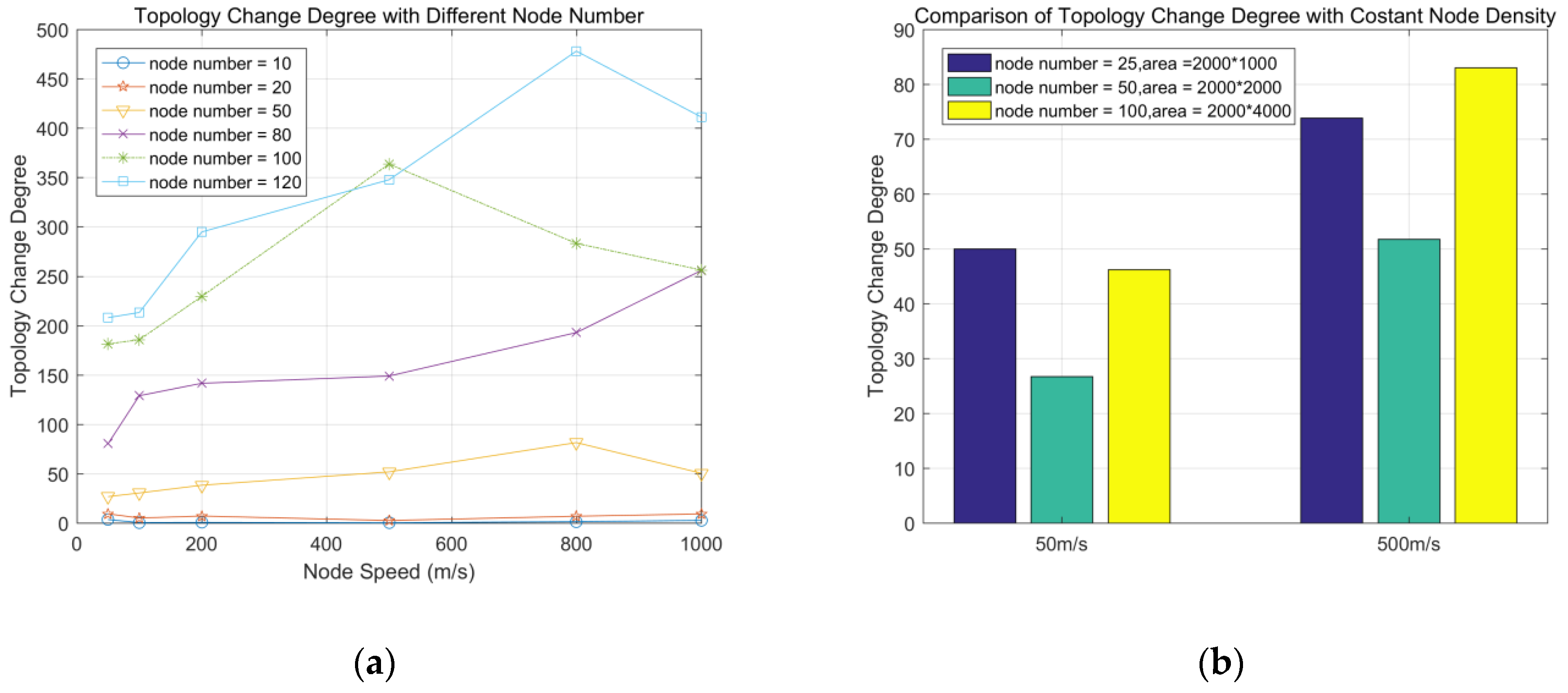
Case 1: The area of simulation region is fixed, and the number of nodes changes (the node density changes). We take the RWP model as an example. Figure 12a shows the result. It can be seen that in the same area of region, the value TCDntwrk increases as the density of nodes increases. This phenomenon can be explained by Equation (2). As the node density increases, the number of node neighbors also increases.
Case 2: The region is proportional to the number of nodes (the node density is constant). Here is also an example of RWP model. In Figure 12b, the node density is fixed to 0.000125. It shows that when the node density is constant, the change in TCD is not so large.
The value of TCD reflects the degree of topology change between nodes in the network. In fact, it also reflects the degree of aggregation of nodes and the degree of unified action between nodes.
It can be seen from Equations (1) to (3) that:
- For TCDi,j, the factors that affect its value include changes in velocity, direction, and distance between nodes.
- For TCDi,nbrs, in addition to each single TCDi,j value, the number of neighbor nodes within one hop is also one of the influencing factors.
- For TCDntwrk, the number of nodes in the network directly affects the value of TCDntwrk.
4.5. Disccusions
The TARCS routing scheme proposed in this paper is more suitable for complex scenarios with highly dynamic changes in network topology. The advantages are:
- Node cognition of its surroundings. Moving nodes can sense the topology environment between itself and neighboring nodes accurately and in a timely manner, thereby improving the node’s cognitive ability in regards to its environment.
- Adaptability. Nodes can adjust the routing protocol in real time according to the perceived result, and the adaptability of network is stronger.
- Scalability. The TARCS adaptive routing mechanism enables a FANET to adapt to changing scenarios. By modifying the topology change degree reference threshold/interval and adding alternate routing protocols, the TARCS can be extended to more scenarios and is compatible with more routing protocols.
In addition, the TARCS routing scheme proposed in this paper also proposes a new processing idea to deal with a highly dynamic MANET, namely, the topology-change-driven protocol selection framework. Compared with the proactive, reactive and hybrid routing protocols, TARCS is more adaptable. The specific description is shown in Table 5.
5. Conclusions
On the basis of analyzing the factors affecting the topology changes between nodes in FANETs, a mobility metric named topology change degree (TCD) is first proposed to describe the topology changes of highly dynamic FANETs. Meanwhile, a topology change awareness method is applied to measure topology changes by periodically sensing the topology changes of FANETs and to distinguish the mobility modes of nodes. Then a heuristic routing protocol scheme, TARCS, is proposed in this paper. The TARCS strategy is based on the periodic topology change sensing method, and adaptively selects appropriate routing protocols according to the comparison results of the measured topology change degree and the topology change degree threshold.
Different from the other single routing protocols proposed in other papers, the TARCS proposed in this paper is an adaptive routing strategy. It is based on the topology change perception between nodes and adaptively selects the routing protocol based on the perceived result. Essentially, it is a flexible routing protocol usage framework. Theoretical analysis and experiments show that:
- The topology change perception method can sense the topology changes of the network and distinguish several common mobility models of FANET.
- The combined use of routing protocols is more flexible and adaptable than using a single routing protocol in complex scenarios.
- Proper use of the TARCS scheme in complex scenarios can improve network performance.
Like mobile awareness, topology change perception opens the door to coping with and addressing the problems of highly dynamic FANETs topology changes. As an adaptive routing protocol framework, TARCS is only one of the applications of topology change perception and it proposes a routing implementation idea in a complex scenario of a FANET network. However, all of the above are just a preliminary framework, and there are a series of issues that need to be discussed and resolved. For example, how to effectively set the topology change perception interval? How to accurately calculate the topology change threshold? How to configure the weight factors among the influencing factors? How to deal with the problems of changes in the number of nodes? Subsequent work will continue to study in depth on the above issues.
Author Contributions
D.Z. is the project administrator. J.H. made the investigation. J.H. and D.Z. proposed the methodology. J.H. did the validation work and finished the original draft writing. D.Z. finished the review & editing writing.
Funding
This research received no external funding.
Conflicts of Interest
The authors declare no conflict of interest.
References
- Guillen-Perez, A.; Cano, M.D. Flying Ad Hoc Network: A New Domain for Network Communications. Sensors 2018, 18, 3571. [Google Scholar] [CrossRef] [PubMed]
- Bekmezci, İ.; Sahingoz, O.K.; Temel, Ş. Flying Ad-Hoc Networks (FANETs): A survey. Ad Hoc Netw. 2013, 11, 1254–1270. [Google Scholar] [CrossRef]
- Oubbati, O.M.; Lakas, A.; Zhou, F.; Güneş, M.; Yagoubi, M.B. A survey on position-based routing protocols for Flying Ad hoc Networks (FANETs). Veh. Commun. 2017, 10, 29–56. [Google Scholar] [CrossRef]
- Sarkar, S.K.; Basavaraju, T.G.; Puttamadappa, C. Routing Protocols. In Ad Hoc Mobile Wireless Networks-Principles, Protocols, and Applications, 2nd ed.; CRC Press: Boca Raton, FL, USA, 2012; pp. 81–126. [Google Scholar]
- Clausen, T.; Jacquet, P. Optimized Link State Routing Protocol (OLSR), RFC 3626 (Experimental). Available online: https://www.ietf.org/rfc/rfc3626.txt.pdf (accessed on 9 October 2018).
- Perkins, C.E.; Bhagwat, P. Highly Dynamic Destination-Sequenced Distance-Vector Routing (DSDV) for Mobile Computers. In Proceedings of the conference on Communications architectures, protocols and applications (SIGCOMM94), London, UK, 31 August–2 September 1994; pp. 234–244. [Google Scholar]
- Radhika Ranjan, R. Random Waypoint Mobility, Reference Point Group Mobility. In Handbook of Mobile Ad Hoc Networks for Mobility Models; Springer: Boston, MA, USA, 2011; pp. 637–670. [Google Scholar]
- Fan, B.; Sadagopan, N.; Helmy, A. The Important Framework for Analyzing the Impact of Mobility on Performance of Routing Protocols for Adhoc Networks. Ad Hoc Netw. 2003, 1, 383–403. [Google Scholar] [CrossRef]
- Hong, J.; Zhang, D. Impact Analysis of Node Motion on the performance of FANET routing protocols. In Proceedings of the 14th International Conference on Wireless Communications, Networking and Mobile Computing (WiCom2018), Chongqing, China, 18–20 September 2018. [Google Scholar]
- Sakhaee, E.; Jamalippour, A.; Kato, N. Aeronautical Ad Hoc Networks. In Proceedings of the IEEE Wireless Communications and Networking Conference (WCNC 2006), Las Vegas, NV, USA, 3–6 April 2006; pp. 246–251. [Google Scholar] [CrossRef]
- Zheng, Y.; Wang, Y.; Li, Z.; Dong, L.; Jiang, Y.; Zhang, H. A Mobility and Load aware OLSR routing protocol for UAV mobile ad-hoc networks. In Proceedings of the 2014 International Conference on Information and Communications Technologies (ICT2014), Nanjing, China, 15–17 May 2014. [Google Scholar]
- Zhou, J.H.; Lei, L.; Liu, W.K.; Tian, J. A simulation analysis of nodes mobility and traffic load aware routing strategy in aeronautical ad hoc networks. In Proceedings of the 2012 9th International Bhurban Conference on Applied Sciences & Technology (IBCAST), Islamabad, Pakistan, 9–12 January 2012; pp. 423–426. [Google Scholar]
- Hung, C.-C.; Chan, H.; Wu, E. Mobility Pattern Aware Routing for Heterogeneous Vehicular Networks. In Proceedings of the 2008 IEEE Wireless Communications and Networking Conference (WCNC2008), Las Vegas, NV, USA, 31 March–3 April 2008. [Google Scholar]
- Bamis, A.; Boukerche, A.; Chatzigiannakis, I.; Nikoletseas, S. A mobility aware protocol synthesis for efficient routing in ad hoc mobile networks. Comput. Netw. 2008, 52, 130–154. [Google Scholar] [CrossRef]
- Yu, Y.; Ru, L.; Chi, W.; Liu, Y.; Yu, Q.; Fang, K. Ant colony optimization based polymorphism-aware routing algorithm for ad hoc UAV network. Multimed. Tools Appl. 2016, 75, 14451–14476. [Google Scholar] [CrossRef]
- Swidana, A.; Abdelghanya, H.; Saifana, R.; Zilic, Z. Mobility and Direction Aware Ad-hoc on Demand Distance Vector Routing Protocol. Procedia Comput. Sci. 2016, 94, 49–56. [Google Scholar] [CrossRef] [Green Version]
- Khalaf, M.; Al-Dubai, Y.; Min, G. New efficient velocity-aware probabilistic route discovery schemes for high mobility Ad hoc networks. J. Comput. Syst. Sci. 2015, 81, 97–109. [Google Scholar] [CrossRef]
- Perkins, C.E.; Royer, E.M. Ad-hoc on-demand distance vector routing. In Proceedings of the Second IEEE Workshop on Mobile Computing Systems and Applications, New Orleans, LA, USA, 25–26 February 1999. [Google Scholar]
- Moussaoui, A.; Semchedine, F.; Boukerram, A. A link QoS routing protocol based on link stability for mobile ad hoc network. J. Netw. Comput. Appl. 2014, 39, 117–125. [Google Scholar] [CrossRef]
- Brahmbhatt, S.; Kulshrestha, A.; Singal, G. SSLSM: Signal Strength Based Link Stability Estimation in MANETs. In Proceedings of the 2015 International Conference on Computational Intelligence and Communication Networks, Jabalpur, India, 12–14 December 2015. [Google Scholar]
- Hong, X.; Gerla, M.; Pei, G.; Chiang, C.-C. A Group Mobility Model for Ad Hoc Wireless Networks. In Proceedings of the 2nd ACM international workshop on modeling, analysis and simulation of wireless and mobile systems, Seattle, WA, USA, 20 August 1999; pp. 53–60. [Google Scholar]
- Bonnmotion-A Mobility Scenario Generation and Analysis Tool. Available online: http://sys.cs.uos.de/bonnmotion/ (accessed on 10 October 2018).
- NS-3 Documentation. Available online: https://www.nsnam.org (accessed on 10 October 2018).
- Friis, H.T. A Note on a Simple Transmission Formula. Proc. IRE 1946, 34, 254–256. [Google Scholar] [CrossRef]
Figure 1.
MANET, VANET and FANET.
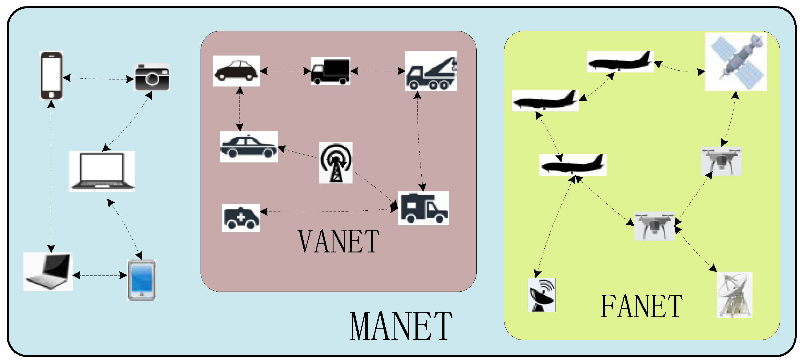
Figure 2.
The mobility aware methods and the subsequent processing methods.
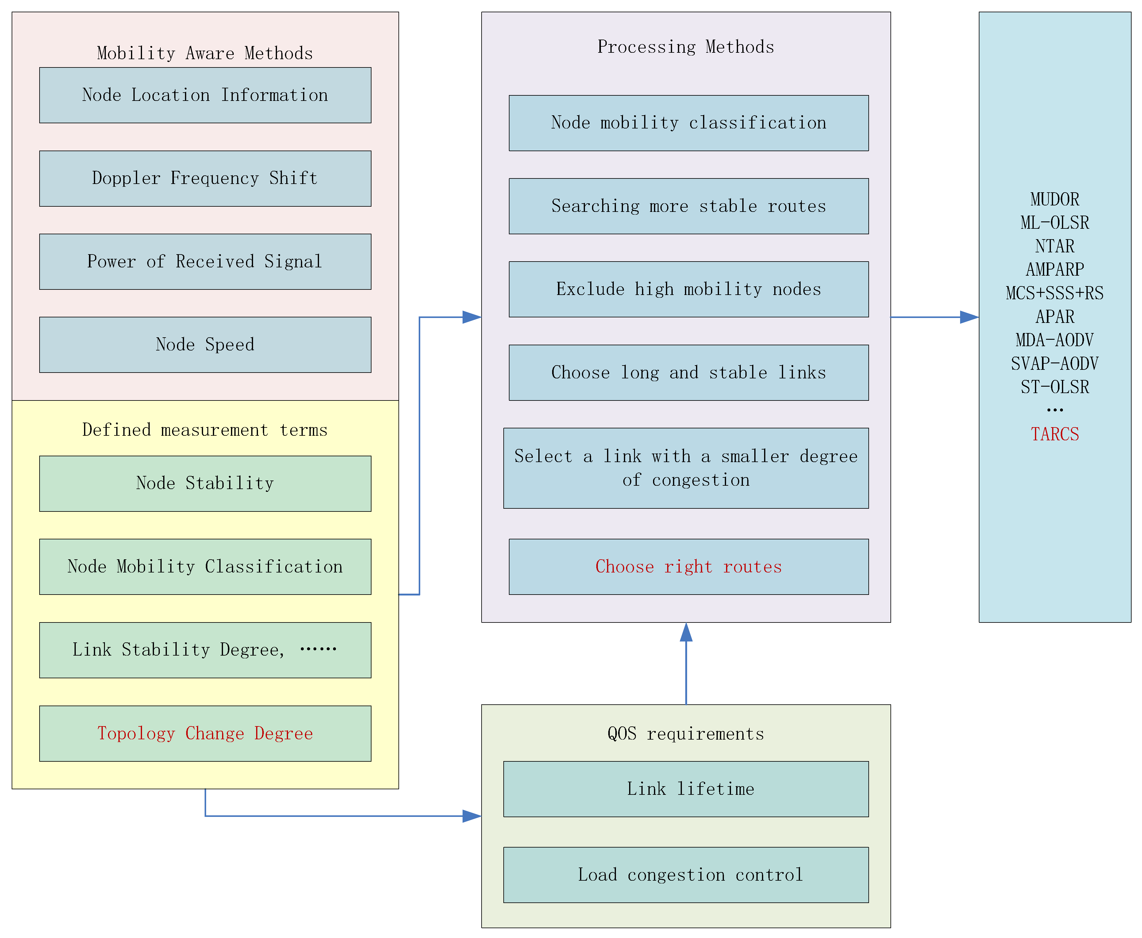
Figure 3.
Communication mode comparison between two nodes without and with the topology change aware routing protocol choosing scheme (TARCS). (a) Traditional communication mode between nodes without the TARCS; (b) communication mode between nodes with the TARCS.
Figure 3.
Communication mode comparison between two nodes without and with the topology change aware routing protocol choosing scheme (TARCS). (a) Traditional communication mode between nodes without the TARCS; (b) communication mode between nodes with the TARCS.
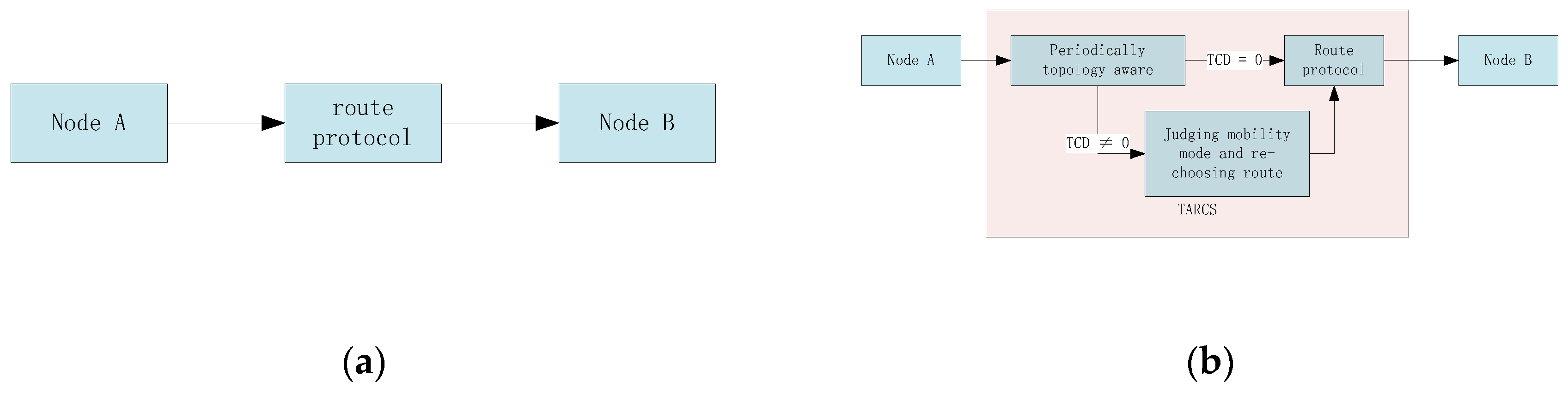
Figure 4.
Process flow of the TARCS.
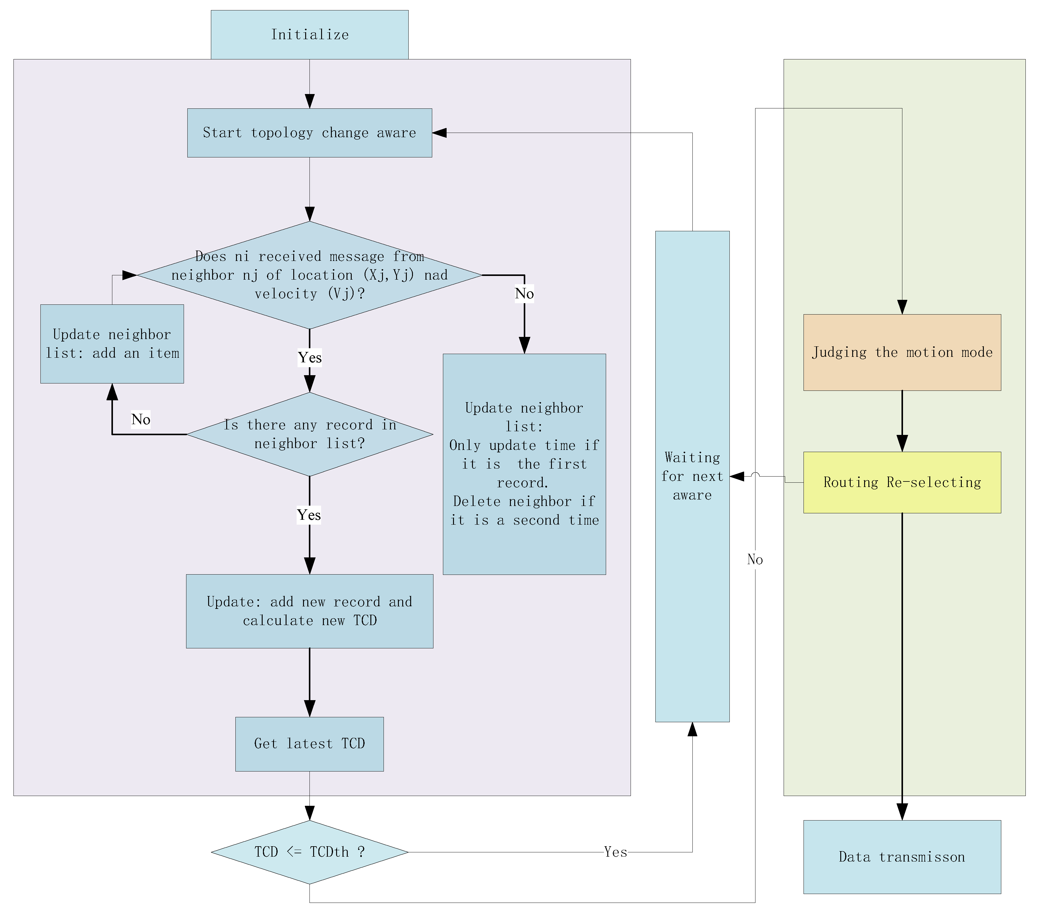
Figure 5.
Topology change caused by nodes distance change: (a) topology in the initial state; (b) topology after period T.
Figure 5.
Topology change caused by nodes distance change: (a) topology in the initial state; (b) topology after period T.
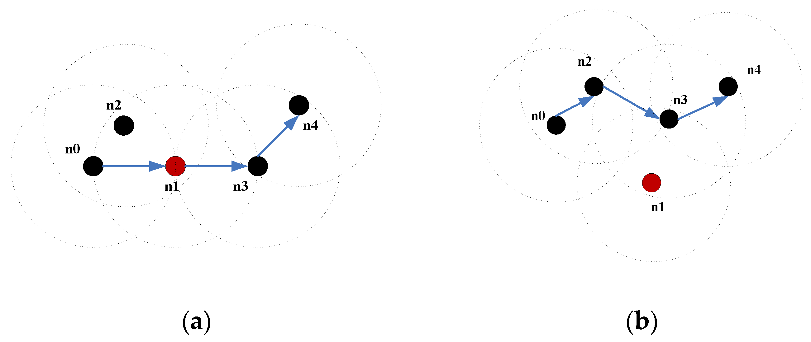
Figure 6.
Topology change caused by nodes direction change: (a) topology in the initial state; (b) topology after time T.
Figure 6.
Topology change caused by nodes direction change: (a) topology in the initial state; (b) topology after time T.
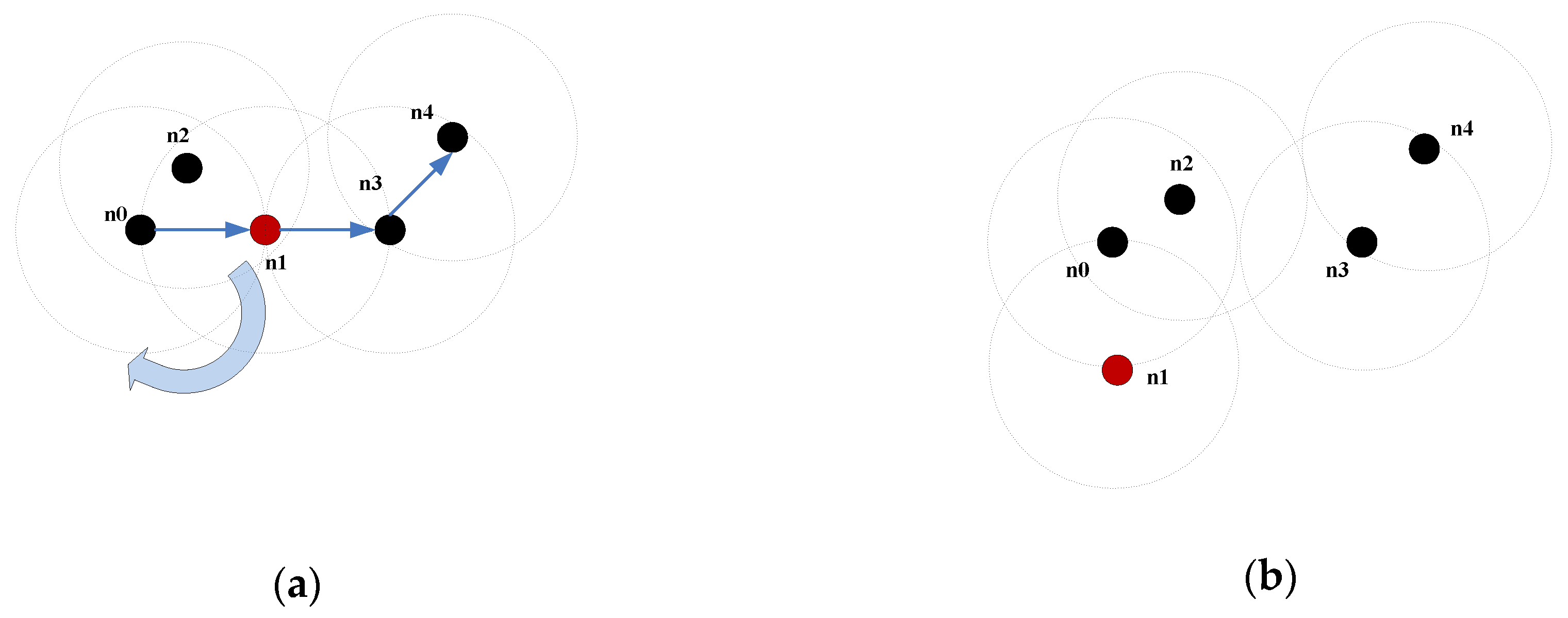
Figure 7.
Topology change caused by a difference of rate: (a) topology in the initial state; (b) topology after T time.
Figure 7.
Topology change caused by a difference of rate: (a) topology in the initial state; (b) topology after T time.
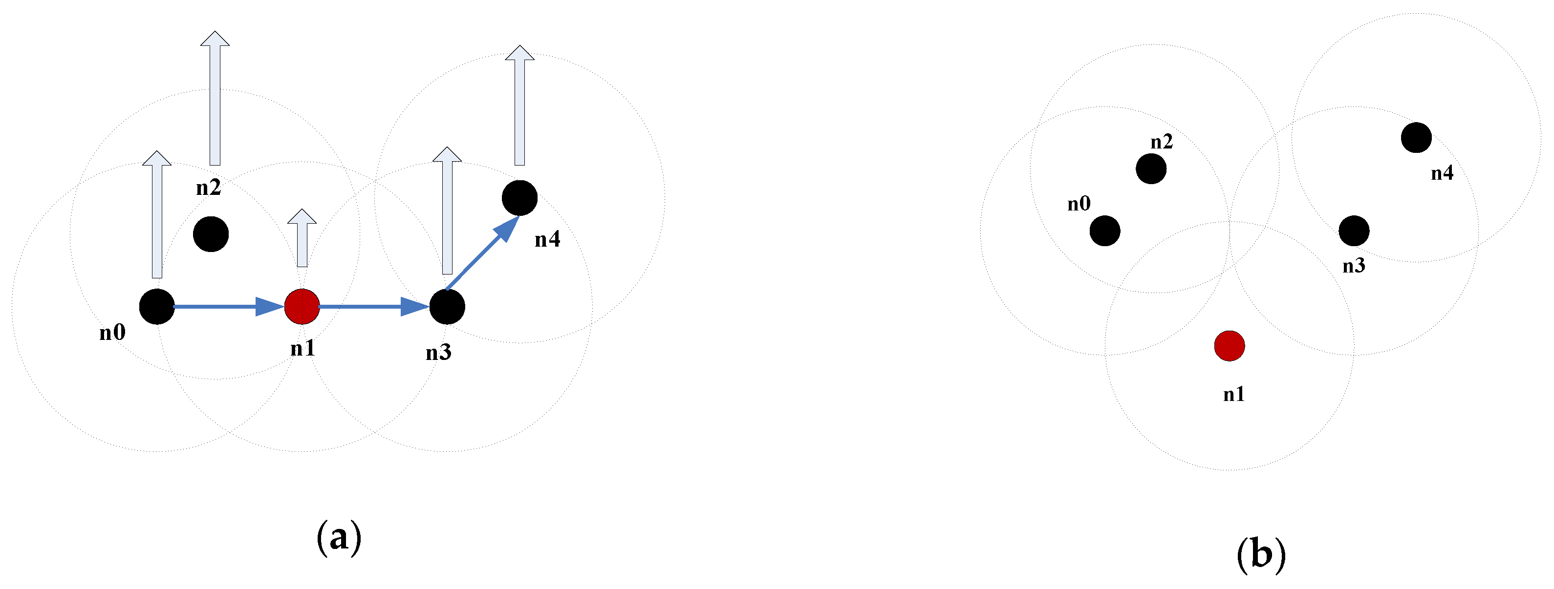
Figure 8.
Topology change caused by a change in the number of neighbors: (a) topology in the initial state; (b) topology after time T.
Figure 8.
Topology change caused by a change in the number of neighbors: (a) topology in the initial state; (b) topology after time T.
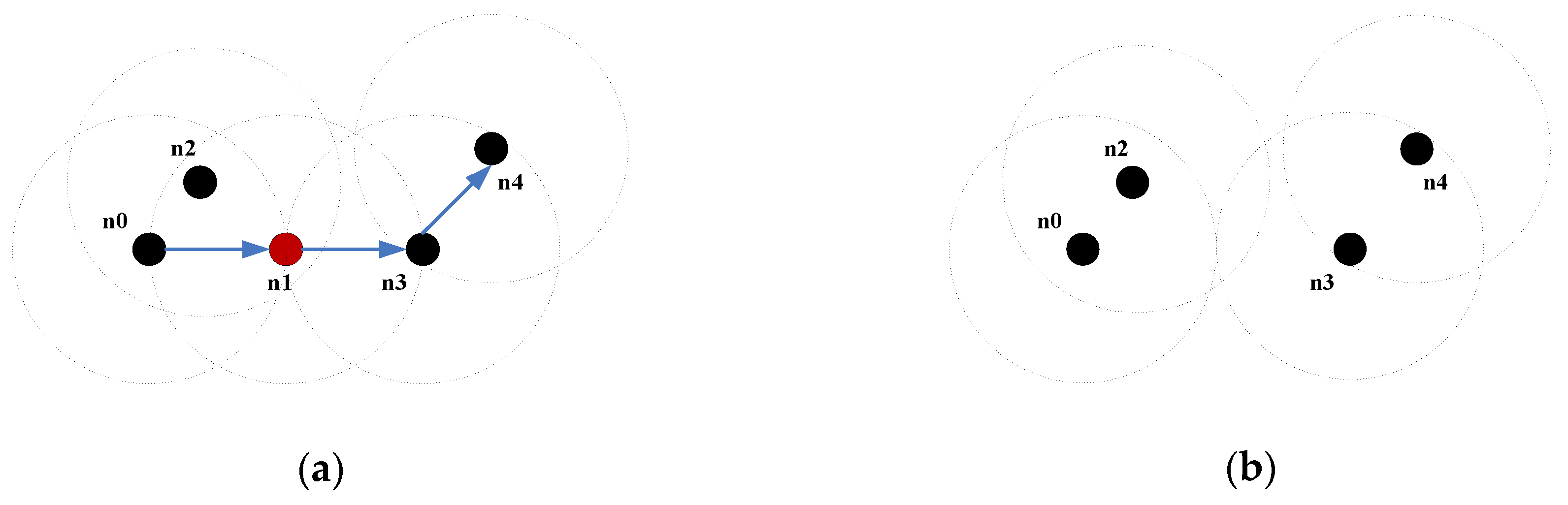
Figure 9.
Performance comparisons with and without the TARCS: (a) packet delivery ratio; (b) network throughput; (c) average end-to-end delay; (d) average jitter.
Figure 9.
Performance comparisons with and without the TARCS: (a) packet delivery ratio; (b) network throughput; (c) average end-to-end delay; (d) average jitter.

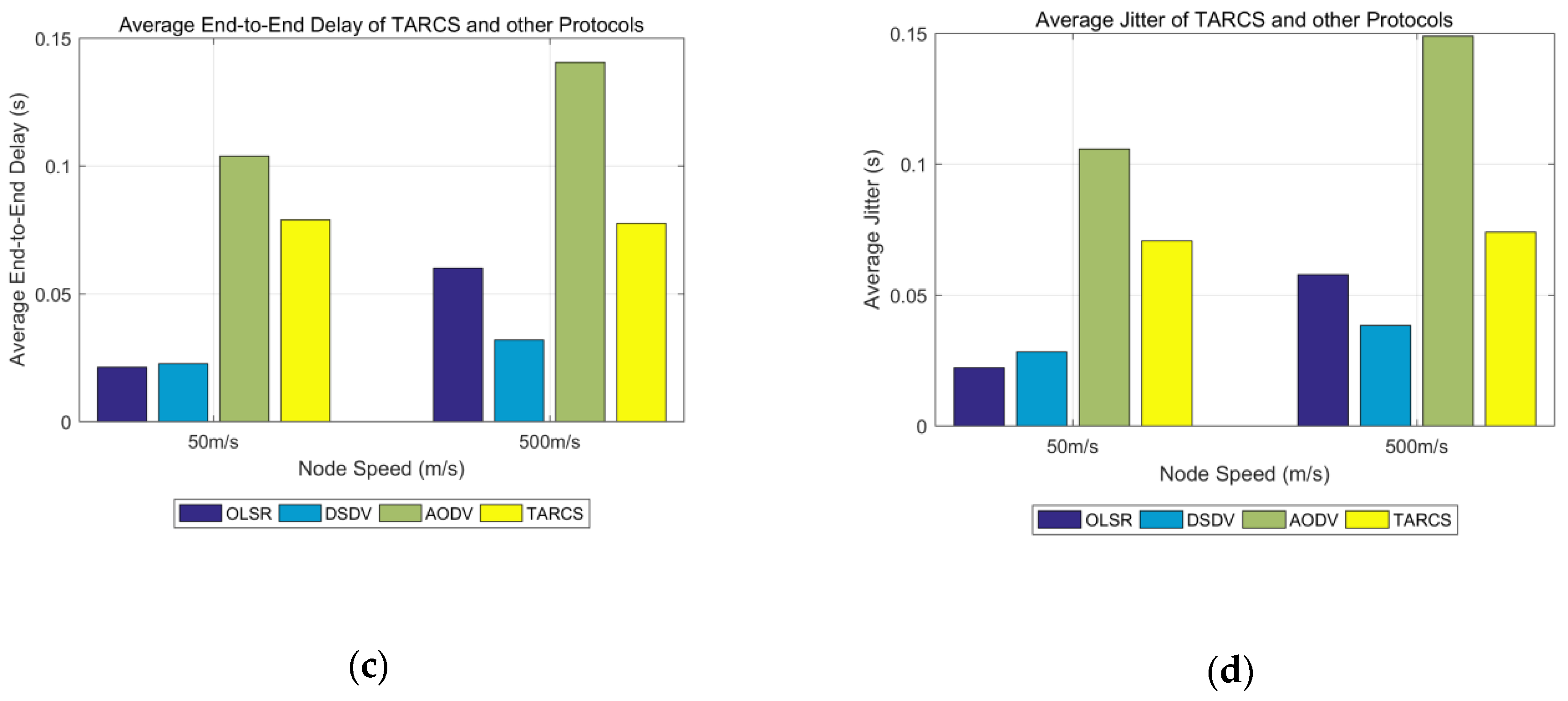
Figure 10.
Performance comparisons of different TARCS: (a) packet delivery ratio; (b) network throughput; (c) average end-to-end delay; (d) average jitter.
Figure 10.
Performance comparisons of different TARCS: (a) packet delivery ratio; (b) network throughput; (c) average end-to-end delay; (d) average jitter.
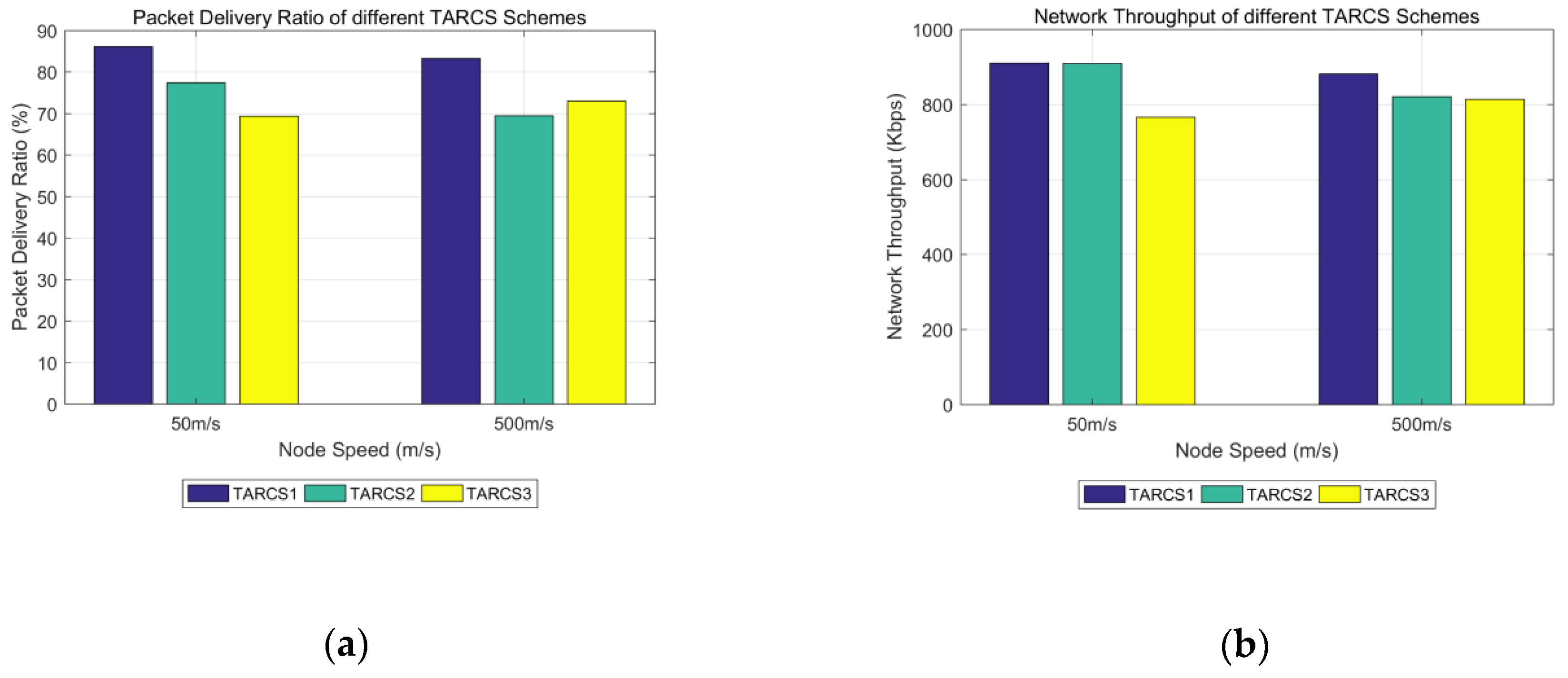

Figure 11.
Comparisons of topology change degree values with different mobility patterns: (a) TCDntwrk; (b) the average of TCDntwrk (1-RWP, 2-RPGM (g = 50), 3-RPGM (g = 25), 4-RPGM (g = 10), 5-RPGM (g = 5), 6-Pursue).
Figure 11.
Comparisons of topology change degree values with different mobility patterns: (a) TCDntwrk; (b) the average of TCDntwrk (1-RWP, 2-RPGM (g = 50), 3-RPGM (g = 25), 4-RPGM (g = 10), 5-RPGM (g = 5), 6-Pursue).

Figure 12.
Comparisons of TCDntwrk with changed node density and fixed node density: (a) the node density is variable; (b) the node density is fixed.
Figure 12.
Comparisons of TCDntwrk with changed node density and fixed node density: (a) the node density is variable; (b) the node density is fixed.

Table 1.
Comparison of MANET, VANET and FANET.
| Characteristics | MANET | VANET | FANET | |||
|---|---|---|---|---|---|---|
| Small UAVs | Large UAVs | |||||
| FW * | RW * | FW * | RW * | |||
| Node Speed | Low | Medium | Medium | Medium | High | High |
| Density | High | High | Low | |||
| Power Consumption | Low | High | Med | Med | High | High |
| Network Connectivity | High | Medium | Low | |||
| QoS | Medium | Depends on the applications | ||||
| Mobility Patterns | 2D | 2D | 3D | |||
| Mobility Degree | Low | Medium | Low-Med | Low-Med | Med-High | Med-High |
| Altitude | Close to ground | Close to ground | Low | Low | High | High |
| Static Pause | Yes | Yes | No | Yes | No | Yes |
| Topology Variation | Occasionally | Frequently | Very frequently | Very frequently | ||
| scalability | Medium | High | Low | |||
| Typical Mobility Models | regular | Restricted through roads | Depends on the applications and need to pre-determined | |||
* FW: fixed-wing, * RW: rotary wing.
Table 2.
Parameters of simulation experiments.
| Parameters | Values |
|---|---|
| Simulation region | 2000 m × 2000 m |
| Node number | 50 |
| Mobility Model | Chain: RWP + RPGM (g = 5) + Pursue |
| Simulation Time | 602 s |
| Node speed | 50 m/s, 500 m/s |
| Route protocol | OLSR / AODV / DSDV |
| Propagation model | Free space propagation model |
| Delay model | constant speed propagation delay model |
| Data mode | CBR |
| Packet size | 1024 bytes |
| Data rate | 16 Kbps |
| MAC protocol | IEEE 802.11bDCF |
| Transmission range | 140 m |
Table 3.
The topological change degree (TCD) perception results and route protocol choosing scheme of Experiment 1.
Table 3.
The topological change degree (TCD) perception results and route protocol choosing scheme of Experiment 1.
| Perceptual Moment | Actual Mobility Model | Node Speed = 50 m/s | Node Speed = 500 m/s | Route Protocol | ||
|---|---|---|---|---|---|---|
| TCD(t) | Judged model | TCD(t) | Judged model | |||
| 0 | RWP | 0 | RWP | 0 | RWP | AODV |
| 50 | RWP | 2.078 | RWP | 0 | RWP | AODV |
| 100 | RWP | 15.459 | RWP | 842.592 | RWP | AODV |
| 150 | RWP | 34.364 | RWP | 782.536 | RWP | AODV |
| 200 | RPGM (g = 5) | 177.845 | RPGM | 589.106 | RWP | AODV |
| 250 | RPGM (g = 5) | 560.596 | RPGM | 2513.24 | Pursue | DSDV |
| 300 | RPGM (g = 5) | 658.254 | RPGM | 678.321 | RWP | AODV |
| 350 | RPGM (g = 5) | 493.418 | RPGM | 2102.88 | Pursue | DSDV |
| 400 | Pursue | 1963.96 | Pursue | 4144.1 | Pursue | DSDV |
| 450 | Pursue | 974.397 | RPGM | 2042.52 | Pursue | DSDV |
| 500 | Pursue | 3800.78 | Pursue | 2312.88 | Pursue | DSDV |
| 550 | Pursue | 2332.39 | Pursue | 4482.67 | Pursue | DSDV |
| 600 | Pursue | 4786.97 | Pursue | 3666.45 | Pursue | DSDV |
Table 4.
Three different schemes of TARCS.
| Mobility Model | TARCS1 | TARCS2 | TARCS3 |
|---|---|---|---|
| RWP | AODV | OLSR | AODV |
| RPGM (g = 5) | AODV | AODV | DSDV |
| Pursue | DSDV | DSDV | DSDV |
Table 5.
T Comparisons of topology-change-driven route and other route protocols.
| Types of Route Protocols | Characteristics | Advantages | Disadvantages |
|---|---|---|---|
| Proactive routing protocol | Periodically maintain routing links; suitable for small networks. | Short delay; high quality of service; long-pass link. | High energy consumption; heavy network load and high node congestion level. |
| Reactive routing protocol | Establish routing discovery when needed. | Low energy consumption; light routing load. | The pass-link is not guaranteed. It takes time to establish a link. Once the link is interrupted, it needs to be re-established. |
| Hybrid routing protocol | Combined with proactive and reactive routing. Suitable for hierarchical networks. | Using proactive routing within the cluster, reactive between clusters | Only suitable for hierarchical networks. |
| Topology-change-driven protocol | Reselect the appropriate route based on topology changes. | Nodes obtain information of the surrounding topology changes in time. Multiple routing protocols are used in combination to suit complex scenarios. | Dependent on reference threshold settings and specific routing strategies. |
© 2019 by the authors. Licensee MDPI, Basel, Switzerland. This article is an open access article distributed under the terms and conditions of the Creative Commons Attribution (CC BY) license (http://creativecommons.org/licenses/by/4.0/).
Share and Cite
MDPI and ACS Style
Hong, J.; Zhang, D. TARCS: A Topology Change Aware-Based Routing Protocol Choosing Scheme of FANETs. Electronics 2019, 8, 274. https://doi.org/10.3390/electronics8030274
AMA Style
Hong J, Zhang D. TARCS: A Topology Change Aware-Based Routing Protocol Choosing Scheme of FANETs. Electronics. 2019; 8(3):274. https://doi.org/10.3390/electronics8030274
Chicago/Turabian StyleHong, Jie, and Dehai Zhang. 2019. "TARCS: A Topology Change Aware-Based Routing Protocol Choosing Scheme of FANETs" Electronics 8, no. 3: 274. https://doi.org/10.3390/electronics8030274
Note that from the first issue of 2016, this journal uses article numbers instead of page numbers. See further details here.