Motion Planning of a Second-Order Nonholonomic Chained Form System Based on Holonomy Extraction


School of Information Science and Technology, Aichi Prefectural University, Nagakute, Aichi 480-1198, Japan
Electronics 2019, 8(11), 1337; https://doi.org/10.3390/electronics8111337
Submission received: 11 September 2019
/
Revised: 1 November 2019
/
Accepted: 5 November 2019
/
Published: 12 November 2019
(This article belongs to the Special Issue Motion Planning and Control for Robotics)
Abstract
:This paper proposes a motion planning algorithm for dynamic nonholonomic systems represented in a second-order chained form. The proposed approach focuses on the so-called holonomy resulting from a kind of motion that traverses a closed path in a reduced configuration space of the system. According to the author’s literature survey, control approaches that make explicit use of holonomy exist for kinematic nonholonomic systems but does not exist for dynamic nonholonomic systems. However, the second-order chained form system is controllable. Also, its structure analogizes with the one of the first-order chained form for kinematic nonholonomic systems. These survey and perspectives brought a hypothesis that there exists a specific control strategy for extracting holonomy of the second-order chained form system to the author. To verify this hypothesis, this paper shows that the holonomy of the second-order chained form system can be extracted by combining two appropriate pairs of sinusoidal inputs. Then, based on such holonomy extraction, a motion planning algorithm is constructed. Furthermore, the effectiveness is demonstrated through some simulations including an application to an underactuated manipulator.
1. Introduction
Nonholonomic systems—dynamical systems with non-integrable differential constraints—have attracted attention as challenging robotic systems in the fields of motion planning and control [1,2,3,4]. The most symbolical control problem is characterized by Brockett’s theorem [5]. It provides a well-known fact that nonholonomic systems cannot be stabilized by using pure smooth state feedback control. According to the kind of constraints, the nonholonomic systems are generally classified into two types: kinematic ones and dynamic ones. The former, which are subject to velocity constraints, include a wheeled mobile robot without or with trailers [1], a snakeboard [1] and a trident snake robot [6]; the latter, which are subject to acceleration constraints, include an underactuated manipulator [7,8,9,10], a surface vessel [11,12], and a blimp [13].
Nonholonomic systems have an intrinsic property that a part of states is impossible to change by an individual control input. The key to control such states is to combine the effects of multiple control inputs in order to extract a kind of motion expressed by Lie brackets. For a class of kinematic nonholonomic systems, holonomy (or geometric phase) is defined as “the extent to which a closed path in the base space fails to be closed in the configuration space” [14], where the base space is a reduced configuration space. The effect which corresponds to Lie brackets is generated by periodic control inputs. It can be said as the essential motion of kinematic nonholonomic systems. In fact, several control approaches utilize the holonomy [1,14,15,16,17,18,19,20].
Table 1 summarizes main control approaches proposed so far for nonholonomic systems. The control approaches are classified into three groups by the type of constraints and also, in each group, sorted by the published year. From Table 1, the following points can be seen:
- As a canonical form for nonholonomic systems, the chained form is often used over all kinds of constraints.
- Many studies have been attracted to a feedback control problem related Brockett’s theorem independently of the type of constraints.
- For kinematic nonholonomic systems, there are some control approaches that explicitly use holonomy especially in motion planning; for dynamic or third-order nonholonomic systems, there is no such control approach.
On the other hand, by comparing the first- and second-order chained form systems, it can be found that the structures are similar unless the number of integrators is different. This perspective and the above-mentioned survey led the author to a hypothesis that there exists an appropriate pair of sinusoids to extract holonomy of the second-order chained form system.
Motivated by the hypothesis, this paper addresses a motion planning problem for the second-order chained form system. A class of dynamic nonholonomic systems can be represented as the second-order chained form by transforming the generalized coordinates and control inputs appropriately [8,9,12]. The second-order chained form system is described as a type of affine systems which is nonlinear controllable. Inspired by the structural difference and analogy between the first- and second-order chained form systems, it is found that a combination of two appropriate pairs of sinusoidal inputs can be used to extract the holonomy. This verifies the hypothesis. The idea of holonomy extraction is available directly to motion planning. The proposed motion planning algorithm can be applied to an underactuated manipulator. Its effectiveness is demonstrated by some simulation results.
The main contributions of the proposed approach are emphasized as follows:
- A specific way to extract holonomy of the second-order chained form system was proposed. Based on holonomy extraction, a motion planning algorithm was constructed.
- The holonomy-based motion planning algorithm was applied to an underactuated manipulator. The usefulness of the proposed algorithm was validated through some simulation results.
- To the best of the author’s knowledge, no control approach that makes explicit use of the holonomy for the second-order chained form system has been previously reported as shown in Table 1.
This paper has improved the preliminary results of the author’s previous studies [33,34]. In Reference [33], the author has first proposed a specific strategy of holonomy extraction for the second-order chained form system. In addition to that, this paper presents another strategy (see Remark 1). The holonomy obtained in each strategy was also visualized in some phase spaces to understand the differences (see Figures 2 and 4). In Reference [34], the author has applied the holonomy-based motion planning algorithm into an underactuated manipulator and discussed singularities of the system transformation therein. Instead of such discussion, this paper examine an effect from the parameters of control inputs (see the second last paragraph in Section 4, that is, the paragraph before Remark 5).
The rest of the paper is organized as follows. In Section 2, a system representation of the second-order chained form system is given and then its controllability is confirmed. In Section 3, to extract the holonomy of the system, appropriate pairs of sinusoids is concretely provided; based on the maneuver of holonomy extraction, a motion planning algorithm is also proposed. In Section 4, the algorithm is applied to an underactuated manipulator. In the last section, the paper is concluded with directions for future work.
2. Second-Order Nonholonomic Chained Form System and Its Controllability
Consider the following second-order chained form system:
which is one canonical representation for a class of dynamic nonholonomic systems. This system can be obtained from the original dynamical model via an appropriate transformation of the generalized coordinates and control inputs. By defining a state vector by , in state space form, (1) is represented as an affine nonlinear system
where
Note that the system (2) has equilibrium points at with .
According to Sussmann’s theorem [35], the small-time local controllability (STLC) of the affine system (2) is easily confirmed. For a Lie bracket , let , and be defined as the number of times that , and occur in , respectively. If is odd and is even for each , the bracket is called “bad”; otherwise, the bracket is called “good”. Also, let be defined as the degree of . Then, in the Philip Hall bases [1] of (2), the non-zero vector fields at are as follows:
Six appropriate vector fields out of (6)–(13) can span , which means that the system is locally accessible. In other words, the so-called Lie Algebra Rank Condition (LARC) is satisfied. On the other hand, all bad brackets , , and , are zero vector fields at . This obviously can be expressed by linear combinations of good brackets of lower degree Thus the second-order chained form system (1) is small-time local controllable at .
From the above-mentioned controllability analysis, there exists an admissible control input such that the system can be steered from any equilibrium point to its neighborhood for a small time. This, however, does not imply that a specific control input is obtained. As a specific solution, the subsequent section presents a motion planning algorithm that makes use of holonomy extraction.
3. Motion Planning Based on Holonomy Extraction
This section considers a motion planning problem of the second-order chained form system and presents an algorithm to solve it. The key idea is to extract holonomy of the system by using sinusoidal inputs. Based on that, the proposed algorithm can be simply constructed.
3.1. Problem Formulation
The following motion planning problem is addressed in this paper:
Problem 1.
The affine system (2) can be divided into two parts: the double-integrator part with respect to ; and the residual part with respect to . The former is linear controllable, so it is easy to control the four states. The latter nonlinear part is what we should focus on here. According to the controllability analysis in the last section, displacement of only requires the third-order Lie brackets such as (10) and (11); displacement of only requires the fourth-order Lie brackets such as (12) and (13). In general, however, handling higher-order Lie brackets is quite difficult [6].
3.2. Holonomy Extraction by Using Sinusoidal Inputs
For the difficulty to obtain displacement of and , this subsection presents how to break it through by using sinusoidal inputs.
What we should do for verifying the hypothesis presented in Section 1 is to find an appropriate pair of sinusoids such that displacement of and is obtained as holonomy—a kind of motion that traverses a closed path in a reduced configuration space of . Note that the motion planning problem we address is based on the equilibrium points, that is, . So, the desired holonomy is the one to excite to be a certain value and to be zero.
Now consider two control inputs of zero-mean sinusoidal functions with angular frequency , that is, period and amplitude , , where a and b are positive constants. The time span for applying control inputs is also assumed to be composed of two periods: and . By direct calculation, we analyze how the system is steered by a pair of given sinusoidal inputs over each period. First, let the initial equilibrium point be , and let the pair of control inputs over the first period be
Then, the trajectories of and their time derivatives become
Consequently, the values at are
From (18), the trajectories of and its time derivative are given by
Hence, we obtain the values of and at as follows:
At this moment, each non-zero displacement from the initial value is expressed as and in (20) and (26), respectively. As one of a pair of control inputs such that , and at , we choose the following pair of sinusoidal functions over the second period :
Note that (27) is the sign inversion of (14). By using (19)–(22), the trajectories of and their time derivatives can be written as
Their values at are also computed as
Since the trajectory of behaves according to (31), and over can be expressed by
Finally, from (36) and (37), the reaching values at are provided as
Therefore, the results (32)–(35), (38) and (39) mean that combining two pairs of sinusoidal inputs (14) and (27), that is,
provides the desired holonomy. This verified the hypothesis. Although this approach is heuristic and constructive, it brings the obvious relationship between parameters of the inputs and the magnitude of the holonomy. In fact, the displacement of at , that is, with the parameters: a and b; the displacement of at , that is, the state, depends on not only a and b but also .
Figure 1 shows the control inputs with , the resultant velocities and positions. Also, Figure 2 depicts the trajectories in various phase spaces. Trajectories of velocities and positions were (not analytically but) numerically obtained. The simulator was developed in C with the GNU Scientific Library [36]. The embedded eight-th order Runge-Kutta Prince-Dormand method with nine-th order error estimate (rk8pd) was selected as an ODE solver, where an absolute and relative errors were set to and 0, respectively.
From Figure 1b,c, it can be observed that a positive displacement with respect to is obtained by two-period motion. Since in (39), the magnitude of the holonomy is computed as . Figure 2 shows the holonomy in six different types of phase spaces, which visualizes that the displacement of results from a kind of motion that traverses a closed path in a reduced configuration space of . In particular, Figure 2b,f present that the motion to extract the holonomy is characterized by two closed circular paths in the reduced configuration space.
In fact, it is verified that the same displacement as in (39) is obtained by combining two pairs of sinusoidal inputs (14) and (27) in the reverse order of (40), that is,
Let us synthesize (40) and (41) as follows:
Also, we can easily confirm that the following pairs of control inputs other than (42) yield a positive displacement of :
Moreover, two appropriate pairs of sinusoidal inputs such that a negative displacement with respect to can be obtained include the following forms:
Remark 1.
The common strategy among (42)–(45) is, in the second period, to keep while canceling or arisen over the first period. To accomplish it, (42)–(45) in the second period make use of the sinusoidal inputs which are the sign inversion of those over the first period. Alternatively, we can employ a fact that and are not driven by only either or . For example, if we adopt
instead of (27), then . Note that the magnitude of the holonomy resulted from a pair of (14) and (46) is half of the one resulted from a pair of (14) and (27). The control inputs and the resultant states with are shown in Figure 3. Then, the magnitude of the holonomy is computed as . Figure 4 visualizes the holonomy of this case in six different types of phase spaces. By contrast with Figure 2b,f, it can be seen that the holonomy in Figure 4b,f is extracted by traversing one closed circular path in the reduced configuration space. The alternative way such as (46) is applicable not only to (42) but also to (43)–(45) as follows:
3.3. Holonomy-Based Motion Planning Algorithm
Based on the holonomy extraction of the previous subsection, a motion planning algorithm can be easily constructed.
Here, let us assume the following points:
- The entire motion planning consists of three phases: , and . Also, the periods of and are T, whereas that of is .
- At the beginning and end of each phase, the system (1) stops; that is to say, each velocity is zero.
- Let , , be an appropriate sinusoidal function whose period is T.
The basic algorithm of motion planning to steer from an equilibrium point to the other equilibrium point is as follows (see Figure 5 as the corresponding flowchart):
- Step 1:
- Set the initial state of the system, that is, .
- Step 2:
- In , steer only from to by using .
- Step 3:
- In , steer only from to by using .
- Step 4:
Note that Steps 1–3 are replaceable.
Now let us consider an example of motion planning from an initial state to a desired state for four seconds (i.e., ). As control inputs such that the control objective is achieved, we adopt
The system starts to move from the initial state at , through
at and
at and lastly reaches the following final states:
Therefore, the results (60)–(62) indicate the following things:
- to realize , and must be
- to realize , and should be assigned as, for example,
Figure 6 depicts the control inputs with (64) and (65), the resultant velocities and positions. From Figure 6b,c, it can be confirmed that the state arrives at , that is, the desired motion is successfully planned.
Remark 2.
The control inputs with (64) and (65) have switching points between and , between and and in the middle of . The corresponding effect cannot be found in the resultant velocities and positions. In a practical situation, however, a combination with feedback control should be required to compensate the occurred error. This is included in future work.
Remark 3.
Note that there exists freedom to choose and . The freedom can be utilized for designing the motion of the system. Under the above-mentioned control objective, you can choose and such that . Its example of use will be shown in the next section.
4. Application to Rest-to-Rest Motion of a Three-Joint Manipulator with Passive Third Joint
This section applies the proposed algorithm into a rest-to-rest motion of an underactuated planar manipulator that moves in a horizontal plane. The manipulator has three joints whose third joint is passive (i.e., unactuated) as depicted in Figure 7.
The main variables and parameters are defined as in Table 2.
For simplicity, assume that there is no external disturbance such as load, friction, linear and nonlinear damping acting on each joint. Then, based on Lagrange’s equation of motion, the dynamics of the manipulator is given by
where and are vectors of joint angles and torques, respectively. Note that (66) does not include the gravitational term because the dynamics is not affected from gravitational forces. See Appendix A for the details of the inertia matrix and the centrifugal and Coriolis term .
Yoshikawa, et al. [9] considered the same case, and also gave a set of coordinate and input transformation that can transform system (66) to
where and . In addition, using the coordinate transformation
where and the input transformation
can transform system (67) to the second-order chained form system (1) [9]. Note that both transformation are singular at .
We here suppose a motion from to that is subject to . The correspondence between (67) and (1) implies that the system (67) with the input transformation (69) can be controlled by the motion planning algorithm presented in Section 3.3. Then, a control procedure for achieving such motion is as follows (see Figure 8 as the corresponding diagram):
- Step 1:
- For a given initial position and a desired position , compute their corresponding positions and by using (68).
- Step 2:
- Plan motion so as to steer the system (1) from to by using the holonomy-based motion planning algorithm presented in the last section. As a result, the corresponding sinusoidal inputs is obtained.
- Step 3:
Remark 4.
Let us consider that a three-joint underactuated manipulator with , , , , that is, conducts a rest-to-rest motion from to . Then, and correspond to and , respectively. The following set of control inputs to (1) can be applied:
with and such that holds.
Simulations were performed for three kinds of : , and . As the simulation results, Figure 9, Figure 10 and Figure 11 show positions, velocities, and control inputs of (67). From Figure 9, the following facts can be observed:
- the desired rest-to-rest motion on is achieved;
- If is greater than , then, on the basis of the case when , becomes bigger and becomes smaller; that is to say, the third link moves broadly in direction of x-axis while its orientation varies slightly smaller.
- If is less than , then, on the basis of the case when , becomes smaller and becomes bigger; that is to say, the third link moves narrowly in direction of x-axis while its orientation varies slightly larger.
The last two facts indicate that the freedom in choosing and can be used for obstacle avoidance. If there is an obstacle in the gray-hatched area of Figure 11, choosing and such that is less than can make the third link avoid colliding to the obstacle. Therefore, the simulation results illustrated the effectiveness of the proposed algorithm.
5. Conclusions
In this paper, a holonomy-based motion planning algorithm for the second-order chained form system was proposed. First, it was shown that a combination of two appropriate pairs of sinusoidal inputs extracts the holonomy. This verified the hypothesis that motivated this study. Next, the idea of holonomy extraction was directly used to construct a motion planning algorithm. Finally, the effectiveness of the proposed algorithm was confirmed from the simulation results including an application to an underactuated manipulator.
This algorithm is heuristic but simple and useful. By adopting specific sinusoids as control inputs, the relationship between parameters of control inputs and the magnitude of the holonomy was revealed. Also, it was found that the freedom to choose the parameters can be utilized for designing the motion of the system. Accordingly, the proposed algorithm will provide a new perspective on how to control dynamic nonholonomic systems.
Future work will include experimental validation and generalization of the controlled systems and control inputs. In particular, a combination with feedback control should be needed in practice to make the proposed approach robust against the modeling error and external disturbance. Also, to enlarge applicable systems, an extension to an underactuated system under the gravity will be considered.
Funding
This work was supported by JSPS KAKENHI Grant Number 26820169.
Acknowledgments
The author would like to thank the anonymous reviewers for their insightful comments and suggestions.
Conflicts of Interest
The authors declare no conflict of interest.
Abbreviations
The following abbreviations are used in Table 1:
| AISMC | Adaptive Integral Sliding Mode Control |
| AUV | Autonomous Underwater Vehicle |
| BS | BackStepping |
| CF | Chained Form |
| EM | Equilibrium Manifold |
| FB | FeedBack |
| FL | Feedback Linearization/Linearized |
| IDA-PBC | Interconnection and Damping Assignment Passivity-Based Control |
| MP | Motion Planning |
| MPC | Model Predictive Control |
| UAM | UnderActuated Manipulator |
Appendix A. The Details of the Inertia Matrix and the Centrifugal and Coriolis Term in (66)
For the three-joint manipulator depicted in Figure 6, the inertia matrix and the centrifugal and Coriolis term are given as
where
References
- Murray, R.M.; Li, A.; Sastry, S.S. A Mathematical Introduction to Robotic Manipulation; CRC Press: Boca Raton, FL, USA, 1994; ISBN 978-0849379819. [Google Scholar]
- LaValle, S.M. Planning Algorithms; Cambridge University Press: New York, NY, USA, 2006; ISBN 978-0521862059. [Google Scholar]
- Liu, Y.; Yu, H. A survey of underactuated mechanical systems. IET Control Theory Appl. 2013, 7, 921–935. [Google Scholar] [CrossRef]
- Bloch, A.M. Nonholonomic Mechanics and Control, 2nd ed.; Interdisciplinary Applied Mathematics, 24, Krishnaprasad, P.S., Murray, R.M., Eds.; Springer-Verlag: New York, NY, USA, 2015; ISBN 978-1493930166. [Google Scholar]
- Brockett, R.W. Asymptotic stability and feedback stabilization. In Differential Geometric Control Theory; Brckett, R.W., Millmann, R.S., Sussmann, H.J., Eds.; Birkhauser Verlag: Basel, Switzerland, 1983; pp. 181–191. ISBN 978-0817630911. [Google Scholar]
- Ishikawa, M.; Minami, Y.; Sugie, T. Development and control experiment of the trident snake robot. IEEE/ASME Trans. Mechatron. 2010, 15, 9–16. [Google Scholar] [CrossRef]
- Oriolo, G.; Nakamura, Y. Free-joint manipulators: motion control under second-order nonholonomic constraints. In Proceedings of the IEEE/RSJ International Workshop on Intelligent Robots and Systems (IROS’91), Osaka, Japan, 3–5 November 1991; pp. 1248–1253. [Google Scholar] [CrossRef]
- Imura, J.; Kobayashi, K.; Yoshikawa, T. Nonholonomic control of 3 link planar manipulator with a free joint. In Proceedings of the 35th IEEE Conference on Decision and Control (CDC’96), Kobe, Japan, 13 December 1996; pp. 1435–1436. [Google Scholar] [CrossRef]
- Yoshikawa, T.; Kobayashi, K.; Watanabe, T. Design of a desirable trajectory and convergent control for 3-D. O.F manipulator with a nonholonomic constraint. In Proceedings of the 2000 IEEE International Conference on Robotics and Automation (ICRA’00), San Francisco, CA, USA, 24–28 April 2000; pp. 1805–1810. [Google Scholar] [CrossRef]
- Arai, H.; Tanie, K.; Shiroma, N. Nonholonomic control of a three-DOF planar underactuated manipulator. IEEE Trans. Robot. Autom. 1998, 14, 681–695. [Google Scholar] [CrossRef]
- Wichlund, K.Y.; Sørdalen, O.J.; Egeland, O. Control of vehicles with second-order nonholonomic constraints: Underactuated vehicles. In Proceedings of the third European Control Conference (ECC’95), Rome, Italy, 5–8 September 1995; Volume 3, pp. 2371–2376. [Google Scholar]
- Laiou, M.-C.; Astolfi, A. Local transformations to generalized chained forms. In Proceedings of the 16th International Symposium on Mathematical Theory of Networks and Systems (MTNS’04), Leuven, Belgium, 5–9 July 2004. [Google Scholar]
- Zain, Z.; Watanabe, K.; Izumi, K.; Nagai, I. Stabilization of an underactuated X4-AUV using a discontinuous control law. Indian J. Geo-Marine Sci. 2012, 41, 589–598. [Google Scholar]
- Reyhanoglu, M.; McClamroch, N.H.; Bloch, A.M. Motion planning for nonholonomic dynamic systems. In Nonholonomic Motion Planning; Li, Z., Canny, J.F., Eds.; Kluwer Academic Publishers: Norwell, MA, USA, 1993; pp. 201–234. ISBN 978-0792392750. [Google Scholar] [CrossRef]
- Leonard, N.E.; Krishnaprasad, P.S. Motion control of drift-free, left-invariant systems on Lie groups. IEEE Trans. Autom. Control 1995, 40, 1539–1554. [Google Scholar] [CrossRef]
- McClamroch, H.; Reyhanoglu, M.; Rehan, M. Knife-edge motion on a surface as a nonholonomic control problem. IEEE Control Syst. Letters 2017, 1, 26–31. [Google Scholar] [CrossRef]
- Rehan, M.; Reyhanoglu, M. Control of rolling disk motion on an arbitrary. IEEE Control Syst. Lett. 2018, 2, 357–362. [Google Scholar] [CrossRef]
- Ishikawa, M. Switched feedback control for a class of first-order nonholonomic driftless systems. IFAC Proc. Volumes 2008, 41, 4761–4766. [Google Scholar] [CrossRef]
- Ishikawa, M. Finite-time control of cross-chained nonholonomic systems by switched state feedback. In Proceedings of the 47th IEEE Conference on Decision and Control (CDC’08), Cancun, Mexico, 9–11 December 2008; pp. 304–309. [Google Scholar] [CrossRef]
- Murray, R.M.; Sastry, S.S. Nonholonomic motion planning: Steering using sinusoids. IEEE Trans. Autom. Control 1993, 38, 700–716. [Google Scholar] [CrossRef]
- Olfati-Saber, R. Nonlinear Control of Underactuated Mechanical Systems with Application to Robotics and Aerospace Vehicles. Ph.D. Thesis, Massachusetts Institute of Technology, Cambridge, MA, USA, 2001. [Google Scholar]
- Tian, Y.P.; Cao, K.C. Tracking of nonholonomic nonholonomic chained-form systems without persistent excitation. IFAC Proc. Volumes 2007, 40, 515–520. [Google Scholar] [CrossRef]
- Sarfraz, M. Stabilization of Perturbed Nonholonomic Systems in Chained Form. Ph.D. Thesis, Capital University of Science and Technology, Islamabad, Pakistan, 2018. [Google Scholar]
- van Steen, J.; Reyhanoglu, M. Trajectory tracking control of a rolling disk on a smooth manifold. In Proceedings of the 12th Asian Control Conference (ASCC’19), Kitakyushu, Japan, 9–12 June 2019; pp. 43–48. [Google Scholar]
- Ge, S.S.; Sun, Z.; Lee, T.H.; Spong, M.W. Feedback linearization and stabilization of second-order non-holonomic chained systems. Int. J. Control 2001, 74, 1383–1392. [Google Scholar] [CrossRef]
- De Luca, A.; Oriolo, G. Trajectory planning and control for planar robots with passive last joint. Int. J. Robot. Res. 2002, 21, 575–590. [Google Scholar] [CrossRef]
- Aneke, N.P.I.; Nijmeijer, H.; de Jager, A.G. Tracking control of second-order chained form systems by cascaded backstepping. Int. J. Robust and Nonlinear Control 2003, 13, 95–115. [Google Scholar] [CrossRef]
- Aneke, N.P.I. Control of Underactuated Mechanical Systems. Ph.D. Thesis, Eindhoven University of Technology, Eindhoven, The Netherlands, 2003. [Google Scholar]
- Ito, M.; Toda, N. Control for a three-joint underactuated planar manipulator: Interconnection and damping assignment passivity-based control approach. In Lecture Notes in Control and Information Science (LNCIS); Kozłowski, K., Ed.; Springer: London, UK, 2007; Volume 360, pp. 109–118. ISBN l978-1-84628-973-6. [Google Scholar] [CrossRef]
- Ma, B.L.; Tso, S.K. Unified controller for both trajectory tracking and point regulation of second-order nonholonomic chained systems. Robot. Autonomous Syst. 2008, 56, 317–323. [Google Scholar] [CrossRef]
- Hably, A.; Marchand, N. Bounded control of a general extended chained form systems. In Proceedings of the 53rd IEEE Conference on Decision and Control (CDC’14), Los Angeles, CA, USA, 15–17 December 2014; pp. 6342–6347. [Google Scholar] [CrossRef]
- He, G.; Zhang, C.; Sun, W.; Geng, Z. Stabilizing the second-order nonholonomic systems with chained form by finite-time stabilizing controllers. Robotica 2016, 34, 2344–2367. [Google Scholar] [CrossRef]
- Ito, M. Holonomy-based motion planning of a second-order chained form system by using sinusoidal functions. In Proceedings of the 10th International Workshop on Robot Motion and Control (RoMoCo’15), Poznan, Poland, 6–8 July 2015; pp. 283–287. [Google Scholar] [CrossRef]
- Ito, M. Holonomy-based control of a three-joint underactuated manipulator. In Proceedings of the 11th International Workshop on Robot Motion and Control (RoMoCo’17), Wasowo, Poland, 3–5 July 2017; pp. 205–210. [Google Scholar] [CrossRef]
- Sussmann, H.J. A general theorem on local controllability. SIAM J. Control Optim. 1987, 25, 158–194. [Google Scholar] [CrossRef]
- Galassi, M.; Davies, J.; Theiler, J.; Gough, B.; Jungman, G.; Alken, P.; Booth, M.; Rossi, F. GNU Scientific Library Reference Manual, for version 1.12, 3rd ed.; Network Theory Ltd.: Boston, MA, USA, 2009; ISBN 978-0954612078. [Google Scholar]
- Básaca-Preciado, L.C.; Sergiyenko, O.Y.; Rodríguez-Quinonez, J.C.; García, X.; Tyrsa, V.V.; Rivas-Lopez, M.; Hernandez-Balbuena, D.; Mercorelli, P.; Podrygalo, M.; Gurko, A.; et al. Optical 3D laser measurement system for navigation of autonomous mobile robot. Opt. Lasers Eng. 2014, 54, 159–169. [Google Scholar] [CrossRef]
- Rodríguez-Quiñonez, J.C.; Sergiyenko, O.; Flores-Fuentes, W.; Rivas-lopez, M.; Hernandez-Balbuena, D.; Rascón, R.; Mercorelli, P. Improve a 3D distance measurement accuracy in stereo vision systems using optimization methods’ approach. Opto Electr. Rev. 2017, 25, 24–32. [Google Scholar] [CrossRef]
Figure 1.
Time plots, derived from Reference [33].
Figure 1.
Time plots, derived from Reference [33].
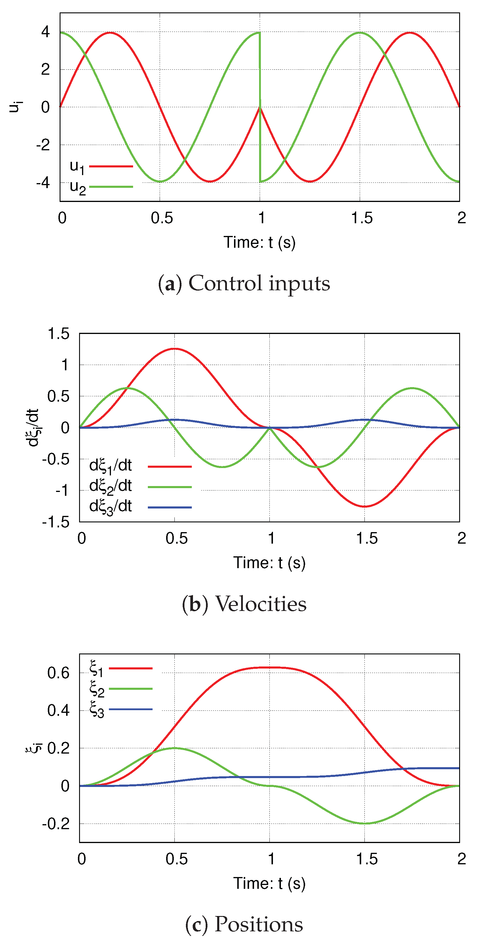
Figure 2.
Trajectories. Only (a) is derived from Reference [33].
Figure 2.
Trajectories. Only (a) is derived from Reference [33].
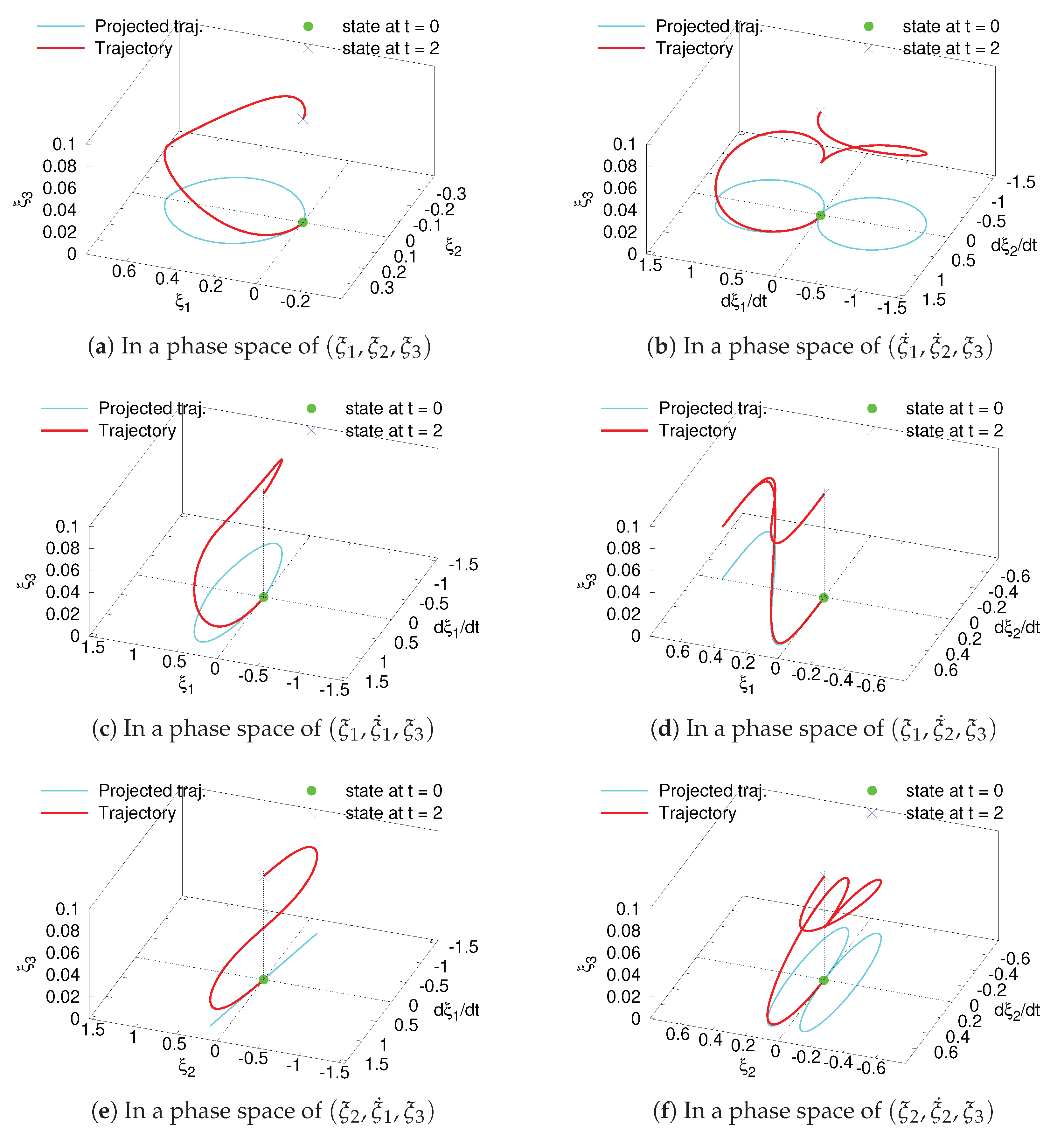
Figure 3.
Time plots.

Figure 4.
Trajectories.

Figure 5.
The algorithm of motion planning.
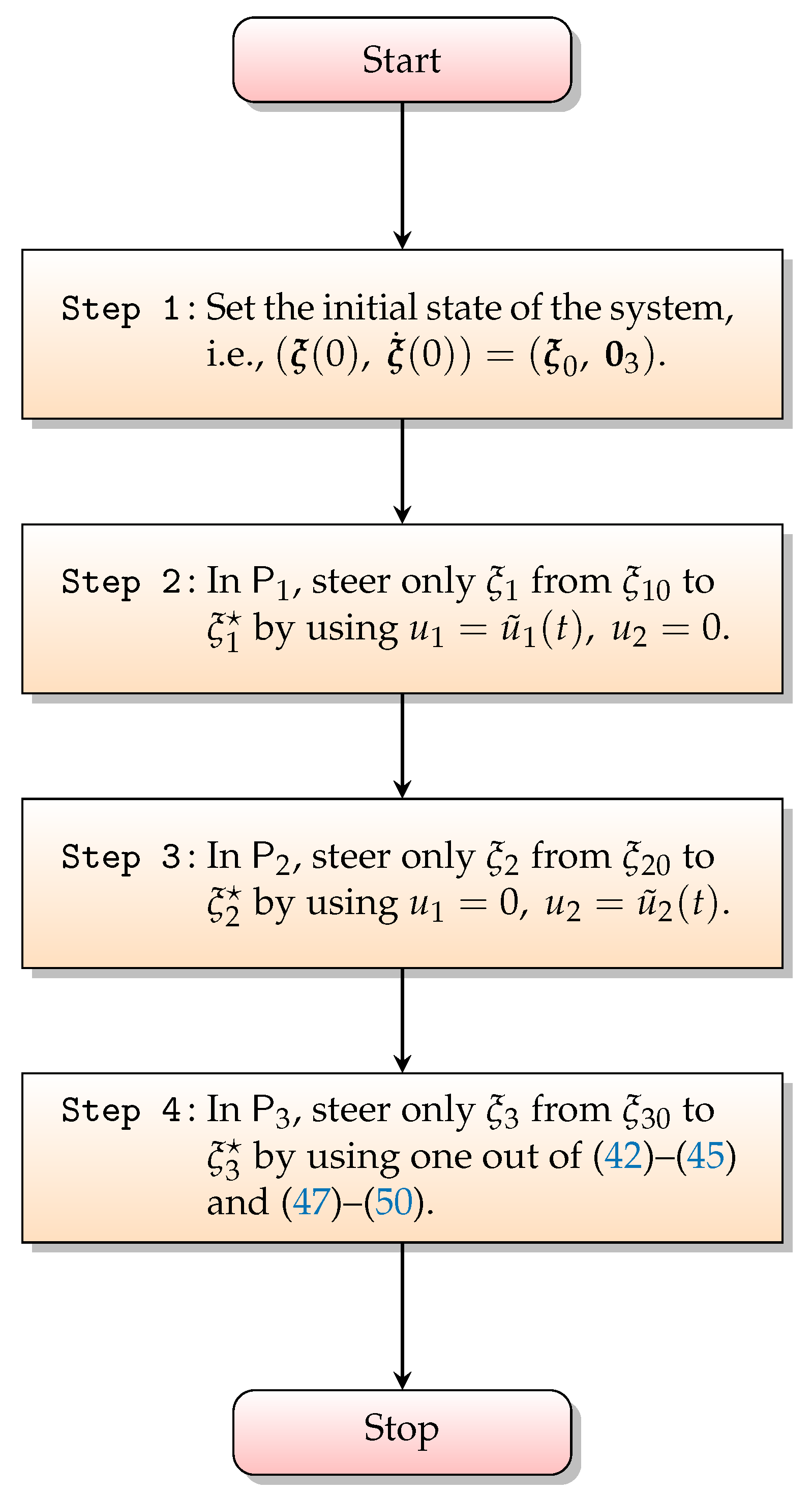
Figure 6.
Time plots.
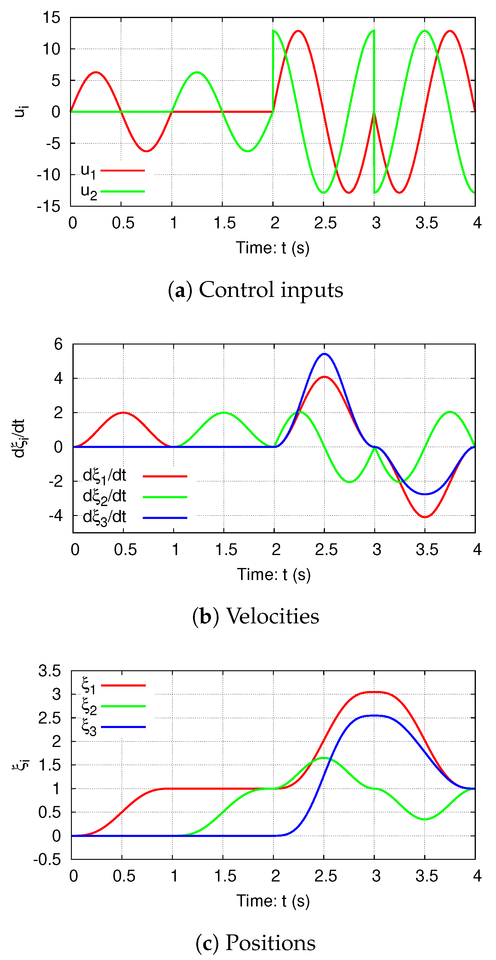
Figure 7.
A three-joint manipulator with passive third joint, derived from Reference [29].
Figure 7.
A three-joint manipulator with passive third joint, derived from Reference [29].
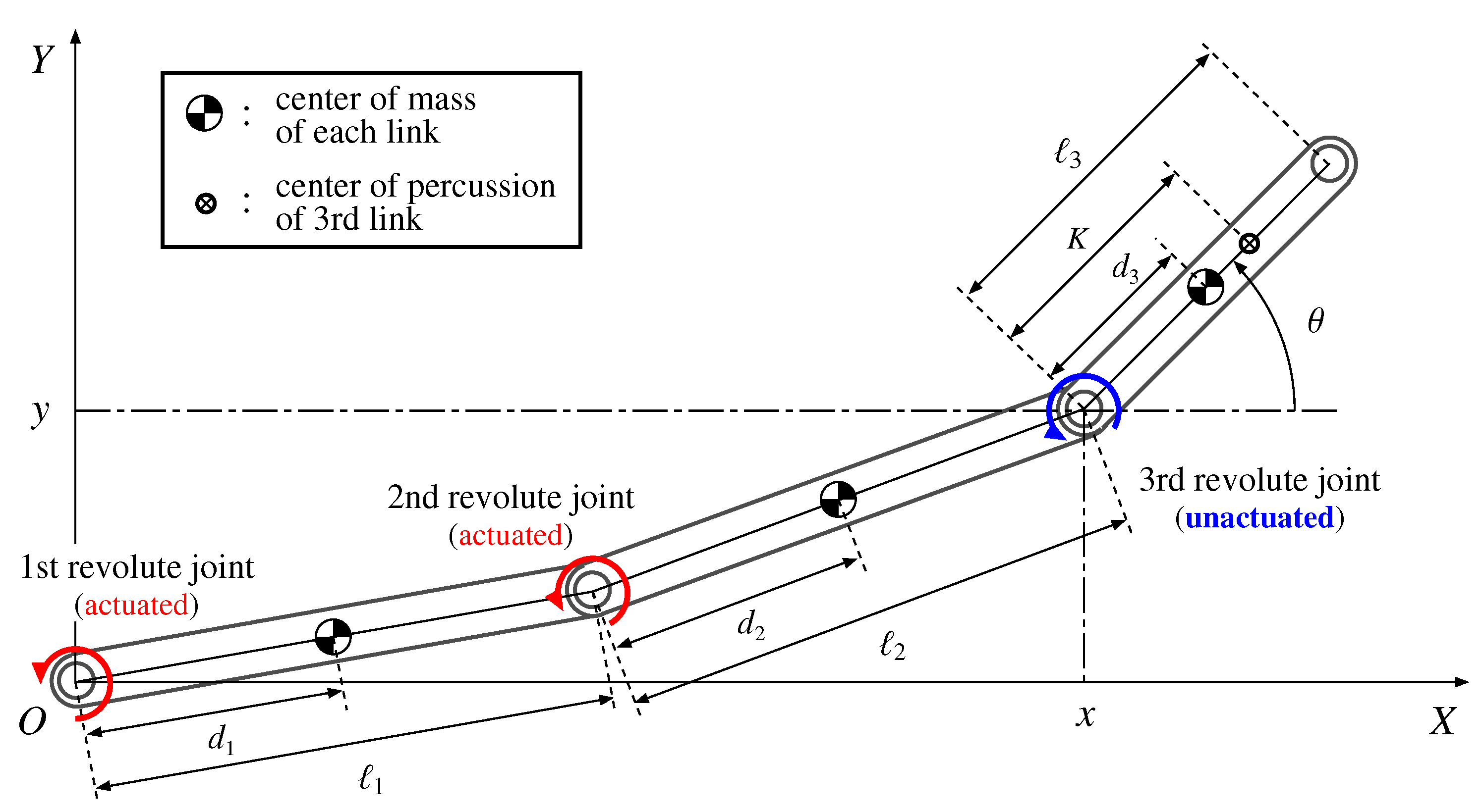
Figure 8.
Diagram for holonomy-based motion planning with (68) and (69).
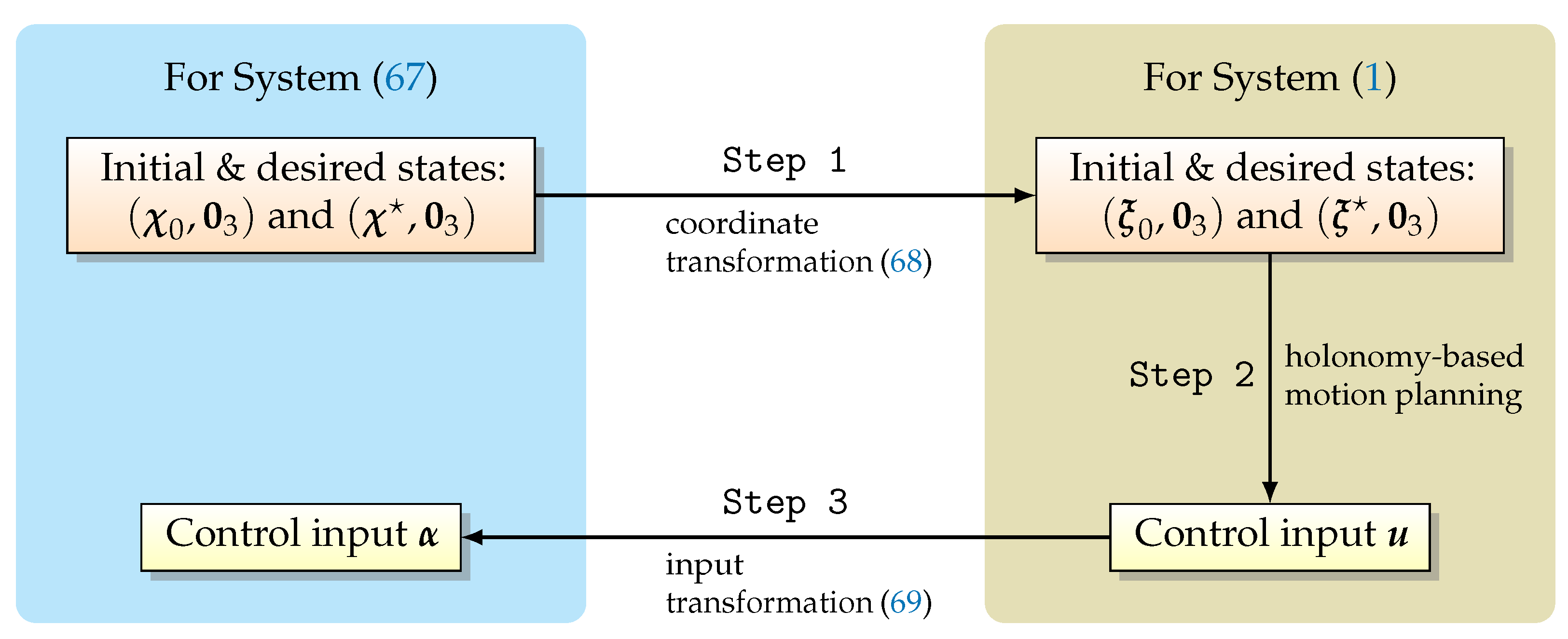
Figure 9.
Time plots.
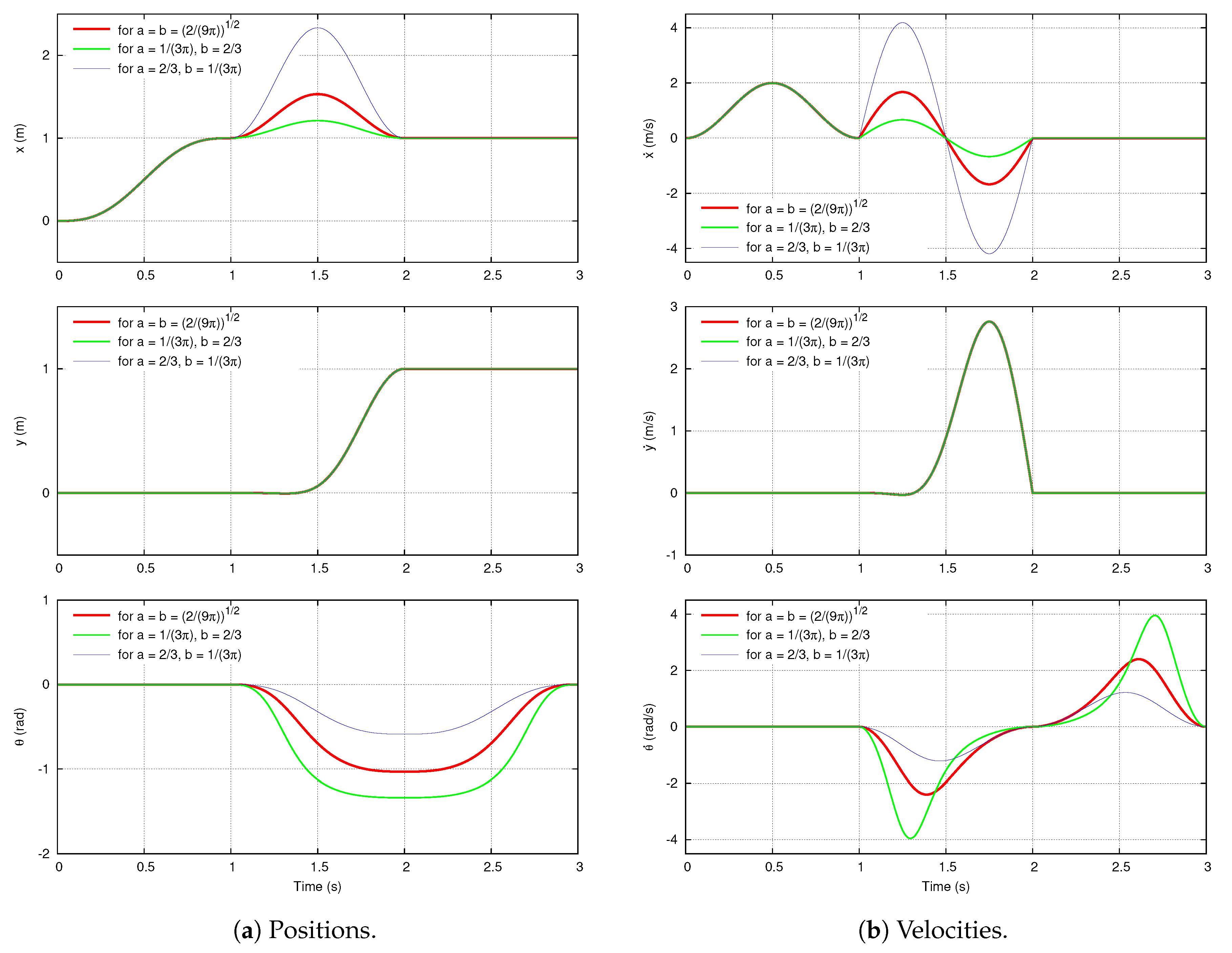
Figure 10.
Time plot of control inputs.

Figure 11.
Motion trajectories of the third link.


Table 1.
Comparison of conventional control approaches.
| Constraints | Reference | Canonical Form | Application | Control Approach | Explicit Use of Holonomy |
|---|---|---|---|---|---|
| [14] | Partially FL | Knife-edge, etc. | MP w/sinusoids | Yes | |
| [20] | 1st-order CF | Vehicle, etc. | MP w/sinusoids | Yes | |
| [1] | 1st-order CF | Multifingered robot hand | MP w/sinusoids | Yes | |
| [15] | Left-invariant | — | MP w/sinusoids | Yes | |
| [21] | Partially FL | Acrobot, etc. | Stab. by nonlinear FB | No | |
| [22] | 1st-order CF | Unicycle robot | Traj. tracking | No | |
| Kinematic | [18] | 1st-order non-CF | — | Stab. by Switched FB | Yes |
| [19] | Cross CF | — | Stab. by Switched FB | Yes | |
| [16] | — | Knife-edge | MP | Yes | |
| [17] | — | Rolling disk | MP | Yes | |
| [23] | 1st-order CF | Firetruck, etc. | Stab. by AISMC | No | |
| [24] | — | Rolling disk | Traj. tracking | No | |
| [7] | — | R-R UAM | Stab. to EM | No | |
| [11] | — | Surface vehicle | Stab. to EM | No | |
| [8] | 2nd-order CF | 2P-R UAM | Stab. to traj. | No | |
| [10] | 3rd-link’s acc. | 2R-R UAM | Stab. to composite traj. | No | |
| [9] | 2nd-order CF | 2R-R UAM | Traj. design (≈ MP) | No | |
| [25] | 2nd-order CF | 2P-R UAM | Stab. by discont. FB w/non-regular FL | No | |
| [26] | Last-link’s PFL | X-R UAM | Traj. tracking w/dynamic FL | No | |
| Dynamic | [27,28] | 2nd-order CF | 2P-R UAM | Traj. tracking w/cascaded BS | No |
| [28] | 2nd-order CF | 2R-R UAM | Stab. by Homogeneous FB | No | |
| [29] | port-Hamiltonian | 2R-R UAM | Stab. by IDA-PBC | No | |
| [30] | 2nd-order CF | 2P-R UAM | Traj. tracking & stab. | No | |
| [13] | 2nd-order CF | Underactuated AUV | Stab. by discontinuous FB | No | |
| [31] | 2nd-order CF | — | Stab. based on MPC | No | |
| [32] | 2nd-order CF | Underactuated hovercraft | Stab. by Hölder continuous FB | No | |
| [23] | 2nd-order CF | 2P-R UAM | Stab. by AISMC | No | |
| This paper | 2nd-order CF | 2R-R UAM | MP w/sinusoids | Yes | |
| 3rd | [23] | 3rd-order CF | 2P-R UAM w/jerk | Stab. by AISMC | No |
* Note: As for the type of UAM, this table adopts the same notation as in Reference [26]. For instance, X-R means that the first actuated joints are prismatic (P) or revolute (R) and the last unactuated joint is revolute (R).
Table 2.
Definition of main variables and parameters.
| : (relative) angle of the i-th joint (); | |
| : torque for the i-th joint (); | |
| : length of the i-th link (); | |
| : distance between the i-th joint and the center of mass of the i-th link (); | |
| : mass of the i-th link (); | |
| : moment of inertia mass of the i-th link (); | |
| K | : distance between the third joint and the center of percussion of the third link; |
| : position of the center of percussion of the third link in the frame ; | |
| : orientation of the third link with respect to the X-axis; | |
| : linear acceleration along the third link; | |
| : angular acceleration with respect to . |
© 2019 by the author. Licensee MDPI, Basel, Switzerland. This article is an open access article distributed under the terms and conditions of the Creative Commons Attribution (CC BY) license (http://creativecommons.org/licenses/by/4.0/).
Share and Cite
MDPI and ACS Style
Ito, M. Motion Planning of a Second-Order Nonholonomic Chained Form System Based on Holonomy Extraction. Electronics 2019, 8, 1337. https://doi.org/10.3390/electronics8111337
AMA Style
Ito M. Motion Planning of a Second-Order Nonholonomic Chained Form System Based on Holonomy Extraction. Electronics. 2019; 8(11):1337. https://doi.org/10.3390/electronics8111337
Chicago/Turabian StyleIto, Masahide. 2019. "Motion Planning of a Second-Order Nonholonomic Chained Form System Based on Holonomy Extraction" Electronics 8, no. 11: 1337. https://doi.org/10.3390/electronics8111337
Note that from the first issue of 2016, this journal uses article numbers instead of page numbers. See further details here.