SDR Based Indoor Beacon Localization Using 3D Probabilistic Multipath Exploitation and Deep Learning


1
Department of Electrical Engineering, Pennsylvania State University, University Park, PA 16802, USA
2
Applied Research Laboratory, Pennsylvania State University, University Park, PA 16802, USA
*
Author to whom correspondence should be addressed.
Electronics 2019, 8(11), 1323; https://doi.org/10.3390/electronics8111323
Submission received: 28 October 2019
/
Revised: 6 November 2019
/
Accepted: 7 November 2019
/
Published: 10 November 2019
(This article belongs to the Special Issue Indoor Localization: Technologies and Challenges)
Abstract
:Wireless indoor positioning systems (IPS) are ever-growing as traditional global positioning systems (GPS) are ineffective due to non-line-of-sight (NLoS) signal propagation. In this paper, we present a novel approach to learning three-dimensional (3D) multipath channel characteristics in a probabilistic manner for providing high performance indoor localization of wireless beacons. The proposed system employs a single triad dipole vector sensor (TDVS) for polarization diversity, a deep learning model deemed the denoising autoencoder to extract unique fingerprints from 3D multipath channel information, and a probabilistic k-nearest-neighbor (PkNN) to exploit the 3D multipath characteristics. The proposed system is the first to exploit 3D multipath channel characteristics for indoor wireless beacon localization via vector sensing methodologies, a software defined radio (SDR) platform, and multipath channel estimation.
1. Introduction
Localization is an essential procedure needed for mobile wireless communications. The deficiency of GPS due to poor signal propagation characteristics in indoor environments leads to the requirement of developing methods for indoor localization. Traditional IPS algorithms for commercial applications leverage off-the-shelf equipment and WiFi access points (APs) as their integration into pre-existing systems is feasible and can grant accurate positioning results. Critical applications, however, such as search and rescue missions or intrusion detection and tracking in secure facilities demand high localization performance, system reliability, and frequency versatility; leading to inabilities in leveraging commercially available equipment while requiring specific system designs on low-cost platforms for potential mass production. At this point, there have been immense developments in the IPS domain that leverage pre-built commercially available infrastructure such as WiFi to perform indoor positioning. There are two commonalities between all of these developments that conform either to received signal strength (RSS) or channel state information (CSI) based localization, both of which employ machine learning and fingerprinting to obtain location estimates, however none of which considers cross-polarized links (i.e., conditions where the transmitter and receiver are not the same polarization).
RSS based localization has been evaluated with conventional machine learning procedures such as k-nearest-neighbor to solve the indoor localization problem with pre-existing WiFi systems and indoor radio frequency (RF) fingerprinting (i.e., measuring RSS at finite points inside of a room) [1,2,3]. Other methodologies have looked into the employment of deep learning for obtaining and extracting rich features embedded in measured RSS signatures via deep traditional and denoising autoencoding [4,5]. The procedures developed by DABILin [5] leverage Bluetooth low-energy devices and deep neural networks to learn spatial correlations between training and testing points by training a denoising autoencoder at each individual location and measuring Euclidean distance relative to testing points. DABIL produced localization errors around 1 m with 10 Bluetooth receivers placed in LoS conditions as the transmitter, and receiver polarization is undocumented.
For CSI based localization systems, much emphasis has been placed on the improved localization performance over RSS based approaches as more fine-grained information embedded within CSI tends towards spatial learning via multipath scattering. The predominant system employed for monitoring or sniffing wireless local access networks (WLANs), i.e., WiFi, is the Intel 5300 network interface card (NIC), which computes the CSI from received WLAN packets. The CSI is commonly extracted and analyzed by machine learning algorithms when performing offline (i.e., training) and online (i.e., testing) stages of indoor localization. One approach explored probabilistic location estimation on measured CSI magnitude packets to construct a propagation model [6]. Other approaches utilize the CSI magnitude extracted by the WiFi 5300 NICs and deep learning to perform effective indoor localization deemed DeepPOS, DNNFi, and DeepFi, respectively [7,8,9]. Building upon the CSI magnitude effectiveness and deep learning, PhaseFi was explored to extract phase information from the Intel 5300 NIC, realizing a minimal modification to the DeepFi learning protocol via change in the input feature vectors while leveraging a linear array of three antennas [10]. Nonetheless, both DeepFi and PhaseFi realized localization errors around 1 m in performance with a restricted Boltzmann machine (RBM), however once again with APs positioned in LoS conditions with non-existent documentation on the polarization state of the transmitters and receivers.
To date, minimal research has been conducted in SDR platforms for indoor localization. In [11], RSS was captured for both GSM and WiFi using USRP E310, and a WiFi Pineapple as a least squares (LS) algorithm was employed for distance estimation realizing localization errors on the order of 5 m. Similarly, a USRP device and LS distance estimation approach was employed in [12] for monitoring the uplink RSS of GSM waveforms using openBTS software for realization of GSM base stations. Another physical estimation of location was employed in [13] via time difference of arrival (TDoA) and four spatially distributed receivers. The results documented localization performance of sub-0.5 m in an undocumented environment. Finally, the most recent research expressed in [14] demonstrated one of the first machine learning based WiFi localizing SDR platforms. The SDR leveraged simultaneous RSS and CSI in a LabVIEW aided system cascaded with a convolutional neural network to achieve approximately 1 m of localization error. The main operation of the system was to mimic a WLAN Intel 5300 NIC, in which extracted features were validated by NIC 5300 measurements at a rate of 500 packets per minute. Nevertheless, the system documents one of the first SDR based WiFi indoor localization methods that employ deep learning for location estimation under predominantly LoS conditions.
This work proposes an SDR based localization procedure that can rapidly extract 3D multipath CSI and perform indoor localization via PkNN and deep learning at rates relative to the link’s time-bandwidth product. In the case of this work, a bandwidth of 5 MHz is used with a BPSK beacon frame of 2 ms realizing 10,000 times improvement in packet realization rates when compared to the approach in [14]. The selected bandwidth and digital modulation are not required as the designed approach implements a matched filter methodology that is agnostic to frequency, bandwidth, and transmitted waveform so long as the SDR can tolerate such characteristics. The work builds upon [15,16], however now in relation to indoor localization of an arbitrary binary phase shift keying (BPSK) beacon waveform and vector sensor receiver. The purpose of the document is to benchmark the state of SDR based localization platforms to convey the importance of obtaining 3D multipath characteristics in order to achieve high localization accuracy in NLoS environmental conditions with only one receiver position. Since most of the aforementioned localization algorithms are defined in LoS conditions, the proposed system is compared to Horus (i.e., RSS based methods), DABIL (i.e., deep learning based RSS method), and DeepFi (i.e., deep learning based CSI method) under an LoS constraint (i.e., considered to have multiple receiver positions for synchronized beacon reception); whereas, the proposed method is left unconstrained (i.e., only leverages one receiver position). The first statement of purpose evaluates the localization performance of the proposed method of 3D multipath exploitation without deep learning under idealized conditions where interference is not present via simulation. Degradation in the proposed approach is expressed, in which a deep learning approach is developed to combat the presence of interference that can arise in SDR conditions. After discussing and comparing all methodologies via idealized simulation, an Ettus X310 SDR platform is cascaded with a designed vector sensing antenna in the indoor environment for experimental verification of the proposed localization algorithm.
2. 3D Multipath Estimation and Probabilistic Learning
The process of performing indoor localization is two-fold starting with multipath channel estimation based on the knowledge of the transmitted BPSK beacon frame and ending with probabilistic machine learning. The 3D multipath information is unique as the information encompasses spatial correlations related to the physical emitter’s location in the indoor environment. Expanding on this, the development of a triad dipole vector sensor (TDVS) antenna for the purposes of this work is different than that used in common practice, in which the vector sensor is used for simplistic direction of arrival (DoA) estimation [17,18,19]. The designed TDVS for all intents and purposes was designed within this work to extract polarization based features embedded within electromagnetic diffuse scattering received at the TDVS in complex indoor environments.
2.1. 3D CSI Estimation
The extraction of 3D multipath starts at the antenna stage, in which three orthogonally co-located half-wave dipole antennas are used to acquire all x-, y-, and z-dimensional characteristics of the space-time multipath channel defined in [15,20]. More specifically, the transmitted BPSK sequence at 3D location l in Cartesian coordinates (,,) impinges the TDVS in the form:
with denoting an orthogonal element of the vector sensor, K describing the cardinality of the space-time channel, the number of elements of the TDVS (i.e., three), the complex baseband modulated BPSK sequence, w denoting complex additive white Gaussian noise, H describing the complex space-time wireless channel correlated with , and used for maintaining symmetrical energy between baseband and bandpass signal representations. Using the received 3D space-time wireless signal, channel estimation is performed in order to estimate the wireless channel. Since the beacon BPSK sequence, , is a known sequence at the receiver, the receiver can leverage such knowledge to estimate the channel impulse response (CIR) of the 3D wireless channel at the receiver. The method employed here builds upon the representation of the received 3D signal described in (1), where the channel estimation procedure results in:
with denoting statistical expectation, denoting the Hermitian complex conjugate transpose, the statistical mean of the BPSK beacon frame , and describing the covariance matrix of the BPSK beacon frame. Depending on the approximated number of multipath taps (K), the estimate of the wireless channel estimate in (2) appears as:
where C is the estimated covariance matrix and is the measured cross-correlation vector. Leveraging the CSI information achieved by (4), the resulting feature vectors are created and stored for machine learning based on the magnitude of the estimated CSI coefficients. A feature vector is then constructed based on the magnitude coefficients of the 3D channel in the form:
where denotes magnitude and denotes complex conjugate transpose.
2.2. Probabilistic Localization Algorithm
Similar to [5], the designed localization algorithm employed on the extracted 3D CSI is based on Bayes’ law and employs a probabilistic k-nearest-neighbor (PkNN) algorithm. The algorithm is designed to measure the a posteriori probability of a given reference location l relative to an input 3D CSI feature vector , expressed as:
where is the prior probability. A relaxation is made to (5) by assuming a uniform prior probability such that equally likely probabilities are distributed across all reference locations within the training set. The resulting form of (5) then becomes:
Leveraging (6), a resulting probabilistic kNN is defined relative to the conditional probability and an distance measurement. The definition of the conditional probability in this work is based on an exponential function relative to an distance measurement between two feature vector points of the form:
where is a scaling parameter on the variance, , of the distance (i.e., similarity between and ), with and left undefined for now, however representative of training and testing set information. The definition of the scaling parameter, , in (7) within this work is empirically defined based on realizable characteristics of the similarity measure between and and spatial separation, all of which is defined in forthcoming sections. The resulting localization algorithm then employs a probabilistic estimate of the location of the emitter via the weighted average of K reference locations:
where denotes the estimated position of the emitter in 2D coordinates, denotes the kth 2D reference coordinate, and K denotes the number of neighbors employed in the positioning algorithm. The proposed probabilistic algorithm in (8) ensures a positioning system that can give a level of certainty to the location estimate. Such a system has advantages over traditional machine learning procedures as the conditional probability allows for probabilistic thresholding to be enforced relative to a probabilistic confidence.
3. Deep Learning and Denoising Autoencoder
As continuous BPSK beacon frames are recorded for indoor localization in both the training and testing stages, there are various sources of error that can arise in the measurement process. Two of the most common types of error in the packet monitoring process for SDR platforms are packet loss (i.e., dropped packets) and spurious interference caused by other emitters in the environment. If the training stage assumes negligence of potential packet loss or interference presence in the testing stage of the localization procedure, then degradation in localization results typically follows suit. It has been proven that deep learning can combat such random processes via unsupervised projections that lead towards a learned representation of the statistical distribution encompassing the input feature vectors to the deep learning process [5,7,8,9,10].
In this work, a deep denoising autoencoder is employed in order to minimize the impact of random fluctuations in the packet reception process. By design, the autoencoder projects a given feature vector input to a bottleneck in an encoding procedure. After projecting to the bottleneck, the autoencoder network employs a decoding layer that mirrors the encoding layer. This mirroring procedure leads to a reconstruction of the input based on the weights of the neural network. A loss function is then employed at the output that compares the input features to that of the reconstructed features at the output of the autoencoder. This procedure is iteratively performed via backpropagation until an error criterion is met. The minimization of this error function is equivalent to maximizing the minimum mutual information between the input and the reconstruction [21].
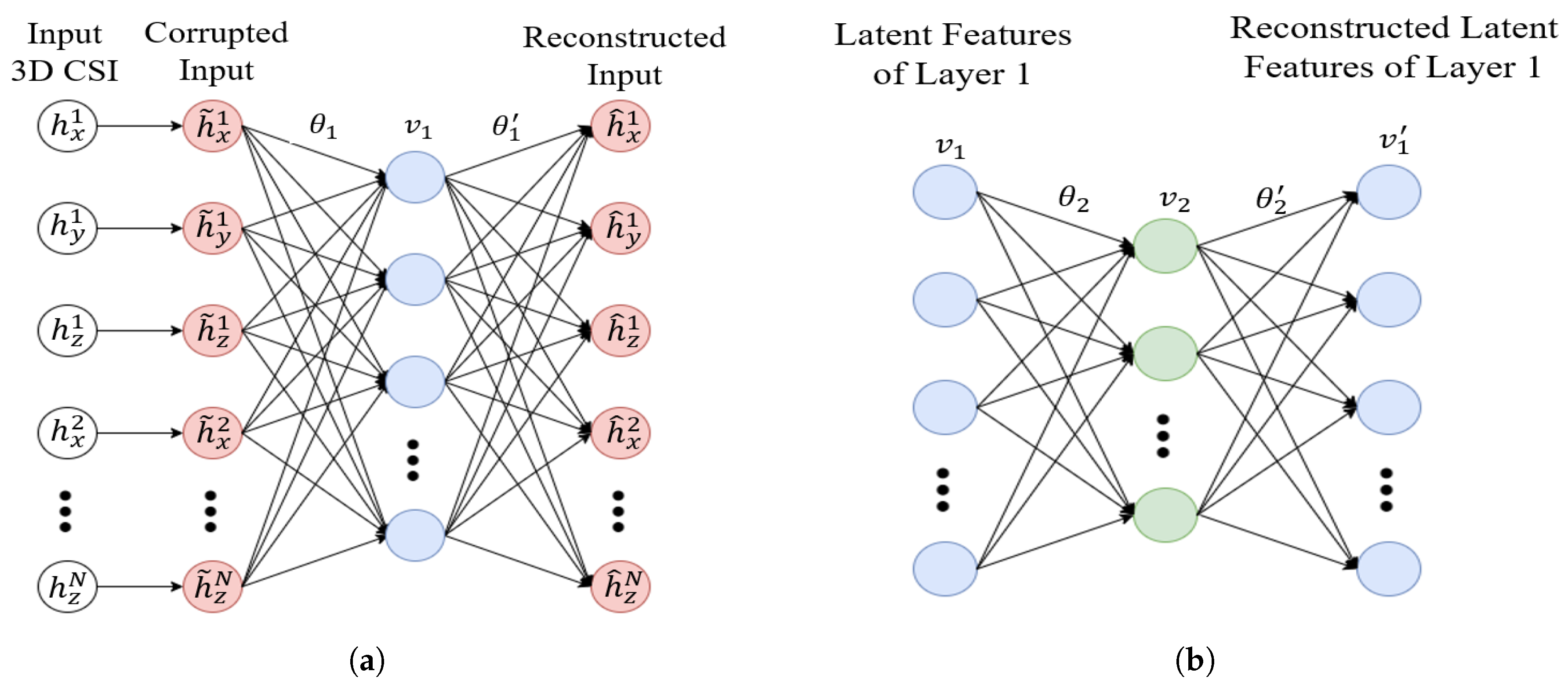
It has been shown that features learned by a traditional autoencoder converge to principal components [22]. The only difficulty with using principal components is that the features learned are linear representations of the input, in which, for the case of packet loss and interference for the SDR platform, such random fluctuations are non-linear. Thus, the proposed method for minimizing the impact of non-linear fluctuations is a deep denoising autoencoder (DAE) that learns the latent (i.e., stochastic) features of the input vector. The biggest difference between the traditional and denoising autoencoder is the loss function. For the case of the denoising autoencoder, the input features are synthetically corrupted in the training stage. The corrupted features are then the input to the denoising autoencoder, in which the neurons of the autoencoder are adaptively updated relative to a reconstructed output that is compared to the ground truth feature vector. This comparison forces the neurons to take on stochastic values that conform to the distribution of the input features [21]. An example architecture of a two-layer denoising autoencoder with a 3D CSI feature vector as input is depicted by Figure 1.
Construction of the denoising autoencoder structure is performed by stacking multiple autoencoders sequentially, depicted graphically in Figure 2. The learning process starts with the first hidden layer, where the starting stage is a deterministic mapping (i.e., encoding) of the corrupted CSI features to a hidden representation as:
where is a weighting matrix of the first transformation (i.e., hidden layer), is the corrupted CSI input feature vector, is an activation function, and is the bias vector of the first hidden layer of the network [21]. Corruption is traditionally performed via forcing input features to zero or through the addition of additive white Gaussian noise. The corruption process used in this work is defined in Section 4.3.1. The activation function, , is defined as a logistic sigmoid function expressed relative to the inputs defined in (9) as:
A decoding of the transformation performed in (10) is then enforced to for reconstruction of the input as:
where is the weighting matrix of the mirror hidden layer and is the reconstructed input feature vector based on the corrupted input. It is apparent that the denoising autoencoder takes the corrupted input and looks to map the input to an uncorrupted version through the transformation procedure. A cost function (i.e., loss function) is then constructed based on the reconstructed version and the training sample vectors as found (9) and (11) for converging the first hidden layer weights of the denoising autoencoder as:
The autoencoder can be made more sophisticated by specifying subsequent mappings (i.e., transformations) through the addition of more hidden layers via stacking autoencoders. When adding a second layer, the encoder of the second hidden layer appears in the form:
where the decoding at the mirror layer of the second encoder in (13) is constructed as:
The corresponding loss function of the mirror layer decoded by the second hidden layer in (14) is then employed to converge the weights of the second layer of the denoising autoencoder, such that the second layer loss function is defined as:
This sequential mapping of each layer would then be carried out for every added hidden layer in the stacked denoising autoencoder network as each subsequent reconstruction has an accompanied reconstruction loss function similar to those defined in (12) and (15). Observation of the loss function defined in (12) suggests a simplistic alternative input to the conditional probability defined in (7). This is the intuition of the reconstruction procedure and loss function of the denoising autoencoder described in this work.
4. Indoor Localization Model
The comparative process of DeepFi, DABIL, Horus (i.e., RSS based), and the proposed 3D CSI method expressed in this work was conducted in an electromagnetic solver for an idealized analysis. The software package used was Wireless InSite, a sophisticated electromagnetic ray-tracing tool used for modeling indoor wireless signal propagation. The ray-tracing tool was used to evaluate the performance of commonly referenced localization algorithms in the IPS literature. The simulation model served as the mechanism for comparing all algorithms to the proposed method and looked to demonstrate the importance of polarization effects on IPS algorithms. The main objective of the simulation model, however, was to ensure the parameters demonstrated in the simulated environment had a similar correspondence to the parameters used in the true indoor environment.
4.1. Indoor Model
The synthetic indoor environment created in Wireless InSite was to match the replica of the experimental indoor environment with the designed SDR platform. The building dimensions used in replicating the experimental environment were 23 m in length, 9 m in width, and 3 m in height. The total number of rooms inside the environment was eight. The materialistic specifications of the simulated indoor environment also followed the experimental environment as the walls were created to have the dielectric properties of brick, the floor modeled as concrete, closed doors modeled with metallic properties, and windows constructed with the dielectric properties of glass. A grid of transmitters was then scattered throughout the designed indoor model at a spacing of 0.5 m. A total of 2013 emitters were placed inside of the environment at a fixed height of 1.25 m, which remained static throughout the entirety of the simulation. The transmitters were then separated into groups of training and testing sets. For the training set, a total of 1461 transmitters were used in the offline training procedure, leaving 552 for the testing stage, approximating a 70/30 training and testing split.
In order to realize all algorithms, the set number of receivers used in the simulation can vary. Thus, in order to stay consistent with the procedures defined in DeepFi, DABIL, and Horus, the number of receivers and conditions of the environment needed to remain relatively consistency. Since the aforementioned algorithms were employed in LoS conditions, the set number of receivers used inside of the environment was equivalent to the total number of rooms (i.e., eight), all of which were mounted to the ceiling at a height of 3 m. This requirement ensured that there was always a receiver gathering LoS signal characteristics at all times regardless of the emitter’s position. In contrast to this notion of always receiving an LoS component, the proposed method did not require LoS signal propagation, and so, the comparisons between the approaches performed in literature were leveraging eight receivers, whereas the proposed approach employed only a single vector sensor antenna. Nonetheless, the simulated environment is depicted by Figure 3. The one caveat in the simulation, however, was the selection of optimal location to place the TDVS antenna. Based on the selected room for which the receiver was placed, the localization performance can vary for CSI or RSS based methods due to the geometrical properties of the scattering phenomena along the propagation path [23]. Thus, we looked at the TDVS at all eight locations to demonstrate the fluctuations that could occur as a function of the placement of the TDVS receiver.
In regards to the requested output features for each algorithm, the different types of features were extracted comparable to those employed in DeepFi, DABIL, and Horus. For DeepFi, 25 CSI features were extracted for the single antenna case of the Intel 5300 NIC, whereas 75 were extracted for the proposed approach (i.e., 25 per element of the TDVS). The number of CSI elements to be estimated was computed by the software package such that full representation of the scattering was achieved at all points in relation to the complex impulse response. For DABIL and Horus, raw RSS was extracted. As far as the transmitter and receiver properties, a carrier frequency of 915 MHz was used such that realization of the model could be achieved in the unlicensed ISM band and for optimal resonance with the designed TDVS. We note that the selected 915 MHz signal was not imperative as any selected carrier would work with the designed localization approach. In the case of the receivers used to model the methods in the literature, a half-wave dipole of vertical polarization was employed; whereas for the proposed approach, a vector sensing omnidirectional antenna was employed. Furthermore, in order to demonstrate the importance of polarization impacts on the IPS algorithms, the transmitter was modeled as a co-polarized emitter with the receiver sets, as well as in the cross-polarized state (i.e., horizontally polarized emission). Regarding the transmit waveform, a BPSK beacon frame was used similar to that used in the experimentation.
4.2. Simulation Results
After modeling the simulation for both transmitter polarization states, all pertinent features were extracted and fed to their respective localization algorithms. For the proposed approach of localization, the probabilistic kNN required the selection of the scaling parameter . With only knowledge of the training samples, an empirical estimate of the optimal scaling parameter was determined by measuring ground truth distance between all 3D CSI feature vectors and relating the distance to the physical separation of training emitters. A depiction of the process for selecting the optimal scaling parameter is given by Figure 4 for a receiver located in Office . The results demonstrated the deviation that occurred as the distance increased with RSS features relative to increased spatial separation between all existing emitter points in the training set. This empirically measured phenomena was similar to what was realized by [5] for RSS, where the distances increased as a function of physical separations between training locations. Nonetheless, observation of the physical distance versus distance revealed information about the optimum selection of . An empirical solution to the value was found by mapping the same distances to the conditional probability . It is apparent by the mapping that the selection of for would give high probability to emitters with less than for both horizontal and vertical polarization states of the transmitter, equivalent to the selection of emitters within 1 m of proximity.
Leveraging the optimum scaling parameter, localization can be performed on the testing points in a probabilistic manner. The results were first demonstrated without using the deep learning approach to localizing the emitters with the 3D CSI, in which only PkNN was in effect. The rationale behind not using the denoising autoencoder with the 3D CSI method was to demonstrate that deep learning was not required in order to obtain a high level of precision in localization with the proposed 3D CSI approach as ideal conditions were assumed such that interference or loss of packets was negligible. The results of the localization procedure of the 3D CSI approach with the TDVS for each individual room of the simulated environment are demonstrated by Figure 5 for both vertically and horizontally polarized transmitters as the localization error metric is defined as:
where represents the physical distance error, is the PkNN estimate of the emitter in the x-dimension, x denotes the ground truth, is the estimate of the y-dimensional coordinate, and again y is the ground truth. The results demonstrate that the optimum placement of the TDVS antenna with the 3D CSI feature approach varied based on the transmitter polarization. For the vertically polarized condition, the best TDVS position was in Office , with a representative average localization error based on (16) of 0.53 m. A complete table of the statistics is demonstrated by Table 1.
Considering the statistics and results demonstrated by Table 1 and Figure 5, it is evident that polarization had a direct impact on the 3D CSI approach regarding the optimum placement of the TDVS receiver. This was due to the change in the diffuse scattering that occurred when polarization transitions happened at the transmitter. For simplicity, only the results of the TDVS in Office are considered from this point moving forward in order to compare the performance with the other proposed algorithms in the literature. The results for the comparison are depicted by Figure 6. The results demonstrated the robustness of the proposed 3D CSI approach in which the single TDVS receiver was capable of outperforming all other approaches that leveraged all eight receivers simultaneously. Another interesting trend between all approaches was the degradation of all approaches that did not employ polarization diversity. As the transmitter operated in the cross-polarized domain, methods such as DeepFi, DABIL, and Horus degraded severely in the localization performance, whereas the proposed method was fairly stabilized due to the polarization diversity it offered the receiver, which resulted in a maintained magnitude response for the channel estimate. The final statistics comparing the approaches can be found in Table 2.
4.3. Interference Impacts on 3D CSI and Denoising Autoencoder
The aforementioned results demonstrated the effectiveness of the proposed localization method in comparison with other localization approaches found in the literature. The underlying assumptions of the aforementioned localization results were that the training and testing sets had purely representative features of the CSI or RSS from the locations being tested. An issue with this underlying assumption is that this is almost never the case when attempting to integrate simulation models into experimental infrastructure, as spurious interference is highly likely in unlicensed radio frequency bands. Therefore, an exploration of the impact that interference has on the proposed 3D CSI localization approach was evaluated. Since the TDVS 3D CSI system was intended to be integrated onto an SDR platform, it was evident that there would be dwelling periods in which an interfering source could potentially impinge the TDVS receiver in the same time-frame as packets coming from the true source location. Thus, it is possible that some collects could have higher amounts of interference than other locations, leading to the potential scenario where one might train a machine learning or deep learning model on an interference-free dataset, however attempting to test on received packets that are corrupted with interference containing a certain amount of corruption.
4.3.1. Interference Generation
The creation of the interference needed to maintain some form of realistic representation of a scenario found in practice; thus, it was developed based on the path loss model constructed in [24]. Starting with the path loss endured on the interfering signal when propagating to the TDVS antenna, the received interference power at the TDVS receiver was of the form:
where is the received interference power in dB, is the radiated power of the interfering source in dB, and is the propagation loss in dB. The expression of the path loss is represented as:
where d is the physical distance of the TDVS receiver to the interfering source in meters and is the wavelength of the interfering source. After satisfying the path loss model expressed by (17) and (18), the final constraint required to model the interference in a realistic manner was to consider the interference time relative to the true BPSK beacon frame (i.e., up-time of the interfering source). Since modeling the sporadic fluctuations of the random process realized by radio frequency interference was difficult, the simulated model made constraints on the state space of possible interference parameterizations. For the case of training, the simulation model assumed interference was non-existent. This was a practical assumption as interference can be minimized or monitored in the training stage. When exploring the testing stage, it was assumed that the localization model was generated and placed in a state to localize emitters in an online phase. In this case, interference cannot be avoided as easily, and so, we looked to explore the impact that the presence of interference might have on the developed localization model.
Since path loss was accounted for, the final stage was to model how the interference impacted the beacon frame from a time interval standpoint. For the simulation model, the received testing frames to be localized inside of the indoor environment are modeled as:
as is defined as a complex tonal time series expressed as:
where denotes the interference duration (i.e., corruption time ), M denotes the length of the interference signal in samples, denotes the time duration of the BPSK beacon frame in (19), is the center frequency of the interfering signal, is the interference scaling variance relative to the path loss model realization of interference power received, and is a random phase variable . The interference was varied from low corruption time (i.e., ) to complete corruption for the transmitted BPSK beacon frame (i.e., ).
4.3.2. Training 3D CSI Interference Based Denoising Autoencoder
The results of the 3D CSI based localization algorithm were compared to that of a developed two layer 3D CSI denoising autoencoder (DAE) when interference was present in the testing phase of localization analysis. The corruption process in the training procedure of the DAE was to inject interference into the training features similar to that defined in (19) and (20). Since the input to the path loss model required distance and power levels, the constraint was placed to only consider emitters within the maximum range of the environment from a receiver’s perspective (i.e., 20 m away), while also constraining the power levels within the maximum observable signal level of the emitter of interest (i.e., beacon source at 13 dBm).
The deep learning model was found optimum as a two layer neural network, in which 50 and 25 neurons were used in the outer and inner layers, respectively. Since it was impossible to consider all realizations of potential interference power levels that could occur in the environment, the corruption process had set the interference power to be 1 dBm for demonstration purposes of improvements that could be achieved relative to the original 3D CSI proposed. Nonetheless, the selection of the power level to train the DAE was important to be measured a priori in the real environment as it was demonstrated in upcoming results how this power selection of 1 dBm degraded if not chose adequately relative to the testing power levels. Lastly, corruption time used in training the DAE was set to 50% (i.e., M = N/2), and the distances used in training were meters away from the TDVS receiver in Office #2. The DAE was trained using a scaled conjugate gradient backpropagation method to adjust the weights of the deep learning model. A deep learning 3D CSI model was trained for every location within the training set. Each set of weights for all DAE models was stored off to be used in the testing phase where the conditional probability for the PkNN model now becomes:
where denotes the test set 3D CSI feature vector with interference corrupted features and denotes the reconstructed input (i.e., output of the DAE) based on the weights extracted in the training phase.
4.3.3. Localization Performance with Interference
The developed corruption procedure was incorporated into the test sets to evaluate any degradation from the original performance. The carrier frequency of the interfering source was placed at the center of the transmitter carrier frequency (i.e., 915 MHz). The interference power was initially set at 1 dBm to evaluate how subtle low power emissions from sporadic interference can impact the 3D CSI based localization algorithm relative to the trained 3D CSI DAE. A depiction of the localization performance for both vertically and horizontally polarized transmitters with varied corruption times is found in Figure 7. The results showed that the presence of interference in only the testing set for traditional 3D CSI method severely degraded the localization performance. Moreover, it is also noticeable that both methods degraded as the corruption percentage increases (i.e., as interference persisted throughout the entire beacon frame). Nonetheless, DAE was successfully able to minimize the impact of interference in the testing stage of localization relative to the TDVS approach, which did not consider interference.
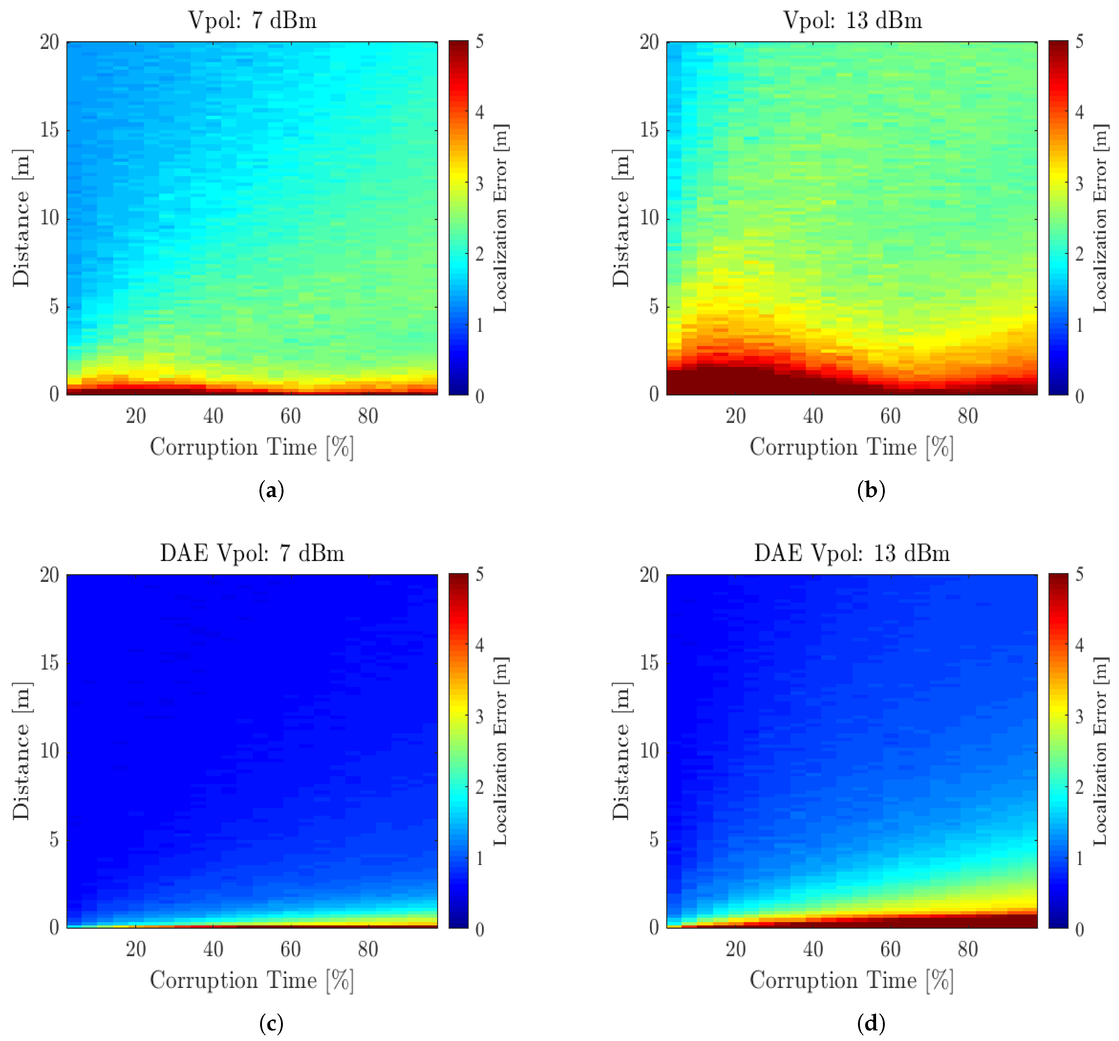
The second analysis evaluated how interference impacted localization performance as a function of distance and power in the testing stage of the trained algorithms. For the case of the selected 1 dBm training power in the DAE, it was explored how this selection was impacted by a larger interference power in the environment. The surface plots of the localization error of the two different 3D CSI approaches are demonstrated by Figure 8 and Figure 9 for both vertically and horizontally polarized transmitters with interference power at radiated levels of 7 and 13 dBm (i.e., matching the radiated power of the target beacon source). The results showed that the increased power of the interference resulted in an effective increase in the localization error for all cases, however having less impact on the DAE for both vertically and horizontally polarized transmitters. It is also apparent that the closer the emitter was to the receiver, this resulted in higher localization error. The results ensured the importance of polarization considerations as the interference can potentially yield higher error on the localization surface for horizontally polarized emitters.
The results demonstrated how the DAE could effectively stabilize the localization performance in the presence of interference from an error surface perspective and how distance, corruption time, and radiated power impacted the localization error. This implies that the presence of spurious interference at the TDVS receiver could be minimized when transitioning the 3D CSI deep learning localization algorithm into an SDR platform for real-time sensing. The results captured by Figure 10 demonstrate the average localization error as a function of stepped interference power in 1 dBm increments from 1 to 13 dBm across all possible distances and corruption times (i.e., average error of the error surfaces depicted by Figure 8 and Figure 9). The results demonstrated the improvements that can be obtained by employing the DAE versus the non-deep learning approach of 3D CSI. It was apparent that a localization improvement of 1 m in error could be obtained using the proposed DAE algorithm for both vertically and horizontally polarized transmitters in the indoor environment. This implies that the DAE was learning the latent features of the input 3D CSI in a manner that essentially filtered out the interference in the reconstruction layer. As far as we are aware, such a training for a denoising autoencoder has not been introduced until now in the literature.
5. Software Defined Radio Experimentation
The simulation models in the previous sections introduced the deep learning procedure for probabilistic emitter localization based on 3D channel state information acquired from a TDVS receiver. The simulation expressed an idealistic comparison of localization algorithms found in the literature against the proposed 3D CSI method. This section, however, only looks to address the design and implementation of the proposed localization approach on an SDR based platform. The first stage introduces the performance of the channel estimation procedure used in acquiring 3D CSI in the indoor environment on an SDR. After ensuring the effectiveness of the CSI estimation procedure, the final subsection discusses the results of the experimentation for the designed SDR based indoor localization system.
5.1. CSI Estimation
The first step in designing the localization system was to ensure that channel estimation can be obtained with the SDR platform. An Ettus X310 SDR was acquired and used for all experimentation on a Linux operating system. An arbitrary waveform generator (AWG) was acquired in order to transmit the reference BPSK beacon sequence. The demonstration of ensuring a proper estimate of the CSI for indoor localization was performed via inverse modeling (i.e., channel equalization). The proof of concept that efficient channel information can be estimated was performed via the inverse solution of removing the channel effects. Such a demonstration yielded insight that the physical bits transmitted by the wireless BPSK beacon could be estimated by the receiver in harsh indoor conditions, thus leading towards the feasibility of gathering the channel inverse information. The experiment also looked to explore the minimum number of samples required per packet in order to maximize both the number of packets transmitted per second, while also ensuring effective channel estimation.
The experiment leveraged the PropSim C8 wideband multi-channel emulator to control channel conditions and allow for channel equalization to be performed on the BPSK beacon frame. Two NLoS channel models were evaluated in the experimentation with the X310 SDR where BPSK packets of length were generated sequentially at a 5 MHz baud rate. It was assumed the beginning N samples were known prior to receiving the packets, where only the remaining bits were counted in the bit-error-rate analysis after equalization. The first NLoS channel model used in the analysis was the LTE-ETU model, in which nine Rayleigh fading channel taps were used in consideration of an outdoor Rayleigh fading channel. The second channel emulated was the WLAN ETSI Model E, which has 19 Rayleigh distributed taps for modeling indoor environments. The carrier frequency used in the experimentation was 915 MHz, the same used in the simulated model and upcoming indoor localization experimental environment. The results for the experimentation are depicted by Figure 11. The results demonstrated that a symbol length of 10,000 samples granted feasible performance at removing channel distortions induced by the C8 channel emulator for both channel models and thus was the length defined for the indoor experimentation.
Using the 10,000 sample sequence and continuing to evaluate Rayleigh fading channel effects on the transmitted BPSK sequence, a second analysis was evaluated that considered non-stationary emitter characteristics. In most literature, the fingerprinting stage for indoor localization was performed in environments where training and testing emitters were kept or assumed stationary. Any non-stationary emitters would induce Doppler shifts in received signals which could lead to increased variation in CSI characteristics. A BPSK waveform propagated through a Doppler Rayleigh fading channel had the probability of error:
where is the energy per bit, is noise power, is the Bessel function of the first kind and order zero, is the Doppler frequency induced by emitter motion, and is the symbol duration. Using this expression, various Doppler shifts were emulated with the PropSim C8 on the transmitted BPSK reference frames. The results when propagating the BPSK reference through the WLAN ETSI Model E are found in Figure 12 comparing theoretical expectations to the measured performance via C8 emulation. The results demonstrated that increased Doppler variations simply led to lesser performance in equalizing the channel, or in the case of the indoor localization, the ability to accurately estimate the CSI. Leveraging this information, all emitters were maintained in stationary positions when conducting indoor localization experimentation with the SDR as Doppler fluctuations induced by emitter motion degraded channel estimates on the BPSK sequence in relation to (22).
5.2. Experimental Results
Taking into account the previous discussion regarding Doppler variations and the feasibility of channel estimation with the designed BPSK reference waveform, the indoor environment was setup consistent to that used in the simulated indoor model for stationary emitters. A depiction of the experimental indoor environment used to test the developed 3D CSI localization algorithm is depicted by Figure 13. The model realized 68 training and 60 testing locations at an emitter height of 1.25 m, consistent with the simulated model realizing approximately a 50% training and testing split. Three receiver locations were considered in the experiment such that the left, middle, and rightmost quadrants of the laboratory were considered as each receiver was mounted to the ceiling. The reasoning behind considering multiple locations was to evaluate the importance of receiver placement when employing the 3D CSI approach to localizing the BPSK beacon signals.
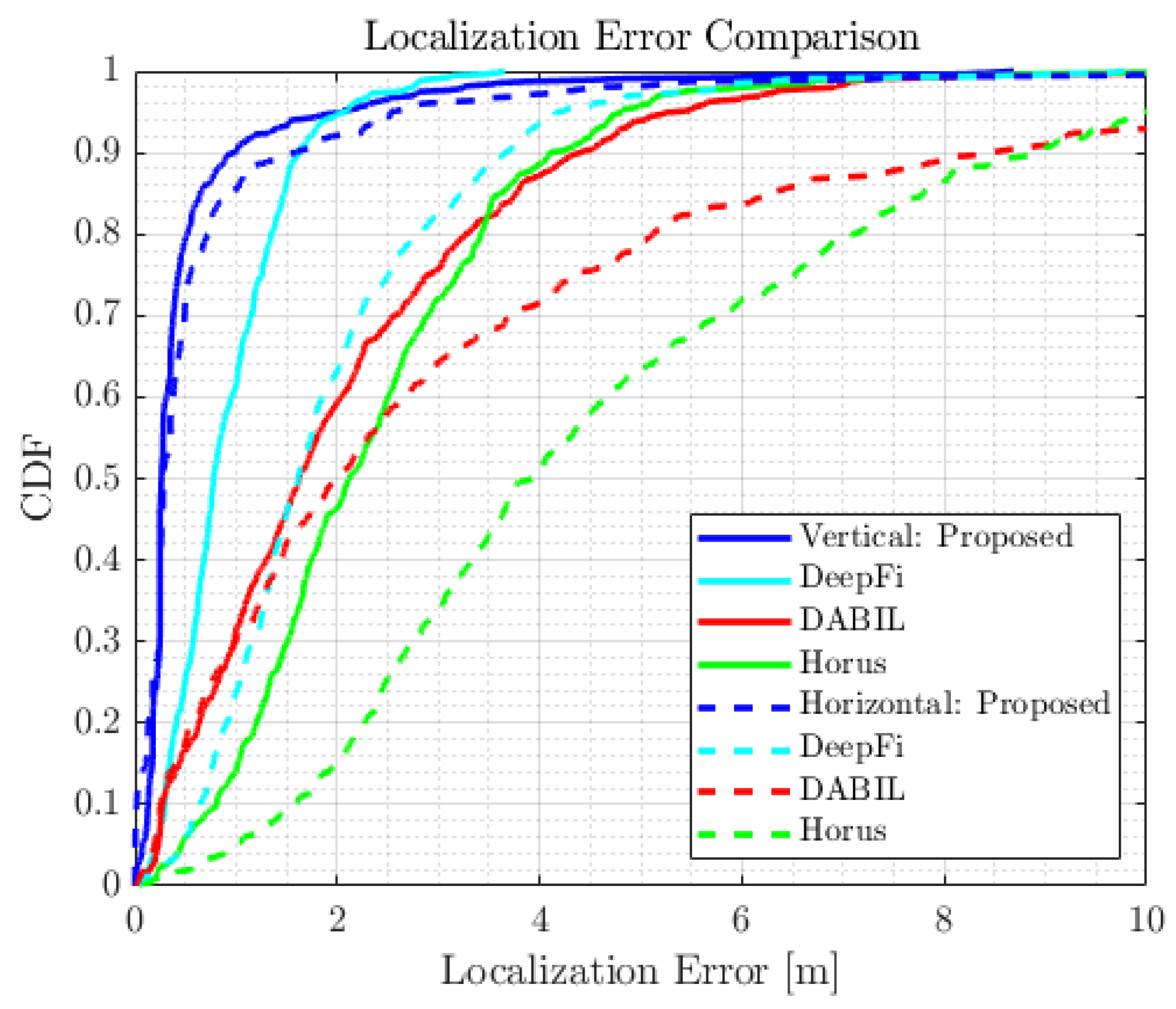
A depiction of the TDVS experimental configuration for the transmitter and receiver setup is shown in Figure 14 along with the depiction of the associated hardware front-end and cascaded SDR when located in the cluttered hardware room. A low noise amplifier and centered 915 MHz bandpass filter spanning 30 MHz was used for all three channels of the TDVS receiver prior to the sampling by the X310 SDR. The transmitter was designed as a half-wave dipole for 915 MHz frequency operation, while also allowing the flexibility to evaluate polarization impacts on the designed localization procedure (similar to that evaluated in the simulation model). On the transmit control side, a repeated 5 MHz beacon BPSK sequence was generated by the M8190A AWG designed by Keysight Technologies. On the receiver side, the TDVS sensed the transmitted BPSK sequence in three orthogonal dimensions, which was then followed by three low noise amplifiers and bandpass filters for signal conditioning. The final output was then passed to the X310 for approximately a 1 s duration collects resulting in a realization of 500 received beacon packets. Using the received BPSK beacon information at all locations, a PkNN and DAE based PkNN was constructed on all six datasets (i.e., three locations and two polarizations) where the results of the localization are depicted in CDF form in Figure 15.
The results portrayed by Figure 15 demonstrate consistent results found in the simulated model. In the simulation, Office #2 offered the best performance in localization of vertically polarized transmitters, which was consistent with the experiment. Considering the horizontal case, it was evident that the hardware area outperformed the other two rooms, which deviated from the simulation predictions. From the experimental statistics, there was an increase in the standard deviation between the horizontal and vertical polarization states of the transmitter. This implies that the scattering information within the CSI had higher fluctuation in horizontally polarized emitters. Such fluctuations imply that the prediction of optimum location for receiver placement in the proposed localization system requires extensive modeling in the simulation domain that considers all forms of clutter that could exist in the experimental setting. The simulation model had, however, predicted the best average performance to be for vertically polarized transmitters, consistent with the experimental evidence.
Due to the high presence of interference, the DAE worked optimally to obtain high localization precision when compared to the traditional TDVS approach, which did not employ deep learning for training PkNN. The designed two layer DAE was trained with 75 neurons on the first layer and 25 on the second with an interference duration of 50% and potential power levels of 5, 10, and 30 dB, at a minimum distance of 30 m away. The specific parameters were defined based on experimentally measured power levels in the RF environment. Comparing the horizontal and vertical transmitter polarization cases, it was apparent that high variability can be found in the designed localization algorithms if the polarization of the transmitter and receiver was not accounted for in the algorithmic designs. A higher level statistical analysis of the aforementioned experimental results can be found in Table 3.
6. Conclusions
The first demonstration of the TDVS for use in finite localization in indoor environments on an SDR platform was introduced. The design and implementation of a probabilistic deep learning model based on acquired 3D CSI showed resilience to interference, while also performing better than other literature based algorithms that employed various receivers in the localization process. Simulation and experimental results demonstrated the importance of having polarization diversity (or necessity to consider polarization) when attempting to develop localization algorithms for complex indoor environments. The results enlightened the importance of receiver placement and the fluctuations in localization performance that can be realized for single receiver systems if not chosen properly. This document demonstrated the first SDR based localization system that can localize transmitters with sub-2 m error when employing a single TDVS and extracted 3D CSI from wireless transmitter beacons. The demonstration ensures that TDVS based technologies can offer improvements in CSI based algorithms as 3D scattering characteristics can be extracted and exploited in a probabilistic manner for enhanced accuracy in indoor localization.
Author Contributions
D.L.H. performed the simulations and the experiments, developed the algorithms, and wrote the first draft of the paper; R.M.N. supervised the research; D.M.J. provided assistance with algorithm development and analysis; all authors participated in refining the paper.
Funding
This research received no external funding.
Conflicts of Interest
The authors declare no conflict of interest.
Abbreviations
The following abbreviations are used in this manuscript:
| AP | Access point |
| AWG | Arbitrary waveform generator |
| BPSK | Binary phase shift keying |
| CSI | Channel state information |
| DAE | Denoising autoencoder |
| DoA | Direction of arrival |
| GMM | Gaussian mixture model |
| IPS | Indoor positioning system |
| LoS | Line-of-sight |
| NIC | Network interface card |
| NLoS | Non-line-of-sight |
| PkNN | Probabilistic k nearest neighbor |
| RF | Radio frequency |
| RSS | Received signal strength |
| SDR | Software defined radio |
| TDVS | Triad dipole vector sensor |
| WLAN | Wireless local access network |
References
- Roos, T.; Myllymäki, P.; Tirri, H.; Misikangas, P.; Sievänen, J. A Probabilistic Approach to WLAN User Location Estimation. Int. J. Wirel. Inf. Netw. 2002, 9, 155–164. [Google Scholar] [CrossRef]
- Bulten, W.; Rossum, A.C.V.; Haselager, W.F.G. Human SLAM, Indoor Localisation of Devices and Users. In Proceedings of the 2016 IEEE First International Conference on Internet-of-Things Design and Implementation (IoTDI), Berlin, Germany, 4–8 April 2016; pp. 211–222. [Google Scholar] [CrossRef]
- Youssef, M.; Agrawala, A.K. The Horus WLAN location determination system. In Proceedings of the 3rd International Conference on Mobile Systems, Applications, and Services (MobiSys), Seattle, WA, USA, 6–8 June 2005. [Google Scholar]
- Khatab, Z.E.; Hajihoseini, A.; Ghorashi, S.A. A Fingerprint Method for Indoor Localization Using Autoencoder Based Deep Extreme Learning Machine. IEEE Sens. Lett. 2018, 2, 1–4. [Google Scholar] [CrossRef]
- Xiao, C.; Yang, D.; Chen, Z.; Tan, G. 3-D BLE Indoor Localization Based on Denoising Autoencoder. IEEE Access 2017, 5, 12751–12760. [Google Scholar] [CrossRef]
- Wu, K.; Xiao, J.; Yi, Y.; Chen, D.; Luo, X.; Ni, L.M. CSI-Based Indoor Localization. IEEE Trans. Parallel Distrib. Syst. 2013, 24, 1300–1309. [Google Scholar] [CrossRef]
- Yazdanian, P.; Pourahmadi, V. DeepPos: Deep Supervised Autoencoder Network for CSI Based Indoor Localization. arXiv 2018, arXiv:1811.12182. [Google Scholar]
- Wu, G.; Tseng, P. A Deep Neural Network-Based Indoor Positioning Method using Channel State Information. In Proceedings of the 2018 International Conference on Computing, Networking and Communications (ICNC), Maui, HI, USA, 5–8 March 2018; pp. 290–294. [Google Scholar] [CrossRef]
- Wang, X.; Gao, L.; Mao, S.; Pandey, S. DeepFi: Deep learning for indoor fingerprinting using channel state information. In Proceedings of the 2015 IEEE Wireless Communications and Networking Conference (WCNC), New Orleans, LA, USA, 9–12 March 2015; pp. 1666–1671. [Google Scholar] [CrossRef]
- Wang, X.; Gao, L.; Mao, S. CSI Phase Fingerprinting for Indoor Localization With a Deep Learning Approach. IEEE Internet Things J. 2016, 3, 1113–1123. [Google Scholar] [CrossRef]
- Nambiar, V.; Vattapparamban, E.; Yurekli, A.I.; Güvenç, İ; Mozaffari, M.; Saad, W. SDR based indoor localization using ambient WiFi and GSM signals. In Proceedings of the 2017 International Conference on Computing, Networking and Communications (ICNC), Santa Clara, CA, USA, 26–29 January 2017; pp. 952–957. [Google Scholar] [CrossRef]
- Schmidt, E.; Inupakutika, D.; Mundlamuri, R.; Akopian, D. SDR-Fi: Deep-learning-based Indoor Positioning via Software-defined Radio. IEEE Access 2019, 7, 145784–145797. [Google Scholar] [CrossRef]
- Xie, T.; Zhang, C.; Wang, Z. WiFi TDoA indoor localization system based on SDR platform. In Proceedings of the 2017 IEEE International Symposium on Consumer Electronics (ISCE), Kuala Lumpur, Malaysia, 14–15 November 2017; pp. 82–83. [Google Scholar] [CrossRef]
- Vasudeva, K.; Çiftler, B.S.; Altamar, A.; Guvenc, I. An experimental study on RSS-based wireless localization with software defined radio. In Proceedings of the WAMICON 2014, Tampa, FL, USA, 6 June 2014; pp. 1–6. [Google Scholar] [CrossRef]
- Hall, D.L.; Narayanan, R.M.; Lenzing, E.H.; Jenkins, D.M. Passive Vector Sensing for Non-Cooperative Emitter Localization in Indoor Environments. Electronics 2018, 7, 442. [Google Scholar] [CrossRef]
- Hall, D.L.; Narayanan, R.M.; Jenkins, D.M.; Lenzing, E.H. Non-cooperative emitter classification and localization with vector sensing and machine learning in indoor environments. In Radar Sensor Technology XXIII; Ranney, K.I., Doerry, A., Eds.; International Society for Optics and Photonics: Bellingham, WA, USA, 2019; Volume 11003, pp. 280–293. [Google Scholar] [CrossRef]
- Daldorff, L.K.S.; Turaga, D.S.; Verscheure, O.; Biem, A. Direction of Arrival estimation using single tripole radio antenna. In Proceedings of the 2009 IEEE International Conference on Acoustics, Speech and Signal Processing, Taipei, Taiwan, 19–24 April 2009; pp. 2149–2152. [Google Scholar] [CrossRef]
- Chen, L.; Aminaei, A.; Falcke, H.; Gurvits, L. Optimized estimation of the Direction of Arrival with single tripole antenna. In Proceedings of the 2010 Loughborough Antennas Propagation Conference, Loughborough, UK, 8–9 November 2010; pp. 93–96. [Google Scholar] [CrossRef]
- Compton, R. The tripole antenna: An adaptive array with full polarization flexibility. IEEE Trans. Antennas Propag. 1981, 29, 944–952. [Google Scholar] [CrossRef]
- Durgin, G. Space-Time Wireless Channels, 1st ed.; Prentice Hall Press: Upper Saddle River, NJ, USA, 2002. [Google Scholar]
- Vincent, P.; Larochelle, H.; Lajoie, I.; Bengio, Y.; Manzagol, P.A. Stacked Denoising Autoencoders: Learning Useful Representations in a Deep Network with a Local Denoising Criterion. J. Mach. Learn. Res. 2010, 11, 3371–3408. [Google Scholar]
- Baldi, P.; Hornik, K. Neural Networks and Principal Component Analysis: Learning from Examples Without Local Minima. Neural Netw. 1989, 2, 53–58. [Google Scholar] [CrossRef]
- Vlasenko, I.; Nikolaidis, I.; Stroulia, E. The Smart-Condo: Optimizing Sensor Placement for Indoor Localization. IEEE Trans. Syst. Man Cybern. Syst. 2015, 45, 436–453. [Google Scholar] [CrossRef]
- Perez-Vega, C.; Zamanillo, J.M. Path-loss model for broadcasting applications and outdoor communication systems in the VHF and UHF bands. IEEE Trans. Broadcast. 2002, 48, 91–96. [Google Scholar] [CrossRef]
Figure 1.
Denoising autoencoder architecture with corrupted 3D CSI as the feature vector input.

Figure 2.
Depiction of the training process for the hidden layers of the denoising autoencoder on the input 3D CSI feature vectors for the first two stages. (a) Hidden Layer #1 (b) Hidden Layer #2.
Figure 2.
Depiction of the training process for the hidden layers of the denoising autoencoder on the input 3D CSI feature vectors for the first two stages. (a) Hidden Layer #1 (b) Hidden Layer #2.

Figure 3.
Simulated indoor environment used to evaluate IPS algorithms in the literature and compare to the proposed 3D CSI approach.
Figure 3.
Simulated indoor environment used to evaluate IPS algorithms in the literature and compare to the proposed 3D CSI approach.

Figure 4.
Evaluating 3D CSI relationship between spatial separation of training points in the indoor environment and distance of all training points as a function of space and the conditional probability of the PkNN. (a) distance between all training points. (b) Conditional probability relationship between scaling parameter and distance.

Figure 5.
Localization performance of the proposed 3D CSI method when placing a TDVS receiver in each room of the simulated indoor environment for (a) vertical transmitter polarization and (b) horizontal transmitter polarization.
Figure 5.
Localization performance of the proposed 3D CSI method when placing a TDVS receiver in each room of the simulated indoor environment for (a) vertical transmitter polarization and (b) horizontal transmitter polarization.

Figure 6.
Localization comparison between the proposed 3D CSI approach with other approaches prescribed in the IPS literature.
Figure 6.
Localization comparison between the proposed 3D CSI approach with other approaches prescribed in the IPS literature.

Figure 7.
Localization performance of 3D CSI and 3D CSI with deep learning DAE for a single receiver located in Office #2 for (a) vertical transmitter polarization and (b) horizontal transmitter polarization.
Figure 7.
Localization performance of 3D CSI and 3D CSI with deep learning DAE for a single receiver located in Office #2 for (a) vertical transmitter polarization and (b) horizontal transmitter polarization.

Figure 8.
Error surface of the localization algorithms for increased interference distances and corruption times and the simultaneous effect on 3D CSI extraction of a vertically polarized target emitter with interference power levels of (a) 7 dBm 3D CSI, (b) 13 dBm 3D CSI, (c) 7 dBm DAE 3D CSI, and (d) 13 dBm DAE 3D CSI.

Figure 9.
Error surface of the localization algorithms for increased interference distances and corruption times and the simultaneous effect on 3D CSI extraction of a horizontally polarized target emitter with interference power levels of (a) 7 dBm 3D CSI, (b) 13 dBm 3D CSI, (c) 7 dBm DAE 3D CSI, and (d) 13 dBm DAE 3D CSI.

Figure 10.
Average localization error as a function of increased interference power for the proposed 3D CSI and deep learning based 3D CSI methods.
Figure 10.
Average localization error as a function of increased interference power for the proposed 3D CSI and deep learning based 3D CSI methods.

Figure 11.
Channel equalization results for various known BPSK beacon preambles for NLoS Rayleigh distributed channel models: (a) LTE-ETU and (b) WLAN ETSI Model E.
Figure 11.
Channel equalization results for various known BPSK beacon preambles for NLoS Rayleigh distributed channel models: (a) LTE-ETU and (b) WLAN ETSI Model E.

Figure 12.
Doppler impact on channel estimation for: (a) the theory and (b) experimental measurements.
Figure 12.
Doppler impact on channel estimation for: (a) the theory and (b) experimental measurements.

Figure 13.
Experimental indoor laboratory environment used to test the indoor localization system and X310 SDR platform.
Figure 13.
Experimental indoor laboratory environment used to test the indoor localization system and X310 SDR platform.

Figure 14.
Experimental configuration in hardware area with (a) the hardware configuration and (b) signal conditioning of the SDR front-end.
Figure 14.
Experimental configuration in hardware area with (a) the hardware configuration and (b) signal conditioning of the SDR front-end.

Figure 15.
CDF localization performance for the TDVS and TDVS-DAE based algorithms for (a) vertical transmitter polarization and (b) horizontal transmitter polarization.
Figure 15.
CDF localization performance for the TDVS and TDVS-DAE based algorithms for (a) vertical transmitter polarization and (b) horizontal transmitter polarization.


Table 1.
Localization performances of various TDVS antenna placements.
| Vertical Polarization | Horizontal Polarization | |||
|---|---|---|---|---|
| Room Location | (m) | (m) | (m) | (m) |
| Corridor | 1.251 | 2.454 | 0.762 | 1.217 |
| Hallway | 1.556 | 3.323 | 1.607 | 2.780 |
| Hardware | 0.693 | 1.462 | 1.687 | 3.283 |
| Office 1 | 0.643 | 1.066 | 0.703 | 1.335 |
| Office 2 | 0.528 | 0.910 | 0.694 | 0.935 |
| Office 3 | 1.242 | 2.908 | 0.683 | 1.315 |
| Office 4 | 0.893 | 1.847 | 0.823 | 1.398 |
| Storage | 0.600 | 0.921 | 1.943 | 3.319 |
Table 2.
Localization Performances of Different IPS Algorithms.
| Vertical Polarization | Horizontal Polarization | |||
|---|---|---|---|---|
| Algorithm | (m) | (m) | (m) | (m) |
| 3D CSI | 0.528 | 0.910 | 0.694 | 0.935 |
| DeepFi | 0.924 | 0.597 | 1.946 | 1.365 |
| DABIL | 2.071 | 1.717 | 3.220 | 3.427 |
| Horus | 2.368 | 1.463 | 4.662 | 2.921 |
Table 3.
Localization performances of the experiment.
| Vertical Polarization | Horizontal Polarization | |||
|---|---|---|---|---|
| Room: Approach | (m) | (m) | (m) | (m) |
| Hardware: TDVS | 5.175 | 3.068 | 5.014 | 3.323 |
| Hardware: TDVS-DAE | 1.861 | 1.101 | 1.397 | 0.757 |
| Office 2: TDVS | 4.938 | 3.375 | 5.211 | 3.336 |
| Office 2: TDVS-DAE | 1.760 | 0.834 | 2.621 | 1.219 |
| Office 3: TDVS | 5.533 | 3.476 | 5.488 | 3.183 |
| Office 3: TDVS-DAE | 2.230 | 1.083 | 2.417 | 1.350 |
© 2019 by the authors. Licensee MDPI, Basel, Switzerland. This article is an open access article distributed under the terms and conditions of the Creative Commons Attribution (CC BY) license (http://creativecommons.org/licenses/by/4.0/).
Share and Cite
MDPI and ACS Style
Hall, D.L.; Narayanan, R.M.; Jenkins, D.M. SDR Based Indoor Beacon Localization Using 3D Probabilistic Multipath Exploitation and Deep Learning. Electronics 2019, 8, 1323. https://doi.org/10.3390/electronics8111323
AMA Style
Hall DL, Narayanan RM, Jenkins DM. SDR Based Indoor Beacon Localization Using 3D Probabilistic Multipath Exploitation and Deep Learning. Electronics. 2019; 8(11):1323. https://doi.org/10.3390/electronics8111323
Chicago/Turabian StyleHall, Donald L., Ram M. Narayanan, and David M. Jenkins. 2019. "SDR Based Indoor Beacon Localization Using 3D Probabilistic Multipath Exploitation and Deep Learning" Electronics 8, no. 11: 1323. https://doi.org/10.3390/electronics8111323
Note that from the first issue of 2016, this journal uses article numbers instead of page numbers. See further details here.