Influence of Power Modules on the Thermal Design of Laminated Busbars

Abstract

The temperature of laminated busbars has to be limited to prevent their inner electrical insulators from over-heating. In that purpose, Finite Elements Method (FEM) simulations are usually conducted to evaluate the busbar's temperature. However, the thermal influence of external heat sources such as power modules has to be considered to obtain an accurate temperature repartition estimation. In this paper, the thermal influence of power modules on busbar temperature is first evaluated through simulation and experimental works. Then, a method based on the use of electrical equivalent circuits as boundary conditions is proposed to consider this issue and reduce the computation time.

1. Introduction

Laminated busbars are used in power electronics structures to reduce over-voltages across power devices during switching. They are generally composed of several conductive layers (copper, aluminum) separated by an insulating material enabling a reduction of stray inductances between DC-link capacitors and power modules. The estimation of laminated busbars stray inductances has been a subject of intense researches during the last two decades [1,2]. It is now possible to optimize their shape to reduce stray inductances and have a satisfying current sharing between the different elements [3,4,5,6,7,8]. Two methods are mainly used: Finite Elements Method (FEM) to have accurate results and Partial Element Equivalent Circuit (PEEC) to reduce computation times and to allow for easier optimization process. On the other hand, the design of laminated busbars also faces thermal issues. Indeed, busbar temperature must be kept below a maximum value depending on the type of insulator. As an example, when using polyethylene terephthalate (PET), busbar temperature should not exceed 105 °C. Otherwise, electrical insulation between the different conductive layers cannot be guaranteed since over-heating may appear.

The temperature estimation of laminated busbars has to be made through two steps: first, an electrical and electromagnetic study is conducted to calculate the Joule losses generated in the system. Then, these losses are injected in the heat equation to estimate the temperature elevation. Since the electrical conductivity of conducting parts depends on temperature, a physical coupling between electrical and thermal calculations has to be carried out. This methodology is well mastered for busbars in power distribution systems because their geometries are relatively simple [9]. Analytical methods are thus largely employed [10,11,12]. In the case of laminated busbars, the current flow is generally complex involving the use of numerical tools. Gerlaud et al. [13] and Li et al. [14] propose to use commercial 3D FEM Multiphysics tools. Because calculation times can be significant using FEM, Smirnova et al. [15] propose to use lumped parameter thermal models to estimate the temperature inside a laminated busbar. Puigdellivol et al. [16] proposed a method to solve a 3D multilayer busbar problem using 2D FEM. With this solution, the computation time can be largely reduced.

The temperature of a laminated busbar depends on its self-heating due to Joule losses. This phenomenon is generally well studied in literature. Authors also take into account convective and radiative heat fluxes between busbars and their environment by introducing heat transfer coefficients [13,14,15,16]. However, the influence of heat conduction through the terminals of the busbar is often forgotten. Actually, the connections with power cables, DC-link capacitors and power modules can lead to non-negligible heat fluxes in the busbar resulting in inaccurate temperature estimations [17,18].

The aim of the present paper is to propose a methodology to take into account the influence of heat conduction between busbars and power modules during busbar thermal design. The first option is a complete electro-thermal modeling approach including the busbar, the power module and the heatsink. It is probably the most accurate solution, but the physical properties of all materials and the geometry of all elements have to be well known. Furthermore, a precise semiconductor loss model and a CFD (Computational Fluid Dynamic) tool are required to obtain a good evaluation of the power module base plate temperature which is an important parameter during the busbar design. This option is therefore time consuming and has a huge impact on the cost of the study. The second option which is largely proposed in literature is to simulate heat transfers in the busbar only. However, in these conditions, the thermal coupling is not taken into account. Thus, this paper will propose a new methodology which consists in a trade-off between calculation time and accuracy through the use of an electrical equivalent circuit thermal model of the power module terminal as a boundary condition for the 3D FEM modelling.

The paper will be organized as follows. Firstly, the devices under test and the simulation procedure will be described. Several experimental tests will then be presented to validate the simulation results and confirm the thermal modelling approach. Finally, the proposed methodology will be presented and the accuracy of the results will be compared with a state of the art busbar design procedures.

2. Materials and Methods

2.1. Power Elements

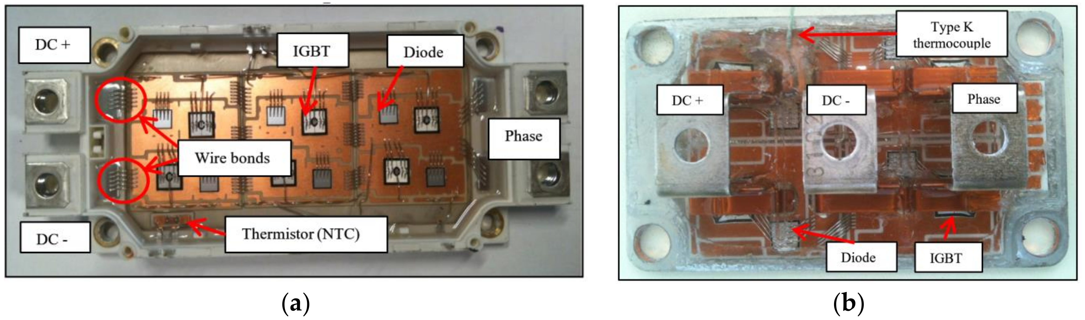
Since heat transfers in busbar/power module assemblies are dependent on power terminals technology [10], two different commercial power modules are chosen with different connection types representing what is mostly used today. The first one (Infineon—FF150R12ME3G—1200 V—150 A, Infineon, Neubiberg, Germany) includes an inverter phase leg using six IGBT—Insulated Gate Bipolar Transistor—and six diodes (three paralleled dies for each switch). As shown in Figure 1a, the power terminals are linked to the isolated substrate by wire bonding. This module includes a thermistor to measure the substrate temperature in operating conditions and will be called “Module M” in the following sections. The second module (Figure 1b) (Infineon—FF150R12KE3G—1200 V—150 A, Infineon, Neubiberg, Germany) includes an inverter phase leg using four diodes and four IGBT (2 paralleled dies for each switch). The power terminals are directly soldered onto the metallization. This module will be called “Module K”.

A busbar (Figure 2) has been designed and fabricated by Mersen Company using standard fabrication techniques. It has a 10 × 10 cm square shape and is made of two copper layers (thickness 0.8 mm) separated by a 0.23 mm thick PET layer. The whole external busbar area (except the connections) is covered by a 0.15 mm thick PET layer. It was designed to be connected either to module K or to module M.

2.2. System Modelling Using Comsol Multiphysics

2.2.1. Geometry and Physical Properties

The Comsol Multiphysics software has been chosen since it is well adapted for solving problems including coupling between different physical phenomena. The used software modules are: “AC/DC module” to solve the electrical conduction equation and “Heat Transfer module” to solve the heat equation in solids (convection and radiation heat transfers are only considered as boundary conditions is this study).

The geometrical construction of the busbar in the simulation software was easy because its dimensions were accurately known. On the contrary, concerning the power terminals, a partial disassembly of the power modules and a measurement of their respective dimensions were necessary. A precise estimation of the wire bonding diameter (500 µm) was also necessary because their internal dissipation is significant compared with other parts. Figure 3 presents the simulated geometries of power terminals. In this figure, the dark grey elements are not part of the power terminals; they represent the plastic in which the terminals are drowned.

Equations (1)–(4) give the expressions of the thermal and electrical conductivities of the conductive parts (copper for the busbar and bare parts of the power terminals, aluminum for wire bonding) [19]. Equation (5) gives the expression of the insulator thermal conductivity.

$${\sigma }_{Cu }\left(T\right)= \frac{1}{1.725·{10}^{-8}\left[1+3.93·{10}^{-3}\left(T-273.15\right)\right]}\left[\mathrm{S}/\mathrm{m}\right]$$

(1)

$${\mathsf{\lambda }}_{Cu }\left(T\right)=406.7-0.065\left(T-273.15\right)\left[\mathrm{W}/\left(\mathrm{m}·\mathrm{K}\right)\right]$$

(2)

$${\sigma }_{Al }\left(T\right)= \frac{1}{2.82·{10}^{-8}\left[1+3.91·{10}^{-3}\left(T-293.15\right)\right]}\left[\mathrm{S}/\mathrm{m}\right]$$

(3)

$${\mathsf{\lambda }}_{Al }=238 \left[\mathrm{W}/\left(\mathrm{m}·\mathrm{K}\right)\right]$$

(4)

$${\mathsf{\lambda }}_{PET }\left(T\right)=0.07+2.2·{10}^{-5}{\left(T-273.15\right)}^{1.873}\left[\mathrm{W}/\left(\mathrm{m}·\mathrm{K}\right)\right]$$

(5)

where σ_Cu and σ_Al are respectively the electrical conductivities of copper and aluminum. λ_Cu, λ_Al and λ_PET are the thermal conductivities of copper, aluminum and PET. T is the temperature in Kelvin.

2.2.2. Boundary Conditions

For this study, the frequency effects on the electrical resistance (skin effect) are not considered. It could be done to have a better estimation of Joule losses [15] but their impact is not critical for the present purpose. Indeed, the aim of this work is mainly to study the thermal coupling between busbars and power modules. However, for a complete busbar thermal design, it is generally necessary to take into account this physical phenomenon because it has a non-negligible influence on the current density repartition inside the busbar.

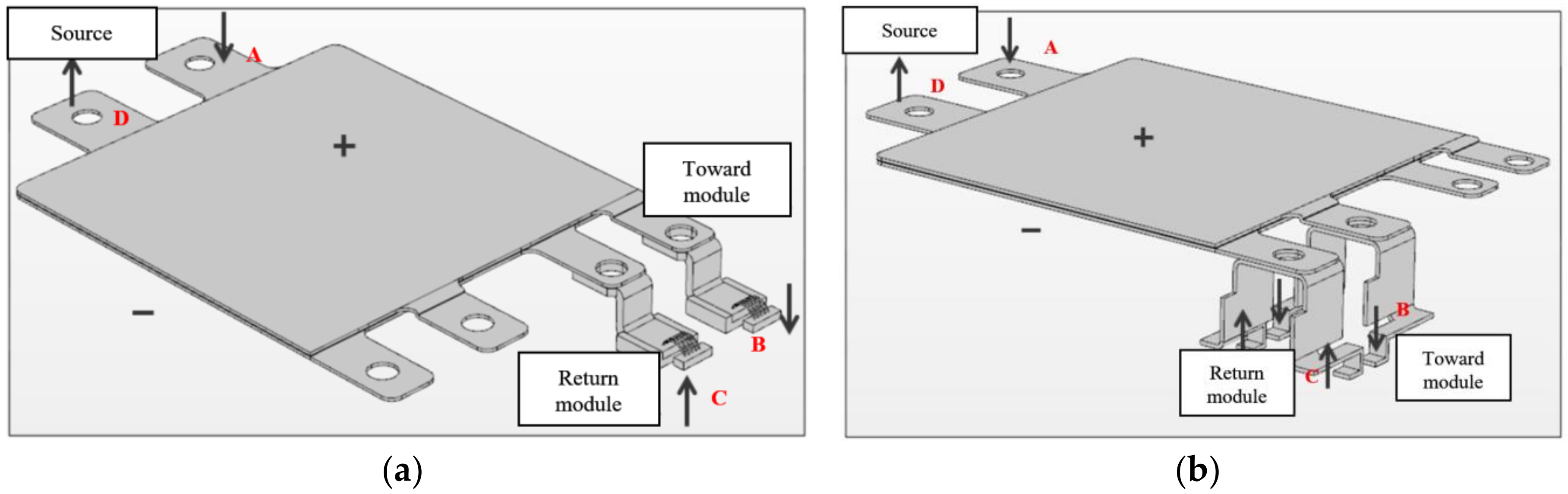
A direct current (representing the RMS—Root Mean Square—current in the DC electrodes) I_eff is injected in the top layer of the busbar (Figure 4—point A) and continues through the positive power terminal toward the module (point B). The current comes back through the negative power terminal (point C) and the bottom layer of the busbar to the negative power source terminal (point D). The electrical boundary conditions are applied on the dark areas shown in Figure 5 and the current density entering each surface is considered to be uniform. All other surfaces are insulated. To simplify the problem this figure presents the boundary conditions for a direct current of 150 A.

Free convection and radiation heat transfers are applied on the free surfaces of the busbar (all surfaces except those in contact with the power module). The radiation heat transfers are considered in the simulation by using the surface emissivity, the surface temperature, the ambient temperature and the view factors between surfaces. The convection heat transfers are studied using the Newton law and heat transfer coefficients are obtained by correlations provided in literature [20]. The main convection configurations are: horizontal surface with heat flux toward the top and horizontal surface with heat-flux toward the bottom. The related heat transfer coefficients h_c are given in

Table 1. Heat transfer coefficients for free convection on horizontal flat surfaces—ΔT is the difference between surface and ambient temperatures—L is a characteristic dimension of the surface [20].

Surface Orientation	Measurement	Unit
Horizontal heat source—Heat flux towards the top	$h_c=1.32 {\left(\frac{\Delta T}{L}\right)}^{0.25}$	W/(m²K)
Horizontal heat source—Heat flux towards the bottom	$h_c=0.59 {\left(\frac{\Delta T}{L}\right)}^{0.25}$	W/(m²K)

. According to each different materials and surface aspects, different emissivities have been applied: 0.3 for copper surfaces and 0.9 for PET ones. These values were estimated through infrared measurements.

In normal operating conditions, the heat dissipated and transferred by conduction in the busbar and the power terminals (several W) can be neglected compared to the total heat generated by the power semi-conductors (hundreds of W). That means that the heat transfer in the power terminals has not a strong influence on the temperature of the connection between them and the isolated substrate. This temperature is driven by the heat dissipation of semi-conductor dies and the heat sink efficiency, and not by other dissipations in the busbar and power terminals. Consequently, the problem can be described as heat conduction in semi-infinite environment (a perturbation on one side does not influence the other side) with a constant temperature as boundary condition. That is the reason why a temperature condition (T_bp) is applied on the contact surface between the power terminals and the isolated substrate metallization (dark areas in Figure 5). For the module M, the same temperature is applied on the contact surface between the plastic and the base-plate (bottom surface of dark element in Figure 3).

3. Results

3.1. Simulation Results

The simulation results presented in Figure 6 come from the model detailed before with the following input parameters: I_eff = 150 A, ambient temperature T_a = 25 °C and T_bp = 80 °C. To carry out a simulation that does not take into account heat transfers between the power terminals and the busbar (classical method), the latter has been first simulated alone as shown in Figure 6a. In this case the boundary conditions were modified: convection and radiation boundary heat transfers were affected on all surfaces. In these conditions, the maximum busbar temperature reached 46 °C. The same simulation has been done with the power terminals of the module M connected to the busbar as shown in Figure 6b. The maximum busbar temperature went up to 92 °C which corresponded to an increase of 46 °C (219% increase with ambient temperature as a reference). The same method was applied for the module K. Without taking into account heat transfers in power terminals, the busbar reached a maximum temperature of 45 °C. When considering the power terminals, the temperature rose to 72 °C, corresponding to a 140% increase.

With these first simulation results based on a specific case, it was confirmed that the role of power terminals could not be neglected if a precise thermal busbar design is needed. Even if some geometries exist where the role of power terminals is not so important, a study remains necessary to evaluate its real influence on the busbar temperature. Note that none of electrical and thermal contact resistances were considered in all simulations. In fact, they depend on lots of conditions: nature and roughness of the metal, coating, pressure. However, in the case of simple busbars, the electrical resistance was estimated to be lower than 20 µΩ for contact areas close to 1 cm² [21]. The thermal contact resistance was supposed to be lower than 0.5 K·W⁻¹ for the same area [22].

In order to confirm our modelling approach and our simulation results, several experimental setups were carried out. In the following paragraphs, thermal and electrical phenomena will be presented separately.

3.2. Experimental Results

3.2.1. Thermal Aspects

The setup shown in Figure 7 allowed us to determine the thermal resistance of the power terminals by measuring different temperatures and heat fluxes. Two modules of the same type were fixed together via their base-plates and were placed in an insulating box. One module was fed with a current (dissipating power module) in order to heat up (via the diodes) the other one (module under test). The dissipated power in this module was P₁. The power terminals of the module under test were linked to the heat sink via a brass plate (Figure 7b). The heat could flow either through the box envelope (P_env) or through the power terminals (P_pt). The electrical power P₁ injected in the module was calculated measuring current and voltage across the diodes. The thermal resistance R_env of the insulating box was first estimated without the heat sink and the brass plate (P_pt = 0) and measuring the power module base-plate and ambient temperatures (T_bp and T_a) (Equation 6). Knowing this thermal resistance, it was possible to estimate the power flowing through the envelope (P_env) when the heat sink was added. Thus, the heat flux going through the power terminals could be deduced (Equation (7)). Knowing this heat flux, the base-plate temperature (T_bp), and the power terminal temperature (T_pt), the thermal resistance R_pt of one power terminal was calculated by Equation (8).

$$R_{env}= \frac{T_{bp}-T_a}{P_{env}}[\mathrm{K}/\mathrm{W}]$$

(6)

$$P_{pt}= P_1-P_{env}\left[\mathrm{W}\right]$$

(7)

$$R_{pt}=2\frac{T_{bp}-T_{pt}}{P_{pt}}\left[\mathrm{W}\right]$$

(8)

Measurement results were compared to simulated ones in

Table 2. Comparison between measured and simulated results of power terminals thermal resistances R_pt. The error is defined by: (maximum value—minimum value)/(minimum value).

	Measurement	Simulation	Error
Module M	31 K/W	31.6 K/W	2%
Module K	7.2 K/W	7 K/W	3%

. They were very close to each other. From the thermal resistance point of view, the modelling approach seemed to be validated. It has to be noted that, because of the wire bonds, the thermal resistance of module M was five times higher than this of module K.

3.2.2. Electrical Aspects

Another experimental setup was built to measure the electrical resistances of the power terminals and the busbar in order to quantify the heat generation by Joule effect in these elements. Because of their very low resistance (few tens of μΩ), the tests were made under high current (several tens of A) to have accurate voltage measurements (few mV) using the HBM Gen3i (HBM France SAS, Mennecy, France)acquisition system and GN610 unit input boards (2MEch/s-18bits) (HBM France SAS, Mennecy, France). To limit the self-heating of the different elements during current injection, voltage measurements were carried out using short current pulses (<1 ms). In these conditions, it could be assumed that the voltage measurements were done at room temperature. The voltage across the different elements was measured using probe needles placed near the end of each element. The measured electrical resistances were compared to the simulated ones in

Table 3. Electrical resistance measurements and simulation. The error is defined by: (maximum value—minimum value)/(minimum value).

		Power Terminals	Busbar	Wire Bonding
Module M	Measurements	16.5 µΩ	79.2 µΩ	272 µΩ
	Simulations	19 µΩ	76.5 µΩ	277 µΩ
	Error	15%	3.5%	2%
Module K	Measurements	54.2 µΩ	61 µΩ	NA
	Simulations	54.9 µΩ	64.1 µΩ	NA
	Error	1.5%	5%	NA

. As seen in this table, the resistances of three elements were measured: power terminal, busbar and wire bonding for module M. For simulation results, the voltage probes were placed at the same locations than during the experimental tests. The temperature was uniform (electrical simulation only) and was the same than this measured during experimental tests. The error concerning power terminals of module M was more important than the others because of their difficult access. Indeed, they were drowned in the plastic so their exact shape was not known which could lead to a less accurate simulation results. For the other parts, the error was very low and validated the electrical simulations.

The aim of electrical resistance measurements was to determine the heat generated by Joule effect in each element. However the heat dissipation was not uniform because of higher current densities in specific locations, especially near contact areas. Therefore, there were large electrical potential variations in these areas compared to the others. A dissipation estimation only based on resistance measurements between two points was thus non accurate. In order to take in account these effects, the “contact” resistance between the power module and the busbar was also measured, the needles being placed at the same locations than during resistance measurements (Figure 8). This new resistance R_ca represented the participation of both the voltage variations near the contact area and the actual contact resistance. Thus Joule losses in each element were approximated by the following equation:

$$P_J=\left(R+\frac{R_{ca}}{2}\right)I_{eff}^2=R_e{I}_{eff}^2 \left[W\right]$$

(9)

where R is the resistance measured as presented in Table 3 and R_e the global resistance of the power terminal.

Table 4. Power dissipation P_J in the different elements—I_eff = 150 A. The error is defined by: (maximum value—minimum value)/(minimum value).

		Wire Bonds + Power Terminals	Busbar
Module M	Measurements	6.87 W	1.9 W
	Simulations	6.98 W	1.85 W
	Error	1.5%	2.5%
Module K	Measurements	1.15 W	1.3 W
	Simulations	1.15 W	1.41 W
	Error	0%	7%

compared the Joule losses estimated using Comsol and using Equation (9). It showed that if the resistance near the contact area was measured and added to the elementary resistance from Table 3, the total heat generated by Joule effect was accurately calculated.

3.2.3. Global System

In a last setup, the power module and the busbar were fixed together and the module was cooled by a forced convection heat sink. The system was fed in direct current circulating through the diodes of the power module and the temperature was measured in different locations with K type thermocouples (Figure 9). These temperatures were compared with simulation results in

Table 5. Power dissipation P_J in the different elements—I_eff = 150 A–T_a = 26.5 °C—The error calculation is made using T_a as reference temperature. The error is defined by: (maximum value—minimum value)/(minimum value—ambient temperature).

		T1	T2	T3	T4	Tc-	Tc+
Module M	Measurements	44.2 °C	42.6 °C	48.1 °C	43 °C	62.4 °C	66.7 °C
	Simulations	43.8 °C	43.5 °C	49.8 °C	45.5 °C	65.4 °C	68.7 °C
	Error	2%	5%	8%	15%	8%	5%
Module K	Measurements	47.6 °C	48.3 °C	48.9 °C	51.5 °C	59.2 °C	58 °C
	Simulations	48.5 °C	49.2 °C	50 °C	53.3 °C	62.8 °C	61.2 °C
	Error	4%	4%	5%	7%	9%	10%

. The ambient temperature T_a and the current were measured to be entered as boundary conditions of the simulation works. It has to be noted that the temperatures of the electrical connections between the busbar and the power source (T_bb− and T_bb+) were dependent on the global electro-thermal modeling of the power source. In a same manner, the base plate temperature of the power module depended on the effectiveness of the heat sink. Therefore, temperatures T_bb+, T_bb− and T_bp were also measured and entered as boundary conditions. It allowed us to constrain the simulation domain to the busbar and the power terminals elements only. As shown in Table 5, the estimated temperatures were very close to the measured ones with a maximum error of 15%. The main deviation could be due to differences in convective and radiative heat transfers between simulations and experiments.

4. Discussion

Based on the previous experimental validation of the simulation works, this section proposes a discussion about the thermal modelling approach that has to be carried out during the busbar design. Both power modules will be treated separately due to their different inner structures.

4.1. Power Terminals with a Solder Attach

For power modules with a construction which is close to Module K, each power terminal is attached to the insulating substrate via a soldering process. It can thus be seen as a copper bar with a thermal resistance R_pt and an electrical resistance R_e. These resistances can be respectively measured using setups presented in the previous section. An equivalent thermal circuit can then be implemented as presented in Figure 10. In this model, the total thermal resistance of the bar is R_pt and the total Joule losses are P_J1 + P_J2. It is assumed that the section of the copper plate is uniform (which is not really the case for module K—Figure 3). In Figure 10, the Joule losses depend on copper temperature and can be approximated by:

$$P_{J1}= R_e\left(T_a\right)\left[1+{\alpha }_{Cu}\left(\frac{T_c+T_{pt1}}{2}-T_a\right)\right]I_{eff}{}^2\left[\mathrm{W}\right]$$

(10)

$$P_{J2}= R_e\left(T_a\right)\left[1+{\alpha }_{Cu}\left(\frac{T_{bp}+T_{pt2}}{2}-T_a\right)\right]I_{eff}{}^2\left[W\right]$$

(11)

where R_e (T_a) is the electrical resistance of the power terminal measured at ambient temperature and α_Cu = 0.00393 is the temperature coefficient of the copper resistivity. The other parameters of Equations (10) and (11) are presented in Figure 10.

The thermal model presented in Figure 10 can be used as a boundary condition of the busbar simulation. To verify this statement, the heat flux flowing from the power terminal to the busbar (Ф_circuit) was calculated as a function of T_c using the equivalent thermal circuit. Then the busbar only was simulated using Comsol. A temperature condition T_c was affected on surfaces which were located at power module / busbar electrical connections interfaces. The heat flux Ф_Comsol entering the busbar from the contact area was calculated for several T_c values. The T_c value which has to be affected in the Comsol simulation can then be determined by using the heat flux conservation law.

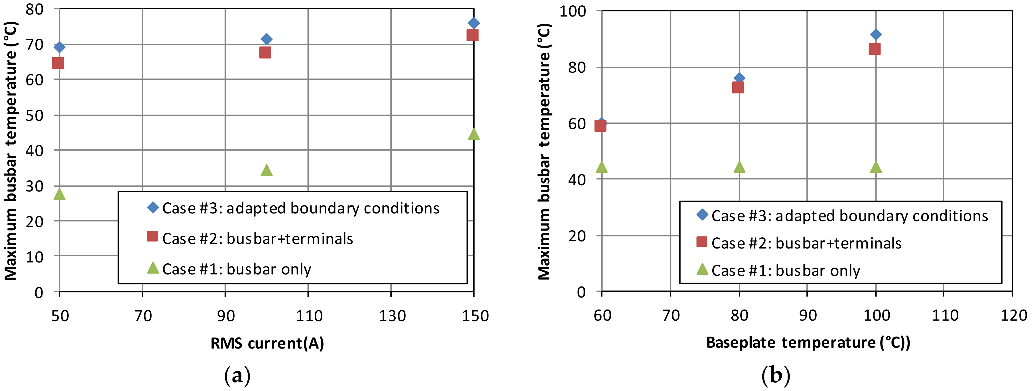
Finally, the maximum busbar temperature was calculated using three different methods:

• Case #1: simulation of the busbar only without taking into account the thermal influence of the power module,
• Case #2: simulation of the busbar and the power terminals,
• Case #3: simulation of the busbar only implementing the thermal circuit as boundary conditions.

The results are compared in Figure 11. Figure 11a shows the variation of the maximum busbar temperature for different RMS currents I_eff and Figure 11b for several base-plate temperatures T_bp. Using case #2 as a reference, it is clear that the simulations of the busbar only give large estimation errors. On the other hand, the use of the new boundary condition gives results which are very close with a maximum difference of 12%. This difference can be explained by the different assumptions which were made during the thermal circuit construction and particularly the section of the power terminal which was assumed to be uniform.

4.2. Power Terminals with a Wire Bonding Attach

The physical construction of module M implies that the thermal and electrical resistances of the power terminals are divided in two separate parts: bond wires made in aluminum and a copper bar. Therefore the use of a thermal model as presented in Figure 10 seems to be not suitable. However, Table 3 shows that both electrical and thermal resistances of the copper bar are significantly lower than these of the bond wires. As a first approximation, the thermal modeling can thus be made using the electrical circuit presented in Figure 10 with:

$$P_{J1}= R_e\left(T_a\right)\left[1+{\alpha }_{Al}\left(\frac{T_c+T_{pt1}}{2}-T_a\right)\right]I_{eff}{}^2\left[\mathrm{W}\right]$$

(12)

$$P_{J2}= R_e\left(T_a\right)\left[1+{\alpha }_{Al}\left(\frac{T_{bp}+T_{pt2}}{2}-T_a\right)\right]I_{eff}{}^2\left[W\right]$$

(13)

where α_Al = 0.00391 is the temperature coefficient of aluminum.

Figure 12a shows the evolution of the maximum busbar temperature for cases #1 to #3 as a function of the baseplate temperature for module M. The difference between case #2 and #3 is in the range 20 to 23%. It is higher than for module K which is due to a too simple thermal modeling. In Figure 12b, a more representative thermal circuit is presented. It was constructed thanks to complementary temperature measurements during the tests. These measurements permitted to determine the thermal resistance R_pt,Cu and R_pt,Al of both copper and aluminum parts respectively. R_pl is the thermal resistance of the plastic element between the copper bar and the baseplate (dark grey element in Figure 3). It was estimated to be 70 K·W⁻¹ measuring its thickness and considering that its thermal conductivity was 0.15 W.m⁻¹.K⁻¹. The maximum busbar temperature was estimated using this thermal circuit as boundary condition. The results are presented in Figure 12a (case #3b). The modelling approach is better with a temperature difference lower than 13% compared to case #2 but the thermal characterization is more complex.

5. Conclusions

As already claimed by different authors [17,18], this paper confirms that the thermal influence of power modules on busbar temperature can be significant. Large temperature underestimations can thus be done if only the busbar is simulated during the design, which could affect its lifetime. It was demonstrated that these underestimations could reach approximately 100 °C in worst cases, especially when the power module includes wire-bonding electrical connections.

The best solution to have accurate temperature estimations is to conduct global simulations of busbars, power modules and heat sinks (

Table 6. Comparison of different modelling techniques.

Solution	Advantages	Drawbacks
Global simulations of busbars, power modules and heat sinks	Can be accurate	Very time consuming, knowledge of a large number of data: geometries and physical properties
Simulation of the busbar and the power terminals	Can be accurate	The base plate temperature has to be measured, the geometry and physical properties of the power terminal must to be known
Simulation of the busbar only with adapted boundary conditions (proposed method)	Can be relatively accurate, relatively fast simulation procedure	Preliminary measurements have to be carried out: base plate temperature, thermal model of the power terminals
Simulation of the busbar only	Fast simulation procedure	Can be inaccurate

). Since this procedure is very time consuming, this paper presented a new methodology based on the simplification of the simulation work needing previous experimental procedures to be carried out. First, to reduce the computation time, it is proposed to only simulate busbars and power terminals. In this case, good description of power terminals and knowledge of the base plate temperature are required. Another proposition is to construct a thermal circuit of the power terminals from experimental tests and to use it as boundary conditions. By largely reducing the computation time, this method gives results which are very close to those obtained by simulating the power terminals of the power module (temperature difference lower than 10 °C). Furthermore, if this method were to be widely used, the power modules manufacturers could give the different parameters of the thermal circuit in their datasheets which would be helpful for busbar thermal designers.

References

- Chen, C.; Pei, X.; Chen, Y.; Kang, Y. Investigation, Evaluation, and Optimization of Stray Inductance in Laminated Busbar. IEEE Trans. Power Electron. 2013, 29, 3679–3693. [Google Scholar] [CrossRef]
- Pasterczyk, R.J.; Martin, C.; Guichon, J.M.; Schanen, J.L. Planar busbar optimization regarding current sharing and stray inductance minimization. In Proceedings of the 2005 European Conference on Power Electronics and Applications, Dresden, Germany, 11–14 September 2005. [Google Scholar]
- Mehrabadi, N.R.; Cvetkovic, I.; Wang, J.; Burgos, R.; Boroyevich, D. Busbar design for SiC-based H-bridge PEBB using 1.7 kV, 400 a SiC MOSFETs operating at 100 kHz. In Proceedings of the 2016 IEEE Energy Conversion Congress and Exposition (ECCE), Milwaukee, WI, USA, 18–22 September 2016. [Google Scholar]
- Tiwari, S.; Midtgard, O.-M.; Undeland, T.M. Design of low inductive busbar for fast switching SiC modules verified by 3D FEM calculations and laboratory measurements. In Proceedings of the 2016 IEEE 17th Workshop on Control and Modeling for Power Electronics (COMPEL), Trondheim, Norway, 27–30 June 2016. [Google Scholar]
- Wang, J.; Shen, Z.; Cvetkovic, L.; Mehrabadi, N.R.; Marzoughi, A.; Ohn, S.; Yu, J.; Xu, Y.; Burgos, R.; Boroyevich, D. Power Electronics Building Block (PEBB) design based on 1.7 kV SiC MOSFET modules. In Proceedings of the 2017 IEEE Electric Ship Technologies Symposium (ESTS), Arlington, VA, USA, 14–17 August 2017. [Google Scholar]
- Matallana, A.; Andreu, J.; Ignacio Garate, J.; Aretxabaleta, I.; Kortabarria, I. Analysis and Design of a Multilayer DC Bus With Low Stray Impedance and Homogenous Current Distribution. In Proceedings of the PCIM Europe 2018; International Exhibition and Conference for Power Electronics, Intelligent Motion, Renewable Energy and Energy Management, Nuremberg, Germany, 5–7 June 2018. [Google Scholar]
- Lin, X.; Li, J.; Johnson, C.M. Impedance analysis in a co-planar power bus interconnect prototype for low inductance switching. In Proceedings of the CIPS 2018; 10th International Conference on Integrated Power Electronics Systems, Stuttgart, Germany, 20–22 March 2018. [Google Scholar]
- Callegaro, A.D.; Guo, J.; Eull, M.; Danen, M.; Gibson, J.; Preindl, M.; Bilgin, B.; Emadi, A. Bus Bar Design for High-Power Inverters. IEEE Trans. Power Electron. 2018, 33, 2354–2367. [Google Scholar] [CrossRef]
- Grandvuillemin, J.; Chamagne, D.; Tiraby, C.; Glises, R. Ampacity of power bus bars for hybrid-electric or electric vehicles. In Proceedings of the 2008 IEEE Vehicle Power and Propulsion Conference, Harbin, China, 3–5 September 2008. [Google Scholar]
- Hus, J. Estimating busbar temperatures. In Proceedings of the Industrial Applications Society, 36th Annual Petroleum and Chemical Industry Conference, San Diego, CA, USA, 11–13 September 1989. [Google Scholar]
- Coneybeer, R.T.; Black, W.Z.; Bush, R.A. Steady-state and transient ampacity of bus bar. IEEE Trans. Power Deliv. 1994, 9, 1822–1829. [Google Scholar] [CrossRef]
- Plesca, A. Busbar heating during transient conditions. Electr. Power Syst. Res. 2012, 89, 31–37. [Google Scholar] [CrossRef]
- Gerlaud, A.; Giuliano, T.; Hamond, F. Multiphysics simulation for designing laminated busbars. Bodo's Power Syst. 2013, 13, 32–36. [Google Scholar]
- Li, S.; Zhang, F.; Han, Y. Multi-physical field coupled analysis of heavy-current irregular buabar. In Proceedings of the 2018 13th IEEE Conference on Industrial Electronics and Applications (ICIEA), Wuhan, China, 31 May–2 June 2018. [Google Scholar]
- Smirnova, L.; Juntunen, R.; Murashko, K.; Musikka, T.; Pyrhönen, J. Thermal Analysis of the Laminated Busbar System of a Multilevel Converter. IEEE Trans. Power Electron. 2016, 31, 1479–1488. [Google Scholar] [CrossRef]
- Puigdellivol, O.; Meresse, D.; Le Menach, Y.; Harmand, S.; Wecxsteen, J.F. Thermal topology optimization of a three layer laminated busbar for power converters. IEEE Trans. Power Electron. 2017, 32, 4691–4699. [Google Scholar] [CrossRef]
- Cosaert, A.; Wölz, M. Thermal properties of power terminals in High Power IGBT modules. In Proceedings of the PCIM 2005–the 26th International Exhibition and Conference on Power Electronics, Intelligent Motion and Power Quality, Nürnberg, Germany, 7–9 June 2005. [Google Scholar]
- Hong, T. Current Capability Enhancement of Bus bars or PCBs by Thermal Conduction. In Proceedings of the International Exhibition and Conference for Power Electronics, Intelligent Motion, Renewable Energy and Energy Management, Nürnberg, Germany, 8–10 May 2012. [Google Scholar]
- Lide, D.-R. CRC Handbook of Chemistry and Physics; CRC Press: Boca Raton, FL, USA, 2005; pp. F114–F120, 1984–1985. [Google Scholar]
- Simons, R.-E. Simplified Formula for Estimating Natural Convection Heat Transfer Coefficient on a Flat Plate. Electron. Cooling 2001, 7, 12–13. [Google Scholar]
- Risdiyanto, A.; Arifin, M.; Khayam, U.; Suwarno. Study on temperature distribution at busbar connection based on contact resistance of different plating contact surface. In Proceedings of the 2013 Joint International Conference on Rural Information & Communication Technology and Electric-Vehicle Technology (rICT & ICeV-T), Bandung, Indonesia, 26–28 November 2013. [Google Scholar]
- Yüncü, H. Thermal contact conductance of nominally flat surfaces. Heat Mass Transfer 2006, 43, 1–5. [Google Scholar] [CrossRef]
Figure 1.
Top view of the power modules: (a) Module M; (b) Module K.
Figure 2.
Busbar used for the setups.
Figure 3.
Power terminals geometries—Module M (left)—Module K (right).
Figure 4.
Current inlets and outlets: (a) Module M; (b) Module K.
Figure 5.
Figure 6.
Temperature at the surface of the busbar (in °C): (a) Without taking into account the thermal interaction with the power module; (b) Taking into account the power terminals of module M.
Figure 7.
Thermal resistance measurement setup:(a) Principle; (b) Top view of the open insulated box (Module M).
Figure 8.
Resistance across the contact area measurement—module M.
Figure 9.
Temperature measurement on the global system—module K.
Figure 10.
Thermal model of module K power terminals.
Figure 11.
Comparison of different calculation methods to estimate the maximum busbar temperature (Module K): (a)Effect of the Root Mean Square (RMS) current—Tbp = 80 °C; (b) Effect of the baseplate temperature—Ieff = 150 A.
Figure 12.
Comparison of different calculation methods to estimate the maximum busbar temperature (Module M): (a) Effect of the baseplate temperature—Ieff = 150 A; (b) More representative thermal circuit of module M power terminals.