Path Planning for Mobile Agents Using a Genetic Algorithm with a Direction Guided Factor


School of Air Transport, Transportation and Logistics, Korea Aerospace University, 76, Hanggongdaehak-ro, Deogyang-gu, Goyang-si, Gyeonggi-do 10540, Korea
*
Author to whom correspondence should be addressed.
Electronics 2018, 7(10), 212; https://doi.org/10.3390/electronics7100212
Submission received: 11 August 2018
/
Revised: 16 September 2018
/
Accepted: 20 September 2018
/
Published: 22 September 2018
(This article belongs to the Special Issue Motion Planning and Control for Robotics)
Abstract
:This paper suggests a novel methodology in collision-free shortest path planning (CFSPP) problems for mobile agents (MAs) using a method that combines a genetic algorithm (GA) and a direction factor toward a target point. In the CFSPP problem, MAs find the shortest path from the starting point to the target point while avoiding certain obstacles. The paper proposes an obstacle-based search methodology that identifies critical collision-free points adjacent to given obstacles. When critical obstacles are found via CFSPP, this study suggests favorable paths in 2-dimensional space found using the obstacle-based GA (OBGA). The OBGA has four advantages. First, it effectively narrows the search spaces compared to free space-based methodologies. It also determines shorter collision-free paths, and it only requires a short amount of time. Finally, convergence occurs more quickly than in previous studies. The proposed method also works properly in larger and more complex environments, indicating that it can be applied to more practical problems.

1. Introduction
Mobile agents (MAs), including autonomous robots, automated guided vehicles (AGVs), and unmanned aerial vehicles (UAVs), automatically move and operate according to assigned tasks. MAs have attracted great interest because they can increase productivity and convenience. They have already been used in various industrial fields, including warehouse management [1] and delivery services [2].
Effective path planning is essential for MA operation. Path planning problems for MAs include vehicle routing problems (VRPs), coverage path planning (CPP), and shortest path planning (SPP). In this paper, collision-free shortest path planning (CFSPP) is studied. In CFSPP problems, a map or environment of a targeted region, including obstacles, is given, and an MA needs to find the shortest path from the start point to the target point without colliding with any obstacles.
An environment in CFSPP problems is static or dynamic [3]. In a static environment, obstacles are fixed, and every part of the environment is known entirely. A dynamic environment (Appendix A), on the other hand, includes moving obstacles or unknown hindrances. The environment can change over time. As the environment changes, the re-planning of paths is necessary. CFSPP with dynamic environments is more realistic and practical, but also more challenging, because it is necessary to consider extra variables, such as the velocities of moving obstacles [4]. For solving the problem with dynamic environment, various methodologies are suggested by numerous studies [5]. A static environment is also practical in that most of the structures in the floor space are fixed, and the MA needs to deliver the material while avoiding given hindrances in the facility. Many researchers have used static rather than dynamic environments, to obtain results with greater simplicity and clarity. The present paper assumes that all environments are static, with 2-dimensional space for path planning.
This study proposes a novel methodology and combines it with a genetic algorithm (GA) for CFSPP problems. Many previous studies applying GAs to CFSPP problems used the free space-based methodology. They selected points from the free space randomly, and then generated paths by connecting the points. In the free space-based methodology, the scope of the search space of the GA is very large because there are so many points in the free space. A large search space prevents the GA from finding good solutions rapidly. Moreover, many initial chromosomes are infeasible (i.e., the MA collides with obstacles), and it takes a significant amount of time to modify infeasible paths until they become feasible. On the other hand, this study effectively narrows the scope of the search space, and it avoids generating infeasible initial paths with an obstacle-based methodology. In the obstacle-based GA (OBGA), effective collision-free points adjacent to obstacles are selected, and obstacles that actually collide with MAs are found. Short collision-free paths are generated by finding colliding obstacles and connecting free points adjacent to those obstacles. Practical examples demonstrate the detailed OBGA process. The results show that the OBGA generates shorter paths with greater rapidity than in previous research. Additional experiments also show that it performs well in larger and more complex environments, regardless of obstacle shape.
The rest of this paper is organized as follows. In Section 2, previous studies on CFSPP are reviewed. In Section 3, the definition of CFSPP problems is determined. In Section 4, the concept of the proposed methodology is introduced, and the OBGA is demonstrated, in detail, with practical examples in Section 5. In Section 6, the performance of the OBGA is shown. In the final section, a conclusion and future work are presented.
2. Literature Review
When dealing with CFSPP problems, many studies have represented given environments as grid-based spaces. In other words, the given environments are divided into squared cells. Restrictions apply to MAs because they always move to the center of the neighboring eight cells (up, down, right, left, and the 4 diagonal directions). This is done for simplification in a number of studies [6,7,8], as shown in Figure 1, but it is hard to determine real CFSPP under this limitation [9], as shown in Figure 2a. Therefore, many studies have assumed that MAs can move to any free cells without the limitation of moving to neighbors [10,11,12,13,14,15], as in Figure 2b.
To solve CFSPP problems, many methodologies, including the A star algorithm [16], fuzzy theory [17], simulated annealing [18], artificial potential field (APF) [19], Dubin’s theorem [20], Voronoi diagram, evolutionary algorithm (EA), visibility graph [21,22], rapidly exploring random tree [23,24,25,26], and nature inspired algorithms [27,28,29], have been used.
The visibility graph was proposed to avoid collisions with obstacles in 1979, and it has been modified as a concept utilizing the configuration space approach [21]. Rashid et al. [22] used a visibility graph in their research, and the MAs and obstacles were assumed to have cycloid shapes. They selected the edges of each obstacle as nodes. They made visibility trees by arraying linked nodes until the trees included the goal node.
In 1986, Khatib introduced the artificial potential field (APF) [19]. In the APF, the goal point has attractive forces, and obstacles have repulsive forces. The repulsive forces affect locally, and the attractive forces affect globally. These forces enable the MAs to reach the goal point while avoiding obstacles. In the APF, however, there is concern that the MAs are “trapped”. In some cases, the repulsive and attractive forces equal one another and immobilize the MAs [30], hence the “trapped” term. In those cases, the APF is unable to find solutions.
Rapidly-exploring random tree (RRT) is one of the major methodologies when the environment is dynamic. Karaman and Frazzoli [31] present use of RRT and probabilistic roadmap (PRM) and proposed new algorithms, PRM * and RRT *, which are variants of PRM and RRT, to have the solution that is close to optimal or probably asymptotically optimal. These methods generate a quality solution for the path planning in dynamic environment. For analyzing the performance in variation of the RRT algorithm and improving robust performance, CFSPP solvers based on RRT were analyzed for autonomy and energy efficiency of robot’s navigation [26]. One of the recent researches, Janson et al. [23], present the possibility of making deterministic sampling-based motion planning, and demonstrate its benefit, such as superior practical performance and reducing computational complexity per given number of samples, while in another recent study, Wei and Ren [25] improve path planning performance, speed, and efficiency, in a dynamic environment, using an RRT-based algorithm.
Various heuristics are used to search the efficient paths of MA in the deterministic environment, and are often assumed to search the path when the obstacles are in a fixed location. In this environment, the nature-inspired algorithm gains its reputation for great performance. Ant colony optimization (ACO) and Cuckoo search (CS) are major algorithms for solving CFSPP. Wang et al. [29] presented a comparison on ACO and particle swarm optimization (PSO) for welding robot control as for CFSPP with 3D environment modeling. Englot and Hover [28] compared ACO and lazy minimum spanning tree (lazy MST). Mohanty and Parhi [27] presented the use of CS algorithms. The method for making a feasible link from start point to goal point was suggested. When the link is blocked, CS finds a detour.
Genetic algorithms (GAs), a type of evolutionary algorithm (EA), have been widely used to solve many optimization problems. Roberge et al. [32] compared the performances of a GA and PSO in CFSPP problems, and their results showed that the GA performed well in CFSPP problems. They solved various CFSPP problems using both the GA and PSO, and they concluded that the GA performed better than the PSO under time constraints.
Many studies using GAs to solve CFSPP problems have generated initial chromosomes via random selection. Hu & Yang [10] presented a random selection method in which the initial chromosomes had lengths of 2 to , and Sedighi et al. [14] used a path-flag that determined whether a free cell would be selected via row-wise or column-wise instructions to create chromosomes. In their selection, the lengths of the chromosomes were known and static. Karami & Hasanzadeh [12] randomly selected free cells and generated initial chromosomes using Dijkstra’s algorithm. Since most of these random selections generated many infeasible chromosomes, many studies that used random selection added penalties for infeasible paths to the path lengths.
Many studies on CFSPP problems are difficult to directly apply in real-world cases because they simplify certain MA limitations such as speed, acceleration, and turning radius. Some studies have attempted to make more realistic paths via smoothing, which transforms linear paths into curved paths [32,33,34].
Scheuer and Fraichard [34] found smoothed trajectories for car-like vehicles that continued to move forward. The vehicles had four wheels; the front two wheels were directional, and the other two were fixed. The motions of the vehicles were constrained to turning radii (lower bound) and curvature derivatives (upper bound). Tsai et al. [35] generated curved paths with a B-spline. A B-spline is a method of interpolation to approximate curves with discrete points. They used Cox-deBoor recursion formulas, aptly explained in [36,37].
As the usage of UAVs has expanded, CFSPP for UAVs has also seen increased attention [32,38]. In CFSPP problems for UAVs, more variables and constraints must be taken into account because UAVs travel in 3-dimesional space. Roberge et al. [32] considered the altitude, danger, power, fuel, and smoothing, as well as the length and feasibility of paths, to evaluate the fitness value. Jia and Vagners [38] also considered fuel consumption, UAV damage, and task completion rewards. They used parallel EAs that created multi-populations to prevent premature convergence.
3. Demonstration of Problem
In CFSPP problems, MAs find the shortest path from the starting point to the goal point, while avoiding obstacles. The objective function of CFSPP problems can be formulated as
where is the starting point, is the goal point, is the point the MA moves onto, and is the Euclidean distance between and . Equation (1) is the function to evaluate the solution domain and is called fitness function, and the value derived by this function is fitness value. This function is required in genetic algorithm as in Karami and Hasanzadeh [12], Li et al. [13], and Tuncer and Yildirim [15], which are previous research studies into this type of problem. The constraint of this objective function is that the MA does not collide with any obstacles in the given environment.
Many previous studies have represented given environments as grid spaces [8,10,11,12,13,14,15,35]. This study also uses a grid-based environment representation. In grid-based representation, the environment is a set of equal-sized cells. There are two ways to identify cells. In the first way, each cell is identified in numerical order, and in the second way, every cell is identified by its central X/Y position [15]. The latter is used in this study. Figure 3 presents an example of the representation of environments used in this study. The entire environment space consists of free and blocked cells.
The non-shaded cells in Figure 3a are free cells, meaning an MA can pass through them. On the other hand, the shaded cells are blocked cells onto which an MA cannot move. Every obstacle consists of one or more blocked cells.
In Figure 3b, the detour is an example of a trajectory which is passed by six cells; . In order to measure the length of the detour, five links are observed; . Based on Equation (1), the sums are formulated as . The fitness value of this case, which means distance of the detour, is 18. This value measures the efficiency of the detour through trajectory distance. Thus, a smaller fitness value indicates a better path in terms of distance, and the objective of the function is to minimize this distance, so that we get the path as short as possible in a given environment.
4. Modelling Methodology to Generate Feasible Paths
In CFSPP problems, every GA chromosome is represented as an array of start/goal cells and free cells onto which an MA moves. Since there are large numbers of free cells in a given environment, it is very difficult to determine which and how many free cells should be selected. Moreover, the generated paths should be feasible. This paper proposes a novel path planning methodology based on obstacles to quickly generate feasible paths for the GA’s initializing, crossover, and mutation operations. In this methodology, two concepts are critical: the effective free cells and moving direction.
4.1. Selection of Effective Free Cells
In general, an effective method of detouring around an obstacle is to move around its corner as closely as possible.
Therefore, the start/goal cells and free cells that are adjacent to each obstacle in the vertical, horizontal, and diagonal directions, are considered as effective free cells for CFSPP. Figure 4 shows an example of effective free cell selection. The group of cells, which are adjacent to the corner, are effective free cells; sky-blue cells (or gray cells in black and white). Figure 5a is an example of the group of effective free cells. The numbers in Figure 5b are the indexes used to identify each obstacle. A, B, C, D, and E are a subset of the selected effective free cells adjacent to the obstacles. Free cells A and B are adjacent to obstacle 1, C is adjacent to obstacle 3, D is adjacent to obstacle 4, and E is adjacent to obstacles 4 and 5. Every selected free cell apart from the start/goal cells is adjacent to one or more obstacles, and the start/goal cells are not adjacent to any obstacles.
After selecting the effective free cells, each selected cell is tested to determine whether it is directly connected to other cells. In other words, the MA must be able to move from one effective free cell to another without collisions. Figure 6a shows an example of two selected free cells that cannot be directly connected to one another, and Figure 6b shows an example of two connected free cells.
4.2. Direction-Based Free Cell Search
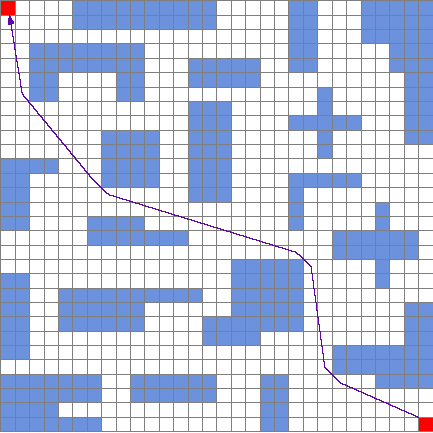
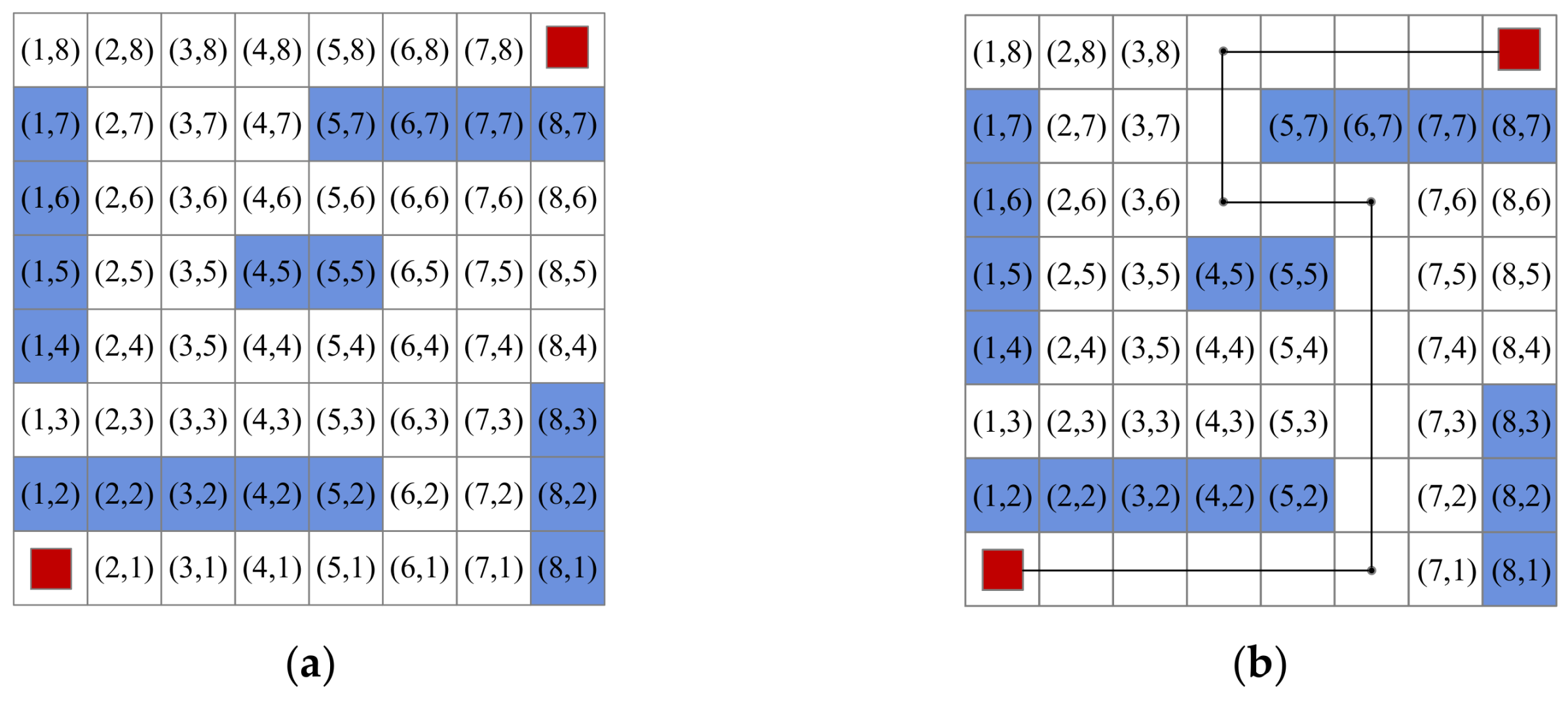
The selection of effective free cells in Section 4.1 is similar to the visibility graph concept in that collision-free points near the corners of obstacles are selected. In general, many studies that have utilized visibility graphs have set their free points near the corners of obstacles as nodes and checked whether each node is linked as shown in Figure 7.
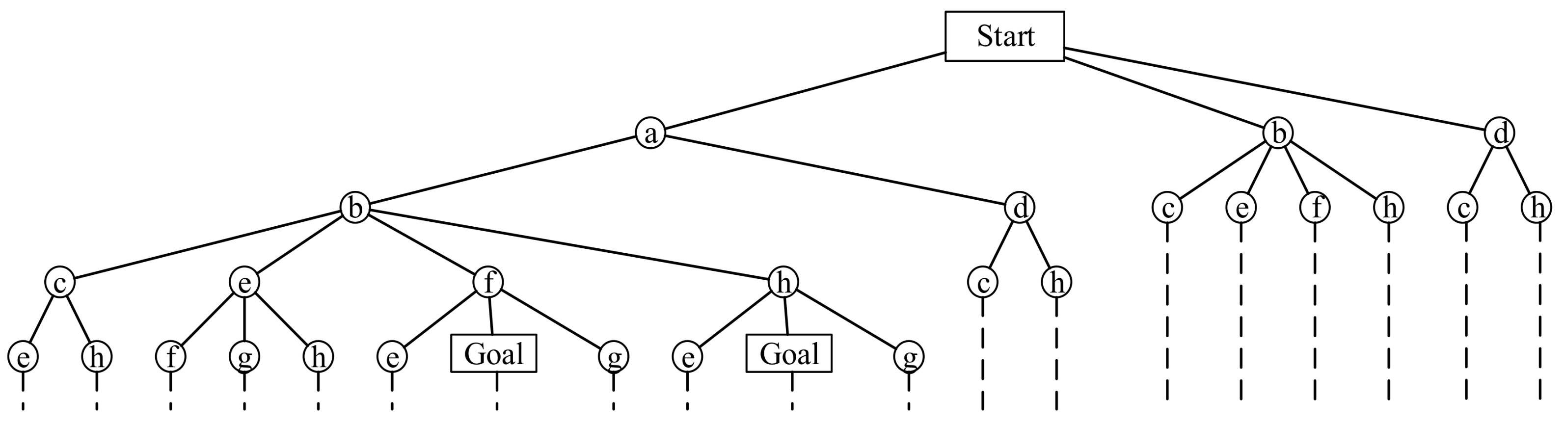
In other words, a path finding method using a visibility graph converts a map into a graph and uses tree search methods to find the shortest path as shown in Figure 8. In tree search methods, however, the time required to generate and calculate trees increases exponentially as the number of nodes increases.
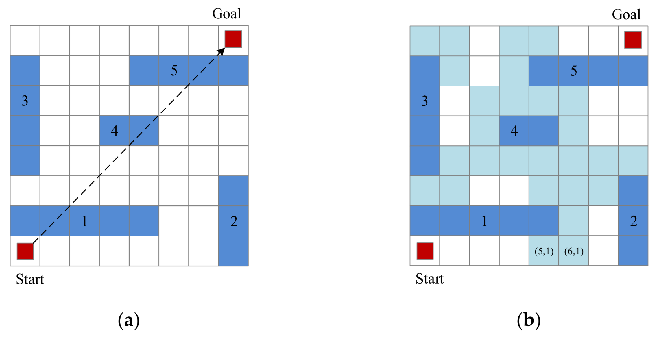
In this paper, the moving direction concept is considered for fast and effective path planning. There are numbers of obstacles in a given environment, but the critical obstacles that affect CFSPP are just part of the entire set of obstacles. One of the shortcomings of the visibility graph is that the directional information is missing when a map is converted into a graph. Directional information is important to determine critically affected obstacles. Figure 9 shows that the path finding is affected by only three of the five obstacles.
Since critically affected obstacles are a subset of the entire set of obstacles, the number of necessary selected free cells decreases compared to the visibility graph when the moving direction is considered. Therefore, this study deduces the moving direction of the MAs from the current cell to the goal cell, and it then narrows the range of selected effective free cells. If an MA is going to collide with an obstacle while it is moving in the given direction, it must detour around the obstacle to reach the goal cell. The selected effective free cells found in Section 4.1 are used to effectively detour around the obstacles.
4.3. Steps to Generate Feasible Paths
The following is a list of detailed algorithm steps.
- Step 0. Initialize the environment.
- Step 1. Check the current position to determine whether it is adjacent to any obstacles. If so, let the adjacent obstacle select any random effective free cell adjacent to obstacle i and update the current position to cell . If the current position is not adjacent to any obstacles, do not update the current position.
- Step 2. Deduce the moving direction from the current position to the goal position and move in that direction.
- Step 3. If an MA does not collide with any obstacles other than obstacle , connect the current position and goal position, and stop the algorithm. If an MA collides with an obstacle, set sub-start to current position and sub-goal to current destination. After this, continue to Step 4.
- Step 4. Let the obstacle the MA collides with first, be obstacle . Check whether any effective free cells adjacent to obstacle are linked to the current position. If so, continue to Step 5. If not, create a recursive function in which the goal point is set to a random effective free cell adjacent to obstacle considering direction factor, and go to Step 1.
- Step 5. The MA moves to a random effective free cell, , adjacent to obstacle and update the current position to cell .
- Step 6. Repeat Steps 1 to 5 until the MA reaches the goal point.
Figure 10, Figure 11, Figure 12 and Figure 13 are examples of generating initial chromosomes. In Figure 10a, the direction from the start point to the goal point is deduced, and an obstacle that an MA collides with when moving in the given direction is found. Figure 10a presents an example in which an MA collides with obstacle 1. In this case, the current position is the start point, and the effective free cells linked to the current position are (5, 1) and (6, 1), as shown in Figure 10b. The MA moves to a free cell randomly selected among these six cells. In this example, it is assumed that the MA moves to (6, 1).
Since cell (6, 1) is adjacent to obstacle 1, one effective free cell adjacent to obstacle 1 is randomly selected, as demonstrated in Step 1. Figure 11a shows that cell (5, 3) is selected. The direction from (5, 3) to the goal point is deduced. The MA collides with obstacle 5. The algorithm searches for effective free cells that link obstacle 5 to cell (5, 3), as demonstrated in Step 4, but no cells are found. Actually, there are no effective frees cells linking obstacles 1 and 5, as shown in Figure 11b.
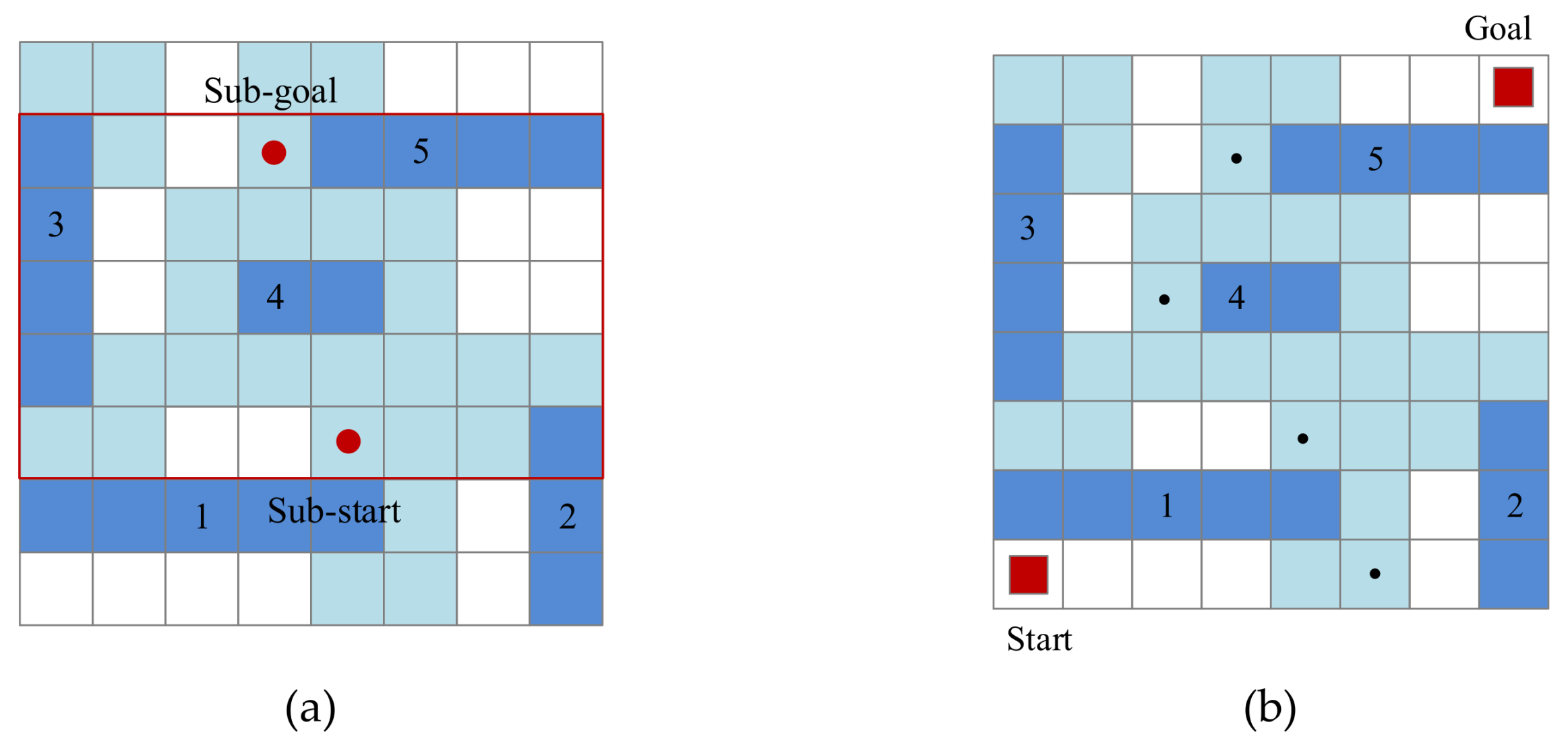
This means there is another obstacle between obstacles 1 and 5, and it prevents feasible paths from being generated. In this case, a feasible path from obstacle 1 to 5 can be found using a recursive function, as demonstrated in Step 4, splitting the original problem into a sub-problem. In Figure 12a, the sub-start point is set to one effective free cell next to obstacle 1, and the sub-goal is one of the effective free cells next to obstacle 5. Since obstacle 4 is blocking the path from obstacle 1 to 5, one effective free cell next to obstacle 4 is selected as a detour point. When choosing one of the effective free cells, a direction factor which includes distance from sub-start point to sub-goal point, and the direction derived by these two points is considered. If there are multiple direction factors that generate a comparable path, then it will choose the better path based on these direction factors, and this path forms detours or could be formed as another sub-problem. In this example, cell (3, 5) is selected, and the MA can reach the sub-goal. The sub-problem is solved, and the solution path is added to the path of the original problem.
The current position of the MA is cell (4, 7), and the free cell is adjacent to obstacle 5. When the MA moves from cell (4, 7) to the goal point following a linear line, it does not collide with any obstacles apart from obstacle 5. That is, some free cells next to obstacle 5 are directly linked to the goal point demonstrated in Step 3, and the algorithm stops as shown in Figure 12b.
Figure 13 shows the generated initial paths via the proposed algorithm. Paths from cell (6, 1) to (5, 3) and from (4, 7) to (8, 8) in Figure 13a generate infeasible paths, but two cells are adjacent to the same obstacle. It is assumed that all information is known. Therefore, a detour can be generated by moving along the edge of the obstacle. Following these procedures, Figure 13a becomes a feasible path, as shown in Figure 13b.
5. Genetic Algorithm
Applying the proposed methodology, a modified GA is introduced to solve CFSPP problems. Contrary to many previous studies that used random selection to generate feasible chromosomes, this study uses effective free cells and the moving direction of the MAs in its initializing, crossover, and mutation operations. Chromosomes are reproduced based on their ranking of fitness values, and a diversity of chromosomes is achieved with a random mutation operation. Details of the proposed modified GA follow below.
5.1. GA Model
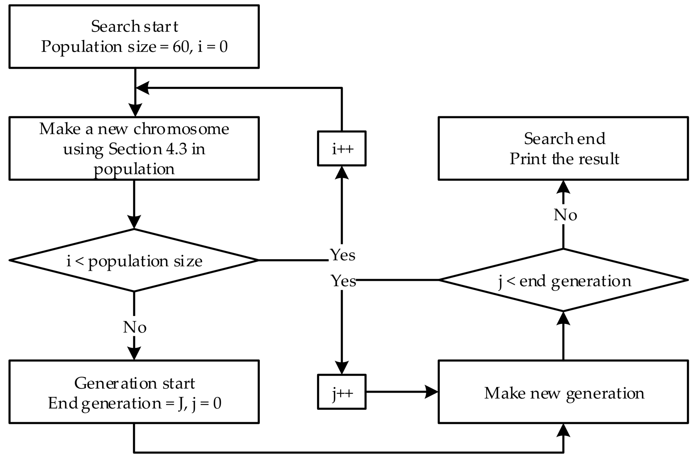
Figure 14 shows the flowchart of the GA model. At the beginning of the GA, a population is required to initialize the chromosomes. This paper uses 60 chromosomes in one population. Each generation produces a new population using the crossover and mutation operations. These processes are explained in Section 5.3 and Section 5.4.
5.2. Chromosome Reproduction
After evaluating the fitness values of each chromosome, the chromosomes are ranked in order of fitness values. Figure 15 shows the reproduction process. Top 20 chromosomes are carried down directly to the next generation, and the remaining 40 chromosomes are reproduced. Half of the bottom 40 chromosomes are reproduced via a crossover operation, and the other half is generated via a mutation operation.
5.3. Crossover
In the crossover operation, each parent chromosome is randomly selected from the top 20 chromosomes. A random gene, , in the parent chromosomes is selected as a swapping point, and offspring chromosomes are generated by swapping genes after the gene. Child 1 inherits the genes of Parent 1 before the gene, and then inherits genes from Parent 2. In the same manner, Child 2 inherits the genes of Parent 2 before the gene and then inherits genes from Parent 1. Figure 16, Figure 17 and Figure 18 demonstrate the crossover operation.
In the case depicted in Figure 16, Figure 16a, b show the parents of the crossover operation. These graphs are represented as chromosomes in Figure 17a. The crossover’s swapping point is set as the 5th gene of each chromosome.
Following the crossover, the children’s chromosomes are generated as Figure 17b. When the children are produced via the crossover operation, there is a chance that infeasible paths are created. For Child 1 in Figure 18a, cells (5, 3) and (4, 7) are neither linked, nor adjacent, to the same obstacle. When infeasible chromosomes are created, the two genes that make the path infeasible are set to the start and goal points, respectively, and they are modified into a feasible path with the algorithm proposed in Section 4.3. Child 2 in Figure 18c represents a solution that is infeasible due to a collision with an obstacle. Applying the same logic to this case, the results are shown in Figure 18d.
By using the proposed algorithm, a feasible path between cells (5, 3) and (4, 7) is generated, and Child 1 consists of (1, 1), (6, 1), (6, 2), (5, 3), (6, 5), (4, 7), (4, 8), and (8, 8).
5.4. Mutation
The mutation operation in the GA is important to retain the diversity of chromosomes and prevent trapping in the local minimum. This study adopts a random mutation. A chromosome among the top 20 is randomly selected. A random gene is selected from the selected chromosome. A mutant chromosome inherits the genes of the selected chromosome before the . gene, and it then generates a random path. Figure 19 shows the random mutation operation. In Figure 19, the chromosome brings the first three genes from the parent, and the rest of the chromosomes are filled via the process of finding feasible paths described in Section 4.3. This new chromosome represents a new solution that is the result of the mutation operation.
6. Experimental Results
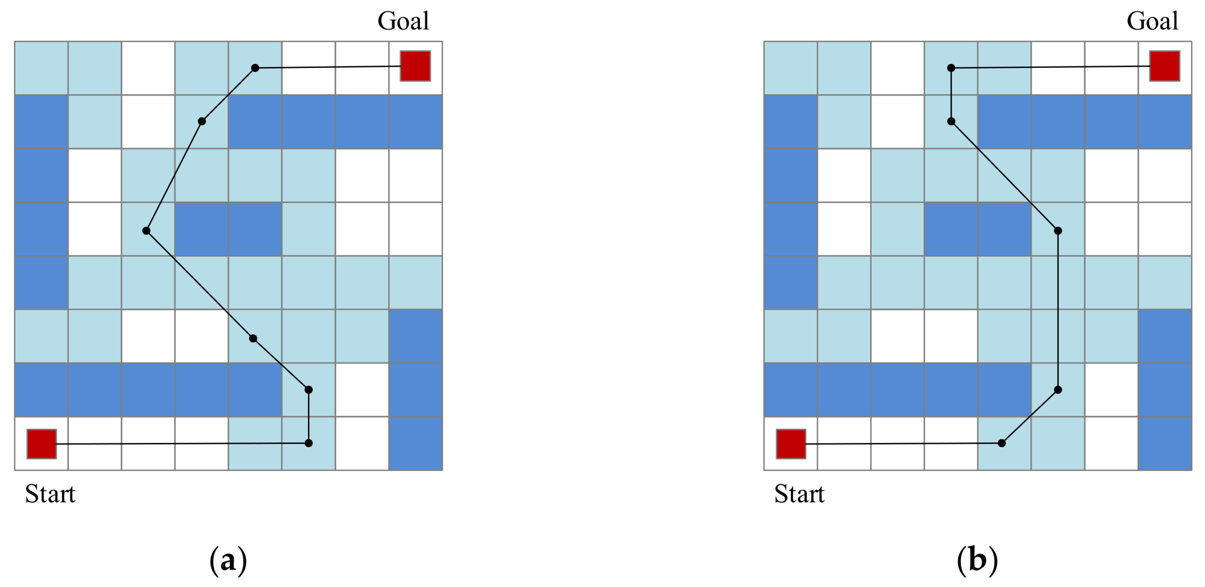
The proposed methodology and GA are implemented using the following specifications: Java jdk1.8, Intel Core i7-4790K central processing unit (CPU) (4.0 GHz) processor, 16 GB of memory, and Windows 10. Five different environments are experimented on to measure performances. Environments 1 and 2 are small cases with 16 x 16 grid spaces, and Environments 3 to 5 are bigger problems with 30 × 30 spaces. The GA is run 100 times for each environment. The experimental results for Environments 1 and 2 are compared to the results in previous studies. Environment 1 includes seven obstacles, and the MA moves from cell (1, 1) to (16, 16). In Environment 2, there are 10 obstacles, and the MA travels from cell (1, 16) to (16, 1). Figure 20 shows Environments 1 and 2.
In the two environments, the GA stops if the best fitness value does not update over 500 sequential generations. Table 1 and Table 2 show the results for Environments 1 and 2, respectively. The result of benchmark problem, Environment 1 and 2, are from the previous literature. [12,13,15] This study is designed to include the average of all fitness values, average running time of 100 trials, and best fitness value found in 100 trials.
In each environment, the best fitness value of the proposed method is better than [12,13], and the average of all fitness values is better than [13,15]. Average fitness value of this study is better than the best fitness value of [13,15]. Figure 21 shows the found collision-free shortest path in each environment.
It is also remarkable that the proposed method determines good paths much faster for both environments compared to the methods in previous research. Figure 22 shows that the proposed method converges very rapidly.
Table 3 shows that the deviation of fitness value is decreasing by time. The deviations of initial fitness values are remarkably high. As time goes on, the deviations are rapidly decreasing. The algorithm makes the fitness value converge towards a good solution consistently. This indicates that the algorithm tries diverse ways to find a solution at the initial stage, and it consistently converges to certain points which are assumed to be reasonably great at the end of iteration. This means that the algorithm follows the right track for diversification and intensification. We can expect that the algorithm generates very stable values at the termination stage for each instance.
Rapid convergences result from the narrowed search space scope. Table 4 shows the scopes of the search spaces in each environment. In both environments, the proposed method searches only limited free cells compared to the previous methodologies. Since the proposed methodology depends heavily on obstacles, when the number of obstacles increases, the search space scope also increases. Nevertheless, the proposed methodology always searches for smaller scopes than those searched for by the previous methodologies. This boosts rapid convergence and helps to determine good paths.
To ensure that the proposed methodology and GA perform well in more complex environments, this study introduces and conducts experiments with three complex 30 × 30 environments. Figure 23 shows Environments 3 to 5 and their collision-free shortest paths.
There are a large number of identical obstacles at regular intervals in Environment 3 and a relatively small number of large obstacles in Environment 4. Environment 5 is rather complex, as it includes many concave-shaped obstacles. In three environments, the GA stops if the best fitness value does not update over 2000 sequential generations.
Table 5 shows the average of all fitness values, the average running time of 100 trials, and the best fitness value found in 100 trials. Table 6 and Figure 24 shows the average of all fitness values over time.
The proposed method finds collision-free short paths very quickly in three environments. It took less than 1 second in Environment 4. Environments 3 and 5 took slightly longer than 1 second. Since the proposed method depends heavily on obstacles, when the number of obstacles increases, or when obstacle shapes become more complex, it requires a little more time, but is, nevertheless, reasonable. In more complex environments, the proposed method also determines good collision-free paths and converges very rapidly, regardless of environment size or obstacle shape.
Table 7 shows relationship between experimental space and CPU time. Environments 2 and 4 have a similar number of obstacles and effective free cells. However, the average CPU time of Environment 4 is about 5 times longer than Environment 2. Concurrently, Environments 3 and 4 have the same number of total cells, but the method found the solution much faster for Environment 4. This is because there are more obstacles and effective free cells in Environment 3 than Environment 4. The number of effective free cells are not directly proportional to the number of obstacles but there is higher chance of having more effective cells with more obstacles. Therefore, the required solution time depends on the number of cells and the number of effective free cells, which depends on the shape and number of obstacles.
7. Conclusions
In this paper, a novel methodology for a GA in CFSPP is introduced. Many previous studies have generated CFSPP by connecting randomly selected free points, but this free space-based random selection includes many infeasible paths, thereby causing slower convergence. On the other hand, the obstacle-based search methodology proposed in this study searches for short paths by finding critical obstacles first, and effectively detouring around them. Critical obstacles that affect CFSPP are mainly determined by considering the moving directions of the MAs, and effective free cells are selected based on the critical obstacles.
The proposed method can narrow the scope of the search spaces. This allows it to determine better collision-free shortest paths than random selection methods. Moreover, the proposed method simplifies the given problems by splitting them into small sub-problems, in some specific cases. As such, the method can reduce problem complexity.
An additional experiment has been conducted to show the methodology’s applicability to more complex problems (i.e., Environments 3 to 5). The proposed direction-based GA generates favorable solutions very quickly—within a maximum of 2 s—despite the increased problem size. This suggests that the proposed method could be applied to real world problems that are very large and contain complex obstacles, such as irregular shapes.
Although this paper only employs static environments, the short convergence time shows that the proposed method and algorithm could be applied to dynamic environments in which real-time path planning is necessary. The proposed ideas could also be applied to 3-dimensional environments for UAVs, with more constraints for practical cases in future research.
This research focused on searching for efficient and effective paths for MAs in static environments. However, the current state of art in MAs indicates that the limited resources of MA to compute the best path is expanding to generate the path in dynamic environments in a reasonable time. This could direct our future research. We could apply the evolutionary algorithm to search for the path when the MA is assigned to move from origin to destination without a predefined path. Additionally, we assumed the solution space is in a 2D environment, but we could expand the dimensions of possible paths for MA, which is possible to apply to UAVs.
Author Contributions
Conceptualization, J.C and H.-Y.L. Methodology, H.-Y.L.; Validation, H.-Y.L. and H.S. Formal Analysis, H.-Y.L and H.S.; Writing—Original Draft Preparation, H.-Y.L.; Supervision, J.C.; Writing—Review & Editing, H.S. and J.C.; Implementing the algorithm and the experiment were mostly carried out by H.-Y.L. and H.S. under the supervision of J.C.
Funding
This work was supported by a 2017 Korea Aerospace University faculty research grant.
Conflicts of Interest
The authors declare no conflict of interest.
Appendix A. Dynamic Environment
When MAs detect a change of obstacles during the path planning process, the path should be changed as a reflection of obstacle changes, which is referred to as a dynamic environment [13,15]. The dynamic simulation environment, as shown in Figure A1a,b, is applied to compare the results with [13,15]. In Figure A1b, a new obstacle appears, and the original solution in Figure A1a is no longer feasible, and the algorithm needs to start the process to find the best path. The algorithm finds the solution in a relatively short time, and it swiftly responds to the change in environment. Li et al. [13] made a scenario in which an obstacle is added, as shown in Figure A1a,b.
Figure A1.
Dynamic environment scenario. (a) Origin Environment 1; (b) changed Environment 1.


Table A1.
The result of dynamic environment scenario.
| Environment Name | Item | Li et al. [13] | Tuncer and Yildirim [15] | This Study |
|---|---|---|---|---|
| Original E1 | fitness value (average) | 29.25 | 27.82 | 27.22 |
| CPU time (s) (average) | 0.31 | 0.89 | 0.16 | |
| best fitness value | 27.22 | - | 27.22 | |
| Changed E1 | fitness value (average) | 31.21 | 29.08 | 28.67 |
| CPU time (s) (average) | 0.26 | 0.86 | 0.10 | |
| best fitness value | 28.73 | - | 28.65 |
The results of [13,15], and this study, under dynamic environment scenario, are shown in Table A1. This study finds better average fitness values than that of Li et al. [13] and Tuncer and Yildirim [15]. In the Original Environment 1, the average fitness value in this study is the same as the best fitness value. This means that the proposed algorithm consistently found the best solution for the problem. In terms of CPU time, the algorithm finds the solution in a relatively short time, even though the time measure is not directly comparable. We can expect that the path would be shorter, again, if the obstacle, which appears after the original environment, disappears.
References
- Banker, S. Robots In The Warehouse: It’s Not Just Amazon. Forbes. 2016. Available online: https://www.forbes.com/sites/stevebanker/2016/01/11/robots-in-the-warehouse-its-not-just-amazon/#49c4019840b8 (accessed on 20 July 2017).
- Amazon makes first drone delivery. BBC. 2016. Available online: https://www.bbc.com/news/technology-38320067 (accessed on 15 August 2017).
- Siegwart, R.; Nourbakhsh, I.R.; Scaramuzza, D. Introduction to Autonomous Mobile Robots; MIT Press: Cambridge, MA, USA, 2011. [Google Scholar]
- Van Den Berg, J.; Ferguson, D.; Kuffner, J. Anytime path planning and replanning in dynamic environments. In Proceedings of the IEEE International Conference on Robotics and Automation, Orlando, FL, USA, 15–19 May 2006; pp. 2366–2371. [Google Scholar] [CrossRef]
- Mac, T.T.; Copot, C.; Tran, D.T.; De Keyser, R. Heuristic approaches in robot path planning: A survey. Robot. Auton. Syst. 2016, 86, 13–28. [Google Scholar] [CrossRef]
- Gao, M.; Xu, J.; Tian, J.; Wu, H. Path Planning for Mobile Robot Based on Chaos Genetic Algorithm. In Proceedings of the 2008 Fourth International Conference on Natural Computation, Jinan, China, 18–20 October 2008; pp. 409–413. [Google Scholar] [CrossRef]
- Gemeinder, M.; Gerke, M. GA-based path planning for mobile robot systems employing an active search algorithm. Appl. Soft Comput. 2003, 3, 149–158. [Google Scholar] [CrossRef]
- Sugihara, K.; Smith, J. Genetic Algorithms for Adaptive Motion Planning of an Autonomous Mobile Robot. In Proceedings of the 1997 IEEE International Symposium on Computational Intelligence in Robotics and Automation, Monterey, CA, USA, 10–11 July 1997; pp. 138–143. [Google Scholar] [CrossRef]
- Daniel, K.; Nash, A.; Koenig, S.; Felner, A. Theta *: Any-Angle Path Planning on Grids. J. Artif. Intell. Res. 2010, 39, 533–579. [Google Scholar] [CrossRef]
- Hu, Y.; Yang, S.X. A knowledge based genetic algorithm for path planning of a mobile robot. In Proceedings of the IEEE International Conference on Robotics and Automation (ICRA’04), New Orleans, LA, USA, 26 April–1 May 2004; Volume 5, pp. 4350–4355. [Google Scholar] [CrossRef]
- Huang, H.; Tsai, C. Global path planning for autonomous robot navigation using hybrid metaheuristic GA-PSO algorithm. In Proceedings of the SICE Annual Conference (SICE), Tokyo, Japan, 13–18 September 2011; pp. 1338–1343. [Google Scholar]
- Karami, A.H.; Hasanzadeh, M. An adaptive genetic algorithm for robot motion planning in 2D complex environments. Comput. Electr. Eng. 2015, 43, 317–329. [Google Scholar] [CrossRef]
- Li, Q.; Zhang, W.; Yin, Y.; Wang, Z.; Liu, G. An Improved Genetic Algorithm of Optimum Path Planning for Mobile Robots. In Proceedings of the Sixth International Conference on Intelligent Systems Design and Applications, Jinan, China, 16–18 October 2006; Volume 2, pp. 637–642. [Google Scholar] [CrossRef]
- Sedighi, K.H.; Ashenayi, K.; Manikas, T.W.; Wainwright, R.L.; Tai, H. Autonomous Local Path Planning for a Mobile Robot Using a Genetic Algorithm. Electr. Eng. 2004, 1338–1345. [Google Scholar] [CrossRef]
- Tuncer, A.; Yildirim, M. Dynamic path planning of mobile robots with improved genetic algorithm. Comput. Electr. Eng. 2012, 38, 1564–1572. [Google Scholar] [CrossRef]
- Frontzek, T.; Goerke, N.; Eckmiller, R. Flexible Path Peal-Time Applications Using A*-Method and Neural RBF-Networks. In Proceedings of the 1998 IEEE International Conference on Robotics and Automation, Leuven, Belgium, 16–20 May 1998; pp. 1417–1422. [Google Scholar]
- Juidette, H.; Youlal, H. Fuzzy dynamic path planning using genetic algorithm. Electron. Lett. 2000, 36, 374–376. [Google Scholar]
- Miao, H.; Tian, Y.-C. Dynamic robot path planning using an enhanced simulated annealing approach. Appl. Math. Comput. 2013, 222, 420–437. [Google Scholar] [CrossRef] [Green Version]
- Khatib, O. Real-time obstacle avoidance for manipulators and mobile robots. Int. J. Robot. Res. 1986, 5, 396–404. [Google Scholar] [CrossRef]
- Wang, C.; Soh, Y.C.; Wang, H.; Wang, H. A hierarchical genetic algorithm for path planning in a static environment with obstacles. In Proceedings of the Canadian Conference on Electrical and Computer Engineering (IEEE CCECE 2002), Winnipeg, MB, Canada, 12–15 May 2002; pp. 1652–1657. [Google Scholar]
- Lozano-Pérez, T.; Wesley, M.A. An algorithm for planning collision-free paths among polyhedral obstacles. Commun. ACM 1979, 22, 560–570. [Google Scholar] [CrossRef]
- Rashid, A.T.; Ali, A.A.; Frasca, M.; Fortuna, L. Path planning with obstacle avoidance based on visibility binary tree algorithm. Robot. Auton. Syst. 2013, 61, 1440–1449. [Google Scholar] [CrossRef]
- Janson, L.; Ichter, B.; Pavone, M. Deterministic sampling-based motion planning: Optimality, complexity, and performance. Int. J. Robot. Res. 2018, 37, 46–61. [Google Scholar] [CrossRef]
- Lin, Y.; Saripalli, S. Sampling-Based Path Planning for UAV Collision Avoidance. IEEE Trans. Intell. Transp. Syst. 2017, 18, 3179–3192. [Google Scholar] [CrossRef]
- Wei, K.; Ren, B. A Method on Dynamic Path Planning for Robotic Manipulator Autonomous Obstacle Avoidance Based on an Improved RRT Algorithm. Sensors 2018, 18, 571. [Google Scholar] [CrossRef] [PubMed]
- Aguilar, W.G.; Morales, S.G. 3D Environment Mapping Using the Kinect V2 and Path Planning Based on RRT Algorithms. Electronics 2016, 5, 70. [Google Scholar] [CrossRef]
- Mohanty, P.K.; Parhi, D.R. Optimal path planning for a mobile robot using cuckoo search algorithm. J. Exp. Theor. Artif. Intell. 2016, 28, 35–52. [Google Scholar] [CrossRef]
- Englot, B.; Hover, F. Multi-goal feasible path planning using ant colony optimization. In Proceedings of the 2011 IEEE International Conference on Robotics and Automation, Shanghai, China, 9–13 May 2011; pp. 2255–2260. [Google Scholar] [CrossRef]
- Wang, X.; Xue, L.; Yan, Y.; Gu, X. Welding Robot Collision-Free Path Optimization. Appl. Sci. 2017, 7, 89. [Google Scholar] [CrossRef]
- Raja, P. Optimal path planning of mobile robots: A review. Int. J. Phys. Sci. 2012, 7, 1314–1320. [Google Scholar] [CrossRef]
- Karaman, S.; Frazzoli, E. Sampling-based algorithms for optimal motion planning. Int. J. Robot. Res. 2011, 30, 846–894. [Google Scholar] [CrossRef] [Green Version]
- Roberge, V.; Tarbouchi, M.; Labonte, G. Comparison of parallel genetic algorithm and particle swarm optimization for real-time UAV path planning. IEEE Trans. Ind. Inform. 2013, 9, 132–141. [Google Scholar] [CrossRef]
- Bottasso, C.L.; Leonello, D.; Savini, B. Path planning for autonomous vehicles by trajectory smoothing using motion primitives. IEEE Trans. Control Syst. Technol. 2008, 16, 1152–1168. [Google Scholar] [CrossRef]
- Scheuer, A.; Fraichard, T. Continuous-curvature path planning for car-like vehicles. In Proceedings of the 1997 IEEE/RSJ International Conference on Intelligent Robot and Systems. Innovative Robotics for Real-World Applications (IROS ’97), Grenoble, France, 11 September 1997; Volume 2, pp. 997–1003. [Google Scholar] [CrossRef]
- Tsai, C.-C.; Huang, H.-C.; Chan, C.-K. Parallel Elite Genetic Algorithm and Its Application to Global Path Planning for Autonomous Robot Navigation. IEEE Trans. Ind. Electron. 2011, 58, 4813–4821. [Google Scholar] [CrossRef]
- De Boor, C. On calculating with B-splines. J. Approx. Theory 1972, 6, 50–62. [Google Scholar] [CrossRef]
- Cox, M.G. The numerical evaluation of B-splines. IMA J. Appl. Math. 1972, 10, 134–149. [Google Scholar] [CrossRef]
- Jia, D.; Vagners, J. Parallel evolutionary algorithms for UAV path planning. In Proceedings of the AIAA 1st Intelligent Systems Technical Conference, Chicago, IL, USA, 20–22 September 2004. [Google Scholar] [CrossRef]
Figure 1.
Restricted moving directions.

Figure 2.
Shortest path with different direction limitations (a) under direction limitation; (b) without direction limitation.
Figure 2.
Shortest path with different direction limitations (a) under direction limitation; (b) without direction limitation.

Figure 3.
Environment representation. (a) XY positions; (b) an example of detour.

Figure 4.
Detour efficiency. (a) Inefficient detour; (b) efficient detour.

Figure 5.
Selecting effective free cells. (a) Efficient free cells of one obstacle; (b) total efficient free cell.
Figure 5.
Selecting effective free cells. (a) Efficient free cells of one obstacle; (b) total efficient free cell.

Figure 6.
Connecting free cells to enable a path. (a) Unlinked cells; (b) linked cells.

Figure 7.
Narrowing the searching space to network.

Figure 8.
Visibility tree search.

Figure 9.
Obstacles in collision-free shortest path planning (CFSPP).

Figure 10.
Selecting an effective free cell. (a) Direct path from the start to the goal; (b) effective free cells.
Figure 10.
Selecting an effective free cell. (a) Direct path from the start to the goal; (b) effective free cells.

Figure 11.
Selecting free cells to avoid obstacles. (a) A path from the selected free cell to the goal; (b) searching paths for the first free cell.
Figure 11.
Selecting free cells to avoid obstacles. (a) A path from the selected free cell to the goal; (b) searching paths for the first free cell.

Figure 12.
Generating sub-problems. (a) Defined sub-problem; (b) selected free cells for a feasible path.
Figure 12.
Generating sub-problems. (a) Defined sub-problem; (b) selected free cells for a feasible path.

Figure 13.
Modifying two infeasible cells for the same obstacle. (a) An infeasible solution; (b) detour path generated to maintain feasibility.
Figure 13.
Modifying two infeasible cells for the same obstacle. (a) An infeasible solution; (b) detour path generated to maintain feasibility.

Figure 14.
Flow of search process.

Figure 15.
Reproduction of chromosomes.

Figure 16.
Parents of the crossover operation (a) Parent 1; (b) Parent 2.

Figure 17.
Chromosomes of crossover operation (a) two parents’ chromosomes; (b) generated chromosomes via crossover operation.
Figure 17.
Chromosomes of crossover operation (a) two parents’ chromosomes; (b) generated chromosomes via crossover operation.

Figure 18.
Children of crossover operation. (a) Original Child 1; (b) modified Child 1; (c) original Child 2; (d) modified Child 2.
Figure 18.
Children of crossover operation. (a) Original Child 1; (b) modified Child 1; (c) original Child 2; (d) modified Child 2.

Figure 19.
Path mutation. (a) Chromosome; (b) mutation operation on graph.

Figure 20.
Representation of environments. (a) Environment 1; (b) Environment 2.

Figure 21.
Collision-free shortest paths in environments. (a) Environment 1; (b) Environment 2.

Figure 22.
Rapid convergence of proposed method in environments. (a) Environment 1; (b) Environment 2.
Figure 22.
Rapid convergence of proposed method in environments. (a) Environment 1; (b) Environment 2.

Figure 23.
Grid-based representation and collision-free shortest paths in environments. (a) Environment 3; (b) Environment 4; (c) Environment 5.
Figure 23.
Grid-based representation and collision-free shortest paths in environments. (a) Environment 3; (b) Environment 4; (c) Environment 5.

Figure 24.
Plot of average distances over time.

Table 1.
Comparison of results in Environment 1.
| Study | Fitness Value (Average) | CPU Time (s) (Average) | Best Fitness Value |
|---|---|---|---|
| Li et al. [13] | 31.21 | 0.26 | 28.73 |
| Tuncer and Yildirim [15] | 29.08 | 0.86 | - |
| Karami and Hasanzadeh [12] | - | 3.47 | 28.87 |
| This study | 28.67 | 0.10 | 28.65 |
Table 2.
Comparison of results in Environment 2.
| Study | Fitness Value (Average) | CPU Time (s) (Average) | Best Fitness Value |
|---|---|---|---|
| Li et al. [13] | 25.17 | 0.34 | - |
| Tuncer and Yildirim [15] | 24.71 | 0.69 | - |
| Karami and Hasanzadeh [12] | - | 3.62 | 23.59 |
| This study | 23.46 | 0.13 | 22.84 |
Table 3.
Average fitness value and deviation of fitness value in Environment 1 (E1) and 2 (E2).
| Time (s) | E1 | E2 | ||
|---|---|---|---|---|
| Average | Deviation | Average | Deviation | |
| initial fitness | 42.27114 30.32668 | 1.587456 1.040444 | 44.01728 26.92745 | 4.493747 1.952633 |
| 0.01 | ||||
| 0.05 | 28.75185 | 0.016225 | 24.85468 | 0.355333 |
| 0.1 | 28.72511 | 0.007467 | 24.06891 | 0.265282 |
| 0.2 | 28.69232 | 0.004177 | 23.98146 | 0.211417 |
| 0.5 | 28.67255 | 0.001941 | 23.51231 | 0.153957 |
Table 4.
Comparison of selectable free cells in Environments 1 and 2.
| Attribute | E1 | E2 |
|---|---|---|
| # of total cells | 256 | |
| # of obstacles | 7 | 10 |
| # of blocked cells | 65 | 98 |
| # of free cells | 189 | 156 |
| # of selectable cells in random selection | 189 | 156 |
| # of selectable cells in this study | 24 | 55 |
Table 5.
Obtained results in Environments 3, 4, and 5.
| Environment # | Fitness Value (Average) | CPU Time (s) (Average) | Best Fitness Value |
|---|---|---|---|
| E3 | 43.84 | 1.17 | 42.95 |
| E4 | 52.06 | 0.67 | 50.49 |
| E5 | 46.82 | 1.87 | 45.52 |
Table 6.
Average distances over time in Environments 3, 4, and 5.
| Times (s) | E3 | E4 | E5 |
|---|---|---|---|
| initial fitness | 83.26 | 134.6274 | 210.25 |
| 0.01 | 56.38 | 66.30 | 91.67 |
| 0.05 | 45.09 | 56.44 | 50.35 |
| 0.1 | 44.64 | 54.64 | 48.96 |
| 0.2 | 44.36 | 53.22 | 48.02 |
| 0.5 | 44.12 | 52.14 | 47.69 |
| 1 | 43.79 | 51.85 | 47.10 |
| 2 | 43.67 | 51.77 | 46.68 |
| 3 | 43.53 | 51.83 | 46.53 |
Table 7.
Comparison of experimental spaces and results between each Environment.
| Environment # | E1 | E2 | E3 | E4 | E5 |
|---|---|---|---|---|---|
| # of total cells | 256 | 256 | 900 | 900 | 900 |
| # of obstacles | 7 | 10 | 27 | 11 | 19 |
| # of effective free cells | 62 | 79 | 270 | 87 | 219 |
| Average CPU time (s) | 0.10 | 0.13 | 1.17 | 0.67 | 1.87 |
| Average fitness value | 28.67 | 23.46 | 43.84 | 52.06 | 46.82 |
© 2018 by the authors. Licensee MDPI, Basel, Switzerland. This article is an open access article distributed under the terms and conditions of the Creative Commons Attribution (CC BY) license (http://creativecommons.org/licenses/by/4.0/).
Share and Cite
MDPI and ACS Style
Lee, H.-Y.; Shin, H.; Chae, J. Path Planning for Mobile Agents Using a Genetic Algorithm with a Direction Guided Factor. Electronics 2018, 7, 212. https://doi.org/10.3390/electronics7100212
AMA Style
Lee H-Y, Shin H, Chae J. Path Planning for Mobile Agents Using a Genetic Algorithm with a Direction Guided Factor. Electronics. 2018; 7(10):212. https://doi.org/10.3390/electronics7100212
Chicago/Turabian StyleLee, Hyeok-Yeon, Hyunwoo Shin, and Junjae Chae. 2018. "Path Planning for Mobile Agents Using a Genetic Algorithm with a Direction Guided Factor" Electronics 7, no. 10: 212. https://doi.org/10.3390/electronics7100212
Note that from the first issue of 2016, this journal uses article numbers instead of page numbers. See further details here.