Abstract
In this paper, we propose a hardware-based architecture for automatic blue whale calls classification based on short-time Fourier transform and multilayer perceptron neural network. The proposed architecture is implemented on field programmable gate array (FPGA) using Xilinx System Generator (XSG) and the Nexys-4 Artix-7 FPGA board. This high-level programming tool allows us to design, simulate and execute the compiled design in Matlab/Simulink environment quickly and easily. Intermediate signals obtained at various steps of the proposed system are presented for typical blue whale calls. Classification performances based on the fixed-point XSG/FPGA implementation are compared to those obtained by the floating-point Matlab simulation, using a representative database of the blue whale calls.
1. Introduction
In the last decades, many pattern recognition systems have been proposed in various signal processing fields such as speech recognition, speaker identification/verification, musical instrument identification, biomedical signal classification, bioacoustic signal recognition, etc. A typical pattern recognition system is composed of two main blocks: feature extraction and classification. The feature extraction is the process that transform the pattern signal from original high-dimensional representation into lower–dimensional space, while the classification task operates to associate the signal pattern to one of predefined classes. The literature review shows that discrete Fourier transform (DFT), mel frequency cepstral coefficients (MFCC), linear predictive coefficients (LPC), discrete wavelet transform (DWT), and time–frequency contours have been used for feature extraction, while artificial neural networks (ANN), support vector machine (SVM), Gaussian mixture models (GMM), vector quantization (VQ), Fisher’s discriminant analysis (FD), and k–nearest neighbor (k–NN), classification and regression tree (CART), dynamic time warping (DTW), and hidden Markov models (HMM) have been used for the recognition/classification task.
Analysis of underwater bioacoustic signal has been the object of numerous publications, where several approaches have been proposed to recognize and classify these signals [1,2,3,4,5,6,7,8,9,10,11,12,13,14]. Much like birds, marine mammals are highly vocalizing animals and different species can be recognized by their specific sounds [15]. Among them, the blue whales produce regular and powerful low-frequency (<100 Hz) vocalizations that can propagate over distances exceeding 100 km [16]. The North Atlantic blue whales produce three specific vocalizations (Figure 1): the stereotyped A and B infrasonic calls (15–20 Hz) and more variable audible D or arch call (35–120 Hz). From blind recordings at a given location, these calls can be used to identify the species. Recordings using hydrophone array allow to localizing the callers [17].
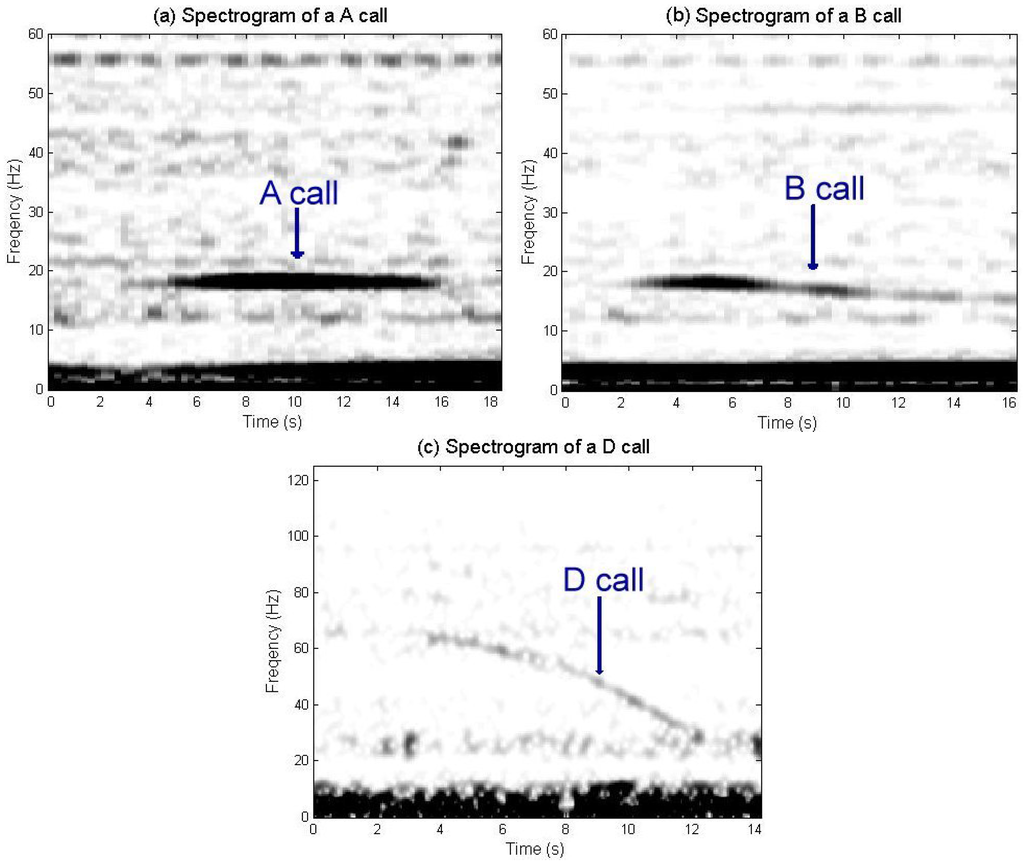
Figure 1.
Spectrogram of an A call (a), a B call (b), and a D call (c).
The pattern recognition algorithms were generally developed and optimized using software platform such as Matlab (R2012b, MathWorks, Natick, MA, USA, 2012). However, many applications require hardware implementation of these algorithms into real-time embedded systems. Hardware implementation remains a great challenge that requires tradeoff between accuracy, resource, and computation speed [18,19]. Most of the hardware-based architectures are proposed for speech and speaker recognition using digital signal processor (DSP) [20] or field programmable gate array (FPGA) [21,22,23,24,25,26]. FPGAs are generally preferred to the other hardware approaches because they combine the high-performance of the application-specific integrated circuits (ASICs) and the flexibility of the DSPs.
However, to the best of our knowledge, no hardware architecture has been proposed in the literature to classify/recognize bioacoustic signals. In this paper, we propose a hardware implementation of an automatic blue whale calls recognition based on the short-time Fourier transform (STFT) and the multilayer perceptron (MLP) neural network. Based on our previous algorithm developed using Matlab software [10], the proposed architecture has been optimized and implemented on FPGA using Xilinx System Generator (XSG) and Nexys-4 Artix-7 FPGA board. This architecture takes advantage of the native parallelism of the FPGA chips, instead of sequential processors implemented on these chips [27]. The main contributions are: (1) Optimization of the MLP-based classifier by reducing the number of its hidden neurons; (2) Development of XSG-based models of the mathematical equations describing the characterisation/classification algorithm to be implemented on FPGA; (3) Optimization of the required resources by reducing the fixed-point data format.
2. Method
Figure 2 represents the block diagram of a typical classification system, which is composed of the two main blocks: feature extraction and classification.
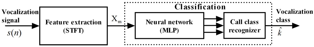
Figure 2.
Block diagram of a typical classification system based on short-time Fourier transform (STFT) and multilayer perceptron (MLP) neural network.
2.1. Feature Extraction
The implemented technique is based on the short-time Fourier transform (STFT) to extract a reduced number of features from two frequency subbands corresponding to the AB phrase and vocalization D, respectively [10,11]. The vocalization signal is split into successive frames before applying the STFT to each frame in order to extract 12-dimensional feature vector (Figure 3).
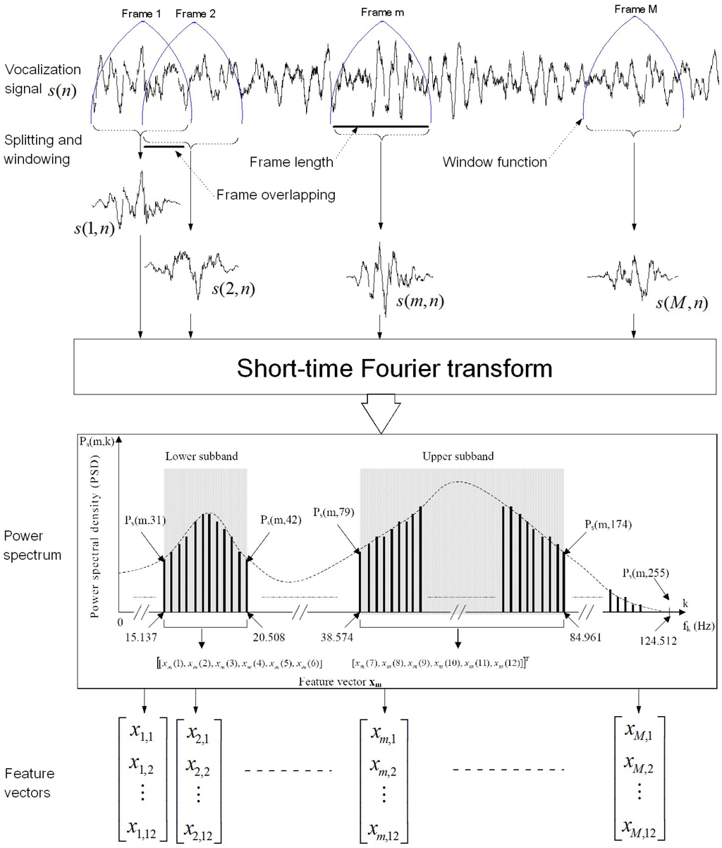
Figure 3.
Feature extraction process based on the short-time Fourier transform (STFT). Power spectrum density of each signal frame is computed using the STFT. The feature vector is constructed by extracting six components from lower subband (15.1375–20.508 Hz) and six components from upper subband (38.574–84.961 Hz). The discrete frequencies are obtained with a sampling frequency of 250 Hz and a frame length of 512 samples.
2.1.1. Signal Windowing
The vocalization signal is divided into consecutive frames of N samples, , where m is the frame index and n is the time index within the analyzed frame.
where is a window function of N samples. This function is located at , where L is the shift time step in samples. Hamming window is usually selected to reduce signal discontinuities during the segmentation and their resulting spectral artifacts.
2.1.2. Short-Time Fourier Transform
The short-time Fourier transform (STFT) of a given frame is defined by:
where N is the number of discrete frequencies that is usually chosen to be a power-of-2 in order to use the fast Fourier transform (FFT) algorithm, , and k is the frequency index ().
2.1.3. Power Spectrum
The power spectrum density (PSD) is computed from the complex Fourier spectrum using
At the sampling frequency , each signal frame is represented by N-points PSD covering the frequency range . As the power spectrum is symmetric, it can be described by only discrete frequencies. Each frequency index k represents a discrete frequencies , where .
2.1.4. Feature Vector Calculation
This method extracts features from two subbands (15.137–20.508 Hz) and (38.574–84.961 Hz) corresponding to the AB and D calls frequency ranges, respectively [10,11] (Figure 3). The first six components of the feature vector are calculated by averaging PSD points between and by bins of 2 points. The last six features are similarly calculated for the PSD interval from to but with bins of 16 points. The feature vector components, of a given frame m, are defined by
Thus, the analyzed frame, , will be characterized by the extracted feature vector, , where T represents the transpose operation.
2.2. Classification
Based on the extracted features vectors from a given vocalization, the classification task operates to associate this vocalization to one of predefined classes. The multi-layer Perceptron (MLP) is probably the most popular and the simplest artificial neural network that can be used for this kind of classification problems [10,11]. However, other techniques such as vector quantization (VQ), k–nearest neighbour (k–NN) and Gaussian mixture models (GMM) can also be employed.
2.2.1. Multilayer Perceptron
The MLP neural network is a set of several interconnected neurons arranged in layers: an input layer that acts as a data buffer, one or more hidden layers, and an output layer. Figure 4 represents an example of a MLP network characterized by = 12 inputs, one hidden layer of neurons, and = 3 outputs. Each hidden neuron j receives the output of each node i from the input layer through a connection of weight and then produce a corresponding response which is forwarded to the output layer. In fact, each neuron j performs a weighted sum that is transferred by a nonlinear function according to
where represents the bias of the jth hidden neuron. Similarly, the output of neuron k, in output layer, is defined by:
where is the activation function, is synaptic weight relating the output of the neuron in the hidden layer to the neuron of the output layer, and is the bias of the output neuron. The activation functions of the hidden neurons are typically hyperbolic tangent or logistic sigmoid. However, those of the output neurons can be linear or non-linear depending on the task performed by the network: a function approximation or a classification, respectively. In the proposed architecture, we used a logistic sigmoid function for neurons of both layers.
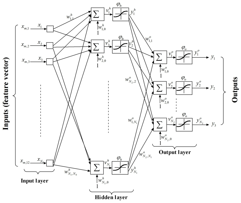
Figure 4.
Example of multi-layer perception (MLP) network network having = 12 inputs, one hidden layer of neurons, and = 3 outputs.
The connection weights and biases are determined in the training phase using a set of inputs for which the desired outputs are known . In the pattern recognition problems, the desired or target outputs are vectors of components, where = 3 is the number of the reference classes. For each desired vector , only one component, corresponding to the presented input pattern , is set to 1 and the others are set to 0. To accomplish the training task, the backpropagation (BP) algorithm is commonly used [28]. For the implemented architecture, the training phase is performed on Matlab and the resulting weights and biases are transferred to the XSG constant blocks.
2.2.2. Class Recognition
To classify an unknown vocalization, the observation sequence , corresponding to the feature vectors obtained from M adjacent segments of this vocalization, is presented to the MLP neural network that responds by the actual output sequence . For each output k, the network provides a set of M values . To classify the entire vocalization, the means of the values obtained over frames at the neural network outputs are commonly used. The unknown vocalization is associated to the reference call that corresponds to the largest mean value of the individual outputs:
where the mean values are computed over the M frames.
3. FPGA Implementation
Our objective is to propose a hardware-based architecture for automatic blue whale calls classification. The FPGAs have been chosen over the other hardware approaches because they combine the high-performance of the ASICs and the flexibility of DSPs. FPGAs are programmed using Hardware Description Languages (HDL) such as VHDL and Verilog, which require much experience with the hardware design and remain time consuming to perform the low-level description and debugging of the circuit to be mapped on FPGAs. In our case, we opted for a high-level programming tool (XSG) that allows us, with a high-level of abstraction, to design, simulate and execute the compiled design in the Matlab/Simulink environment quickly and easily. Once the XSG-based architecture is verified in Simulink, it can automatically be mapped to hardware implementation by Xilinx ISE Design Suite. The above techniques for feature extraction and classification were implemented on FPGA using the architecture presented in Figure 5, Figure 6, Figure 7 and Figure 8, where the main parts are described in the following subsections.
3.1. Signal Windowing
The windowed signal was obtained by multiplying the input signal with a Hamming window of samples, stored in a read only memory (ROM). The Xilinx ROM block is driven by a modulo–N cyclic counter [29] (Figure 5).
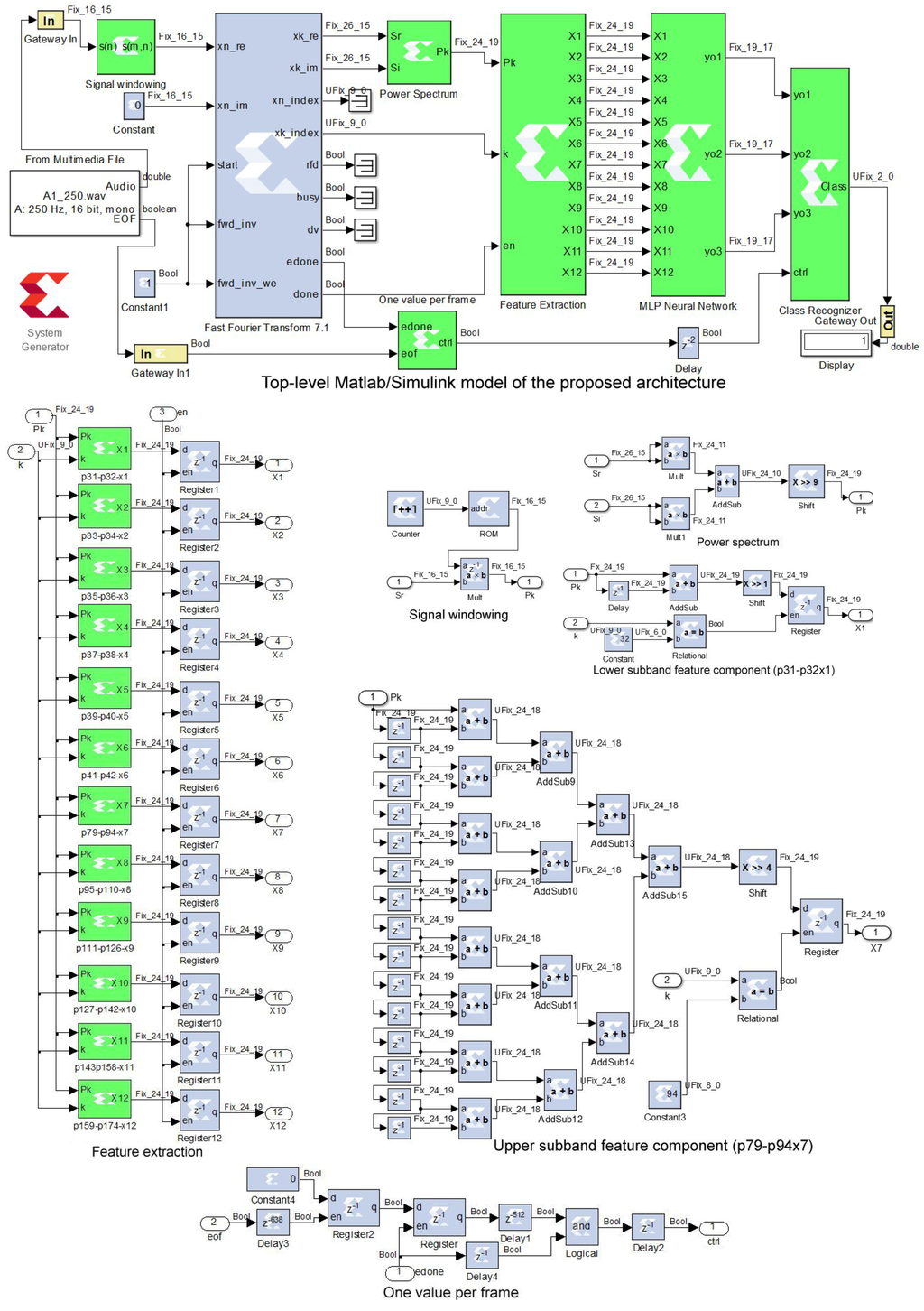
Figure 5.
Implementation of the proposed classification technique on field programmable gate array (FPGA) using Xilinx System Generator (XSG). The top-level Simulink diagram (top panel) with details of different subsystems (bottom panels). The green blocks are designed using the XSG blocks (blue). The white blocks are the standard Simulink blocks.
3.2. Short-Time Fourier Transform
The short-time Fourier transform (STFT) of a given input frame, , is computed using a Xilinx FFT (fast Fourier transform) block. Pipelined streaming option has been chosen to achieve continuous computation of the STFT [29]. As shown in Figure 5, the Xilinx FFT block provides two outputs xk_re and xk_im corresponding to real, , and imaginary, , parts of . The output signals xn_index and xk_index mark the time index n of the input data and the frequency index k of the output data, respectively. The output signal done toggles high when the FFT block is ready to output the processed data, while the edone output signal toggles one sample period before.
3.3. Power Spectrum
The real and imaginary parts of the Fourier transform provided by the XSG FFT block are used to calculate the power spectrum defined in Equation (3). The corresponding subsystem (Figure 5) requires two multipliers and one adder [29]. It can be noted that division by N = 512 is replaced with 9-bit right shift.
3.4. Feature Extraction
The feature extraction block is constructed using twelve subblocks that compute six feature components from the lower subband and six others from the upper subband according to Equation (4). The first component of the lower subband () and the first component of the upper subband () are described in Figure 5. Each feature component subblock uses adders and delays to compute the sum of successive samples of the power spectrum. Division by 2 and 16 are replaced with 1-bit and 4-bit right shifts, respectively. Each subblock saves its corresponding feature component using a register enabled by the frequency index . Twelve other registers are placed at the output of these subblocks to update them at the end of every frame. They are enabled by the done signal provided by the FFT block [29].
3.5. MLP Neural Network
The implemented MLP architecture is presented in Figure 6, where each hidden neuron is constructed using adders and multipliers to compute the weighted sum. The XSG constant blocks correspond to the synoptic weights and biases that are computed in the training phase using Matlab language. The logistic sigmoid function is implemented using XSG ROM block of samples, where NB = 14 is the size of the bus address. To convert a given input value, , to its corresponding address, this input is 6-bit left shifted rather than multiplied by , where AM is the maximum amplitude of the input values that is found to be less than 256. This implementation takes advantage from the symmetrical characteristic of this activation function (). On the other hand, Figure 7 presents the output neuron structure and its logistic sigmoid function.
3.6. One Value Per Frame
For a given input vocalization, the neural network outputs remain constant during each frame; so only one value per frame can be used to compute the sums of the neural network outputs according to Equation (11). As shown in Figure 5, the “one sample per frame” block provides the ctrl signal that toggles high at the end of each of the proceeded M frames, by taking into account the computation delays. This block is based on the signals edone and eof provided by the blocks FFT and “From multimedia”, respectively.
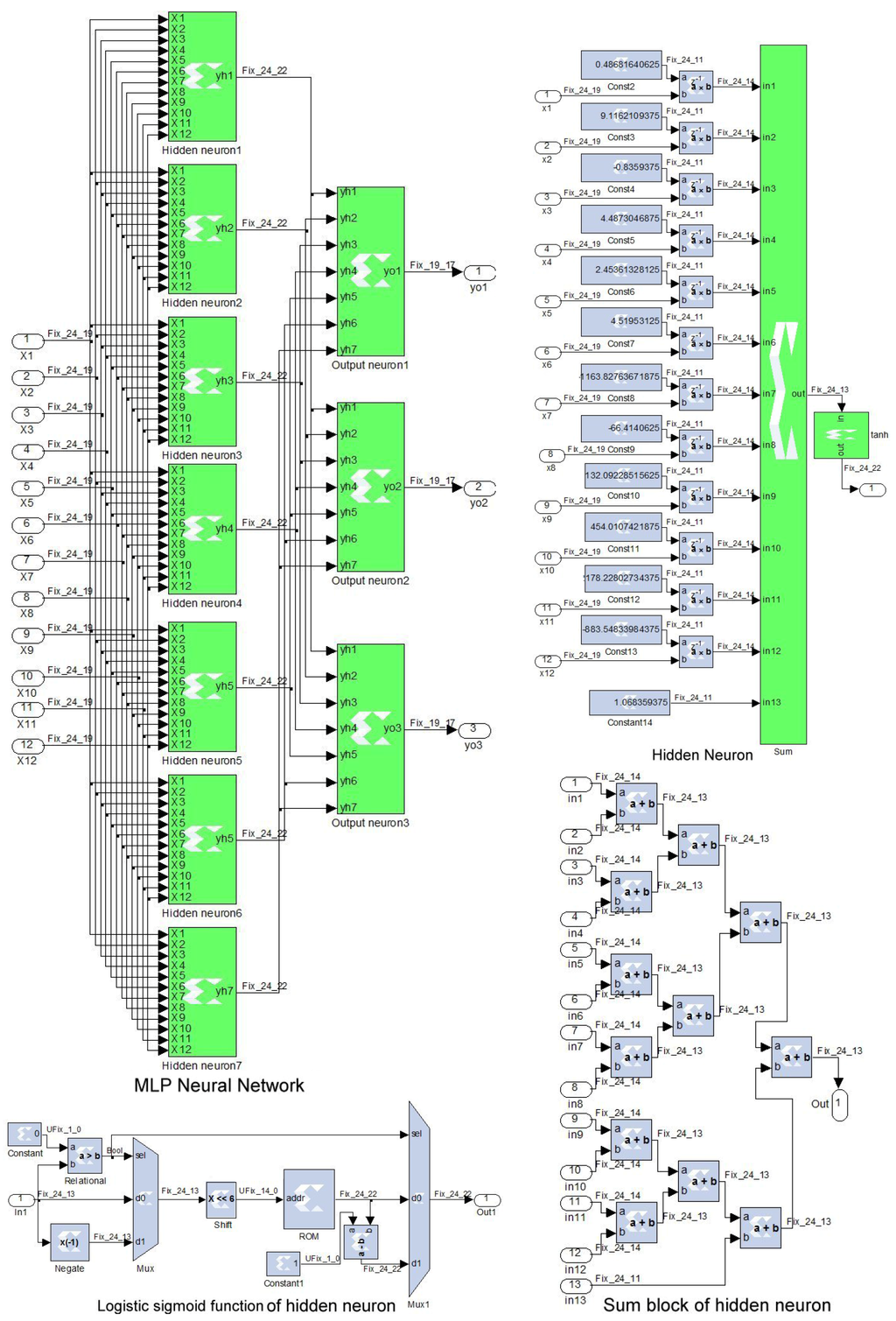
Figure 6.
Architecture of the implemented MLP neural network. The hidden neuron structure, and its sum and hyperbolic tangent blocks are also detailed.
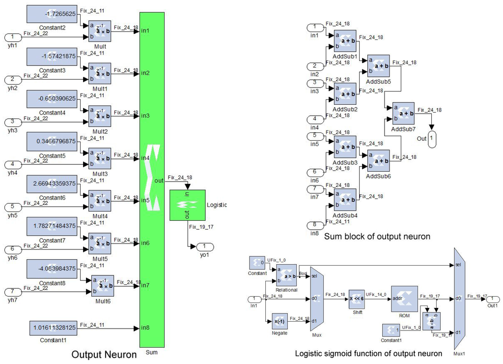
Figure 7.
Implementation of the output neuron and its sum and logistic sigmoid blocks.
3.7. Class Recognizer
For a vocalization of M frames presented to the system input, the class recognizer block compares the resulting neural network outputs to associate it to one of the predefined classes. As shown in Figure 8, the class recognizer uses an accumulator at each of the neural network outputs , , and that correspond to A, B, and D vocalization classes, respectively. Enabled by the ctrl signal, these accumulators compute the sums of the values obtained at these outputs during the M frames, according to Equation (11). Comparator and multiplexer blocks are used to find the index of the largest cumulated output among , , and , according to Equation (9). The recognized class is represented by integer values that correspond to A, B, and D vocalization classes, respectively.
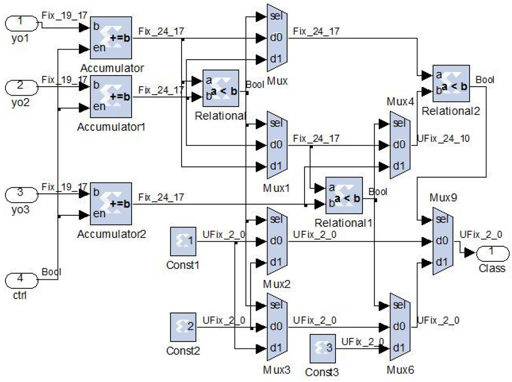
Figure 8.
Implementation of the class recognizer.
3.8. Implementation Characteristics
Starting with 36-bit fixed-point format in various blocks of the XSG-based model in order to ensure the same classification performance as the floating-point format of Matlab simulation, the data width was progressively reduced using a test-error approach. The fixed-point formats (generally of 24 bits) used in different blocks, that guarantee the same performance as Matlab, are shown in Figure 5, Figure 6, Figure 7 and Figure 8. For example, FIX_24_19 represents a 2’s complement signed 24-bit fixed-point format having 19 fractional bits. UFIX_24_10 represents an unsigned 24-bit fixed-point format having 10 fractional bits.
Once completed and verified, the XSG-based architecture can be automatically mapped to hardware implementation. Two FPGA chips are targeted in this study: Artix-7 XC7A100T and Virtex-6 XC6VLX240T available on the Nexys-4 and ML605 boards, respectively. Table 1 gives the resource utilization, the total power consumption, and the maximum operating frequency, as provided by the Xilinx ISE 14.7 tool. These values are based on the fixed-point data format and the ROMs size indicated on Figure 5, Figure 6, Figure 7 and Figure 8. The proposed architecture uses 219 DSP48E1s blocks. This is justified by the parallel architecture of the MLP networks that requires 12 multipliers for each hidden neuron and 7 multipliers for each output neuron. Thus, the MLP network requires 7 × 12 + 3 × 7 = 105 multipliers of numbers coded with 24 bits. The power spectrum block needs 2 multipliers of numbers coded with 26 bits, while the windowing block needs 1 multiplier of numbers coded with 16 bits. Considering the fact that each DSP48E1 slice contains one 25 × 18 multiplier, a multiplication of two numbers coded with 26-bit, 24-bit and 16-bit fixed-point format requires 4, 2 and 1 DSP48E1s, respectively. Therefore, the whole architecture requires 105 × 2 + 2 × 4 + 1 = 219 DSP48E1s. Except for DSP48E1s, this architecture requires only a small part of resources available on these FPGA (Artix-7 and Virtex-6). Difference in the maximum operating frequency is probably due to the speed grades of these FPGAs.
The implemented architecture on the Artix-7 XC7A100T FPGA operates at more than 25 MHz and consumes less than 123 mW. It can be an interesting solution for autonomous real-time classification system. The blue whale calls are sampled at 2 kHz.

Table 1.
Resource utilization, maximum operating frequency, and total power consumption obtained for the Artix-7 XC7A100T and Virtex-6 XC6VLX240T chips, as reported by the Xilinx ISE 14.7 tool. Each FPGA slice contains four LUTs (look-up tables) and eight flip-flops. Each DSP48E1 slice includes a 25 × 18 multiplier, an adder, and an accumulator.
| Targeted FPGA | Artix-7 XC7A100T | Virtex-6 XC6VLX240T | |
|---|---|---|---|
| Resource utilization | |||
| Slices | 6931 (of 15,850) | 7545 (of 37,680) | |
| Flip Flops | 13,330 (of 126,800) | 13,546 (of 301,440) | |
| LUTs | 21,658 (of 63,400) | 21,322 (of 150,720) | |
| Bonded IOBs | 20 (of 210) | 20 (of 600) | |
| RAMB18E1s | 2 (of 270) | 2 (of 832) | |
| DSP48E1s | 219 (of 240) | 219 (of 768) | |
| Maximum operating frequency | 25.237 MHz | 27.889 MHz | |
| Total power consumption | 0.123 W | 3.456 W | |
4. Experimental Results
4.1. Database
The recordings were collected in the Saguenay-St. Lawrence Marine Park at the head of the 300-m deep Laurentian channel in the Lower St. Lawrence Estuary. The used hydrophones were AURAL autonomous hydrophones (Multi-Electronique Inc., Rimouski, QC, Canada) moored at intermediate depths in the water column, as in standard oceanographic mooring. The 16-bit recording data were acquired at the 2000 Hz optional sampling rate of the AURALs, which includes an appropriate antialiasing low-pass filter of 1000 Hz [30]. For the blue whale calls classification, the selected recordings were down–sampled to 250 Hz [10,11].
4.2. Protocol
Blue whale vocalizations were extracted manually from records and categorized into the three classes (A, B and D) by the visualization of their spectrogram using Adobe Audition (1.5, Adobe, San Jose, CA, USA, 2004) software. Each class of the constructed database contains 100 calls. To use the whole dataset, the “k-fold cross-validation” method is employed to evaluate the performance of the implemented characterization/classification architecture. The principle of this method consists in dividing each class into 10 groups, each time we use 9 groups for training and the last one for the test [10,11].
4.3. Classification Performance
The performance of the proposed classifier is evaluated by the ratio of the number of the correctly classified vocalization (NCCV) to the number of tested vocalizations (NTV) [10,11].
4.4. Simulation Using XSG Blockset
This section presents the simulation results obtained with the proposed architecture implemented with XSG blockset (Figure 5, Figure 6, Figure 7 and Figure 8). These blocks provide bit and cycle accurate modeling for arithmetic and logic functions, memories, and DSP functions.
Figure 9 presents an A call input and its corresponding response signals obtained at different levels of the implemented characterization/classification architecture. The input signal is first split into non-overlapped frames using Hamming windows. The FFT block has an output latency of 1150 samples that corresponds to the delay between the first sample of a given input frame and the first sample of its Fourier transform . The power spectrum is computed for all the frequency components k of the frame m. As shown for , the feature vector components of a given frame m are updated at the end of this frame. The neural network outputs , and are calculated for each frame. The ctrl signal toggles high at the end of each of the proceeded M frames. There are only eight pulses because the length of this signal is greater than but less than , where N is the frame length of 512 samples. The class recognizer provides a provisory class index that is based on the neural network outputs of the present and the previous frames. The actual class recognition will be available only when the last frame is proceeded. The A call is classified as B during the first three frames, but is truly classified as A at the last frame (Figure 9). Figure 10 and Figure 11 present the same response signals but for B and D calls, respectively. Note that the B call (Figure 10) is confounded with the A call during the first four frames. However, the D call (Figure 11) is clearly separated from the A and B ones during all frames.
On the other hand, Figure 12 shows the feature vectors, the MLP neural network outputs, and the class recognizer output obtained for an A call. It can be seen that the first neural network output is globally predominant, but during the first three frames, the A call is confounded with the B call. Figure 13 and Figure 14 present the same response signals but for the B and D calls, respectively. Figure 13 shows that the second neural network output is globally predominant, but the B call is confounded with the A call during the first four frames. Figure 14 shows that the D call is clearly discriminated from the A and B calls during all frames. Note that A and B calls are principally represented by the first half of the feature components , while the D call is represented by the second half ones (Figure 12, Figure 13 and Figure 14).
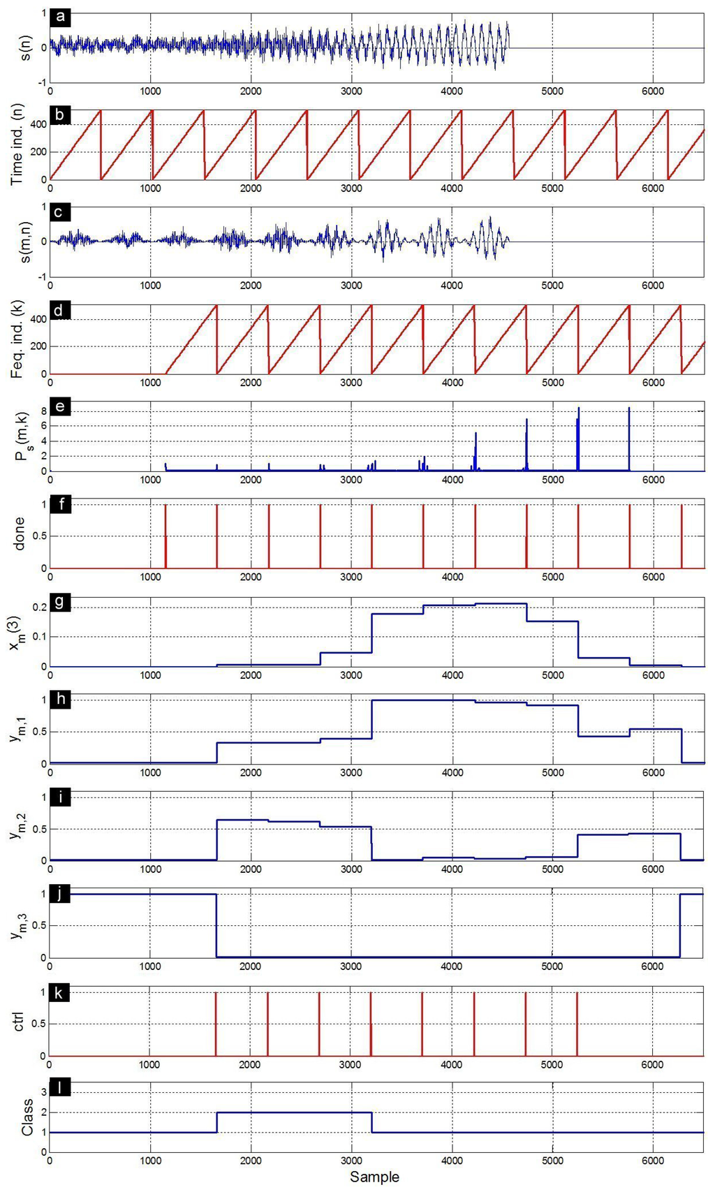
Figure 9.
Response signals obtained during the characterization/classification of an A call. (a) input signal ; (b) time index n that allows to delimit successive frames ; (c) windowed signal ; (d) frequency index k that allows to delimit successive power spectra; (e) power spectra ; (f) done signal; (g) third component of the feature vector ; (h) first MLP output ; (i) second MLP output ; (j) third MLP output ; (k) ctrl signal; and (l) recognized class.
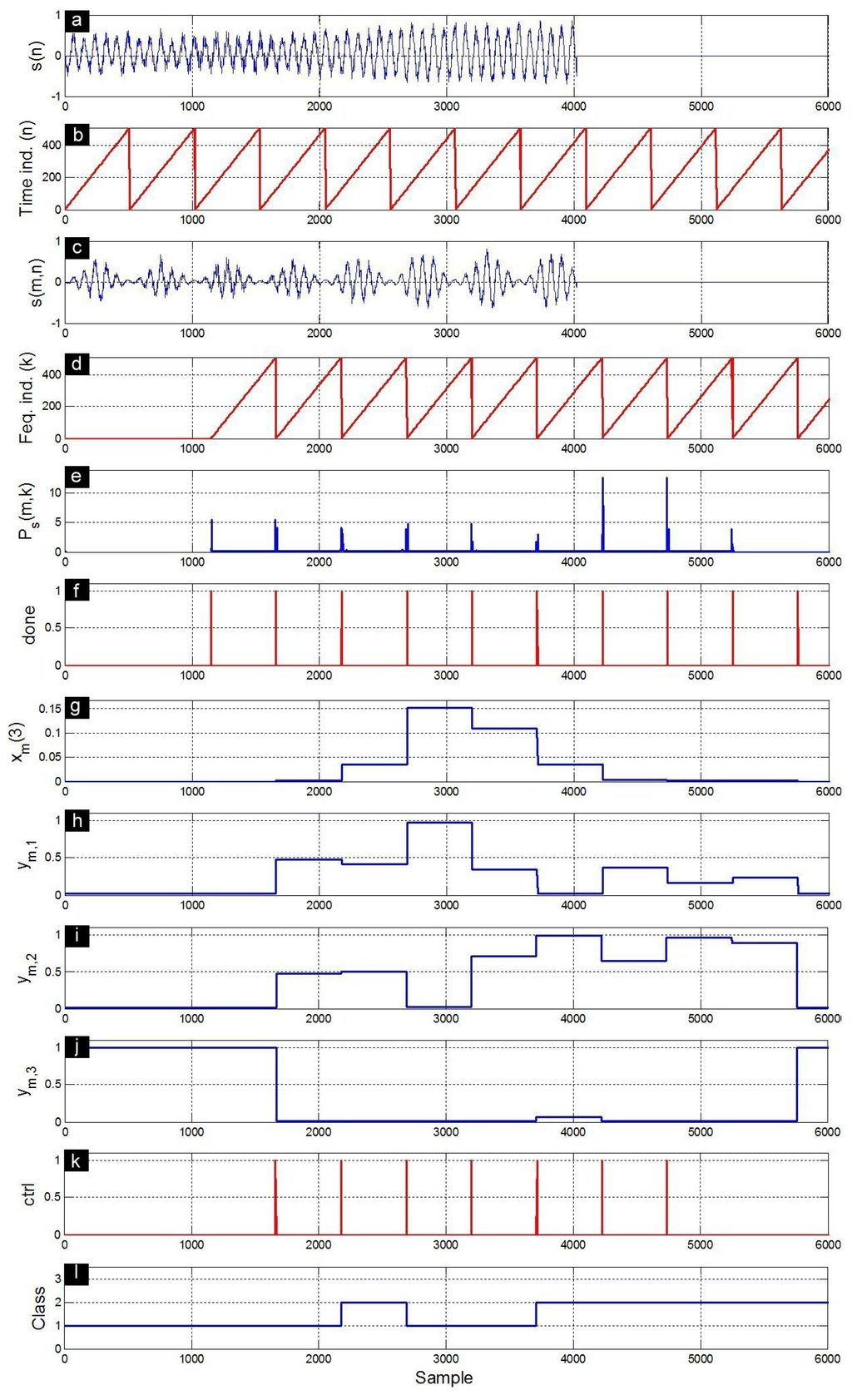
Figure 10.
Response signals obtained during the characterization/classification of a B call. (a) input signal ; (b) time index n that allows to delimit successive frames ; (c) windowed signal ; (d) frequency index k that allows to delimit successive power spectra; (e) power spectra ; (f) done signal; (g) third component of the feature vector ; (h) first MLP output ; (i) second MLP output ; (j) third MLP output ; (k) ctrl signal; and (l) recognized class.
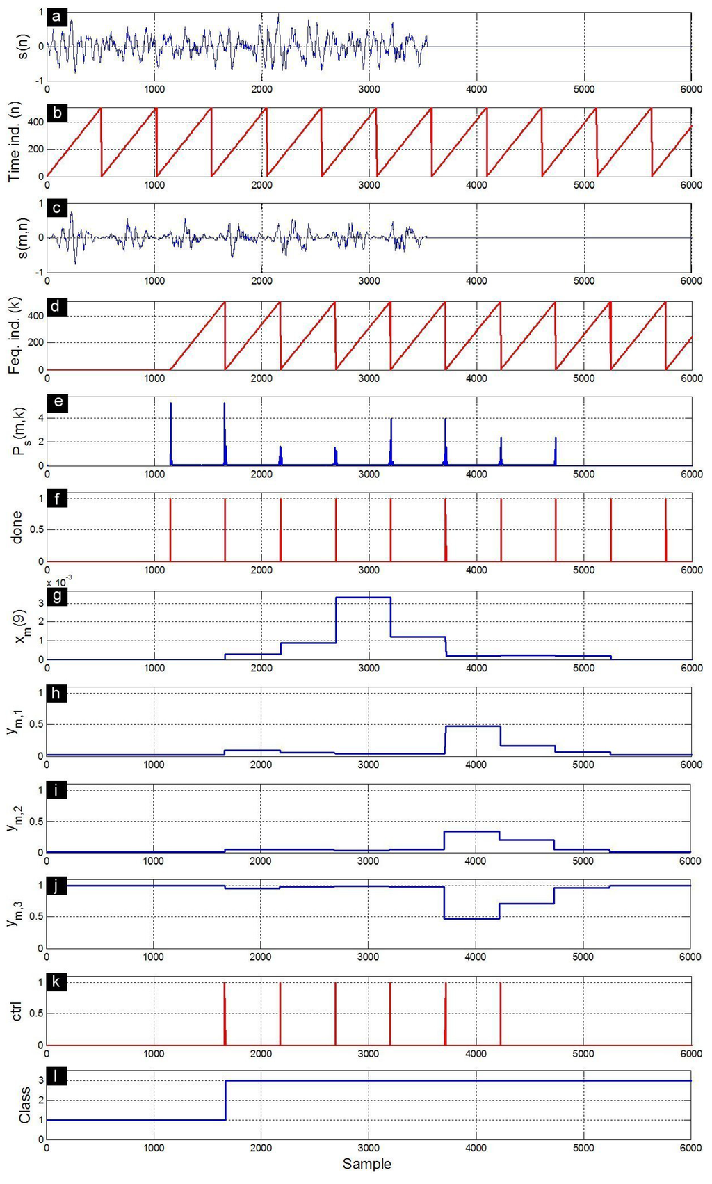
Figure 11.
Response signals obtained during the characterization/classification of a D call. (a) input signal ; (b) time index n that allows to delimit successive frames ; (c) windowed signal ; (d) frequency index k that allows to delimit successive power spectra; (e) power spectra ; (f) done signal; (g) ninth component of the feature vector ; (h) first MLP output ; (i) second MLP output ; (j) third MLP output ; (k) ctrl signal; and (l) recognized class.
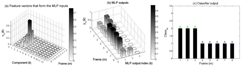
Figure 12.
(a) feature vectors based on STFT extracted from an A call; (b) MLP neural network outputs; and (c) class recognizer output. During the first three frames, the A call is confounded with B.
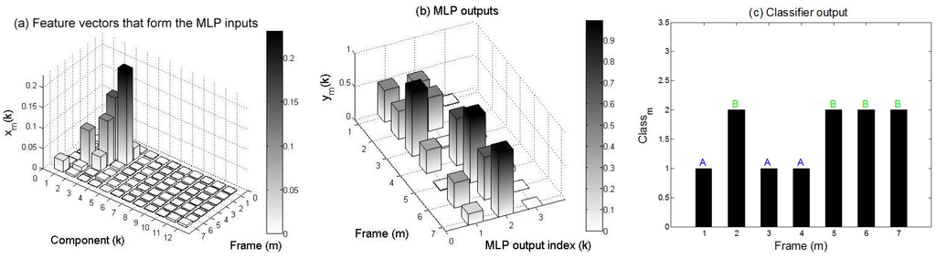
Figure 13.
(a) feature vectors based on STFT extracted from a B call; (b) MLP outputs; and (c) class recognizer output. During the first frames, the B call is confounded with A.
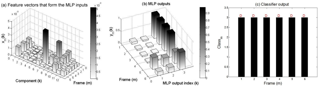
Figure 14.
(a) feature vectors based on STFT extracted from a D call; (b) MLP outputs; and (c) class recognizer output. Over all frames, the D call is discriminated from the A and B calls.
4.5. Hardware/Software Co-Simulation
The ML605 evaluation kit is pre-configured in the Simulink/XSG environment for hardware co-simulation. System Generator block allows us to choose a clock frequency target design of 33.3, 50, 66.7 or 100 MHz. However, the Nexys-4 board must be configured by the customer to achieve the hardware co-simulation. Once the designed model is verified by Simulink simulation using XSG blockset, it can be executed on actual FPGA using the hardware co-simulation compilation provided by the System Generator. Depending on the targeted board, this compilation automatically creates a bitstream and associated it to a Simulink block (Figure 15). When the design is simulated, the compiled model is executed in hardware with the flexible simulation environment of Simulink. System Generator reads the input data from wav file in Simulink environment and send them to the design on the board using the JTAG connection. It then reads the classification result (output) back from JTAG and sends it to Simulink for display.
Table 2 shows that the fixed-point XSG implementation gives the same performance (85.67%) as the floating-point Matlab one using the described database. Table 3 gives the confusion matrix of the true classes versus assigned classes for the fixed-point and floating-point implementations of the STFT/MLP based classifier. These results show the high performance of the implemented method to separate D class from A and B, but its difficulty to discriminate A and B classes [10]. The obtained classification result (85.67%) with only 7 hidden neurons is comparable to that (86.25%) obtained with 25 hidden neurons [10]. This slight difference can also be explained by other experimental test conditions : (a) the feature vectors are extracted with 0% overlap instead of 50%; (b) the use of logistic sigmoid in hidden layer instead of hyperbolic tangent; and (c) performance is obtained from one test instead of averaged values of 50 repeated tests [10].
It can be noted that the classification error between the fixed-point XSG implementation and the floating-point Matlab simulation will not be zero if the data width is not sufficient. This error will increase if the number of bits decreases under the values indicated in Figure 5, Figure 6, Figure 7 and Figure 8.
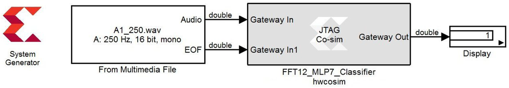
Figure 15.
Simulink diagram of the hardware/software cosimulation.
Table 2.
Performances obtained with XSG and Matlab based implementations.
| Vocalization | Performance (%) | |
|---|---|---|
| XSG | Matlab | |
| A | 79 | 79 |
| B | 82 | 82 |
| D | 96 | 96 |
| Total | 85.67 | 85.67 |
Table 3.
Confusion matrix of XSG and Matlab based implementations.
| True Class | Assigned Class (XSG) | Assigned Class (Matlab) | |||||
|---|---|---|---|---|---|---|---|
| A | B | D | A | B | D | ||
| A | 79 | 18 | 3 | 79 | 18 | 3 | |
| B | 16 | 82 | 2 | 16 | 82 | 2 | |
| D | 0 | 4 | 96 | 0 | 4 | 96 | |
5. Conclusions
A blue whale calls classification technique based on short-time Fourier transform and MLP neural network has been successfully implemented on FPGA using a high-level programming language (XSG). The fixed-point XSG implementation, on the low-cost Nexys-4 Artix-7 FPGA board, provides the same classification performance as the floating-point Matlab simulation using a reduced number of bits. The maximum operating frequency and the total power consumption obtained for the Artix-7 XC7A100T FPGA show that the proposed architecture can be used to build an autonomous real-time classification system.
As future work, a vocalization activity detector (VAD) will be added to automatically extract the calls before there classification.
Acknowledgments
The author gratefully acknowledge the Natural Sciences and Engineering Research Council of Canada (NSERC). He would like to thank Dr. Yvan Simard from the Marine Sciences Institute of the Université du Québec à Rimouski for fruitful discussions and proof reading.
Conflicts of Interest
The author declares no conflict of interest.
References
- Chen, C.; Lee, J.; Lin, M. Classification of underwater signals using wavelet transforms and neural networks. Mathe. Comput. Model. 1998, 27, 47–60. [Google Scholar]
- Huynh, Q.; Cooper, L.; Intrator, N.; Shouval, H. Classification of underwater mammals using feature extraction based on time-frequency analysis and bcm theory. IEEE Trans. Signal Process. 1998, 46, 1202–1207. [Google Scholar] [CrossRef]
- Deecke, V.; Ford, J.; Spong, P. Quantifying complex patterns of bioacoustic variation: Use of a neural network to compare killer whale (Orcinus orca) dialects. J. Acoust. Soc. Am. 1999, 105, 2499–2507. [Google Scholar] [CrossRef] [PubMed]
- Chesmore, E. Application of time domain signal coding and artificial neural networks to passive acoustical identification of animals. Appl. Acoust. 2001, 62, 1359–1374. [Google Scholar] [CrossRef]
- Chesmore, E.; Ohya, E. Automated identification of field-recorded songs of four British grasshoppers using bioacoustic signal recognition. Bull. Entomol. Res. 2004, 94, 319–330. [Google Scholar] [CrossRef] [PubMed]
- Reby, D.; André-Obrecht, R.; Galinier, A.; Farinas, J.; Cargnelutti, B. Cepstral coefficients and hidden Markov models reveal idiosyncratic voice characteristics in red deer (Cervus elaphus) stags. J. Acoust. Soc. Am. 2006, 120, 4080–4089. [Google Scholar] [CrossRef] [PubMed]
- Van Der Schaar, M.; Delory, E.; Català, A.; André, M. Neural network-based sperm whale click classification. J. Mar. Biol. Assoc. UK 2007, 87, 35–38. [Google Scholar] [CrossRef]
- Roch, M.; Soldevilla, M.; Burtenshaw, J.; Henderson, E.; Hildebrand, J. Gaussian mixture model classification of odontocetes in the Southern California Bight and the Gulf of California. J. Acoust. Soc. Am. 2007, 121, 1737–1748. [Google Scholar] [CrossRef] [PubMed]
- Mouy, X.; Bahoura, M.; Simard, Y. Automatic recognition of fin and blue whale calls for real-time monitoring in the St. Lawrence. J. Acoust. Soc. Am. 2009, 126, 2918–2928. [Google Scholar] [CrossRef] [PubMed]
- Bahoura, M.; Simard, Y. Blue Whale Calls Classification using Short-Time Fourier and Wavelet Packet Transforms and Artificial Neural Network. Digit. Signal Process. 2010, 20, 1256–1263. [Google Scholar] [CrossRef]
- Bahoura, M.; Simard, Y. Serial combination of multiple classifiers for automatic blue whale calls recognition. Expert Syst. Appl. 2012, 39, 9986–9993. [Google Scholar] [CrossRef]
- Mielke, A.; Zuberbühler, K. A method for automated individual, species and call type recognition in free-ranging animals. Anim. Behav. 2013, 86, 475–482. [Google Scholar] [CrossRef]
- Adam, O.; Samaran, F. Detection, Classification and Localization of Marine Mammals Using Passive Acoustics. 2003–2013: 10 Years of International Research; Dirac NGO: Paris, France, 2013. [Google Scholar]
- Kershenbaum, A.; Roch, M. An image processing based paradigm for the extraction of tonal sounds in cetacean communications. J. Acoust. Soc. Am. 2013, 134, 4435–4445. [Google Scholar] [CrossRef] [PubMed]
- Au, W.; Hastings, M. Principles of Marine Bioacoustics; Springer: New York, NY, USA, 2008. [Google Scholar]
- Simard, Y.; Roy, N.; Gervaise, C. Passive acoustic detection and localization of whales: Effects of shipping noise in Saguenay-St. Lawrence Marine Park. J. Acoust. Soc. Am. 2008, 123, 4109–4117. [Google Scholar] [CrossRef] [PubMed]
- Simard, Y.; Roy, N. Detection and localization of blue and fin whales from large-aperture autonomous hydrophone arrays: A case study from the St. Lawrence estuary. Can. Acoust. 2008, 36, 104–110. [Google Scholar]
- Ortigosa, E.M.; Cañas, A.; Ros, E.; Ortigosa, P.M.; Mota, S.; Díaz, J. Hardware description of multi-layer perceptrons with different abstraction levels. Microprocess. Microsyst. 2006, 30, 435–444. [Google Scholar] [CrossRef]
- Armato, A.; Fanucci, L.; Scilingo, E.; Rossi, D.D. Low-error digital hardware implementation of artificial neuron activation functions and their derivative. Microprocess. Microsyst. 2011, 35, 557–567. [Google Scholar] [CrossRef]
- Manikandan, J.; Venkataramani, B. Design of a real time automatic speech recognition system using Modified One Against All SVM classifier. Microprocess. Microsyst. 2011, 35, 568–578. [Google Scholar] [CrossRef]
- Wang, J.; Wang, J.F.; Weng, Y. Chip design of MFCC extraction for speech recognition. Integr. VLSI J. 2002, 32, 111–131. [Google Scholar] [CrossRef]
- Amudha, V.; Venkataramani, B. System on programmable chip implementation of neural network-based isolated digit recognition system. Int. J. Electron. 2009, 96, 153–163. [Google Scholar] [CrossRef]
- Staworko, M.; Rawski, M. FPGA implementation of feature extraction algorithm for speaker verification. In Proceeding of the 17th International Conference “Mixed Design of Integrated Circuits and Systems”, MIXDES 2010, Warsaw, Poland, 24–26 June 2010; pp. 557–561.
- Ramos-Lara, R.; López-García, M.; Cantó-Navarro, E.; Puente-Rodriguez, L. Real-Time Speaker Verification System Implemented on Reconfigurable Hardware. J. Signal Process. Syst. 2013, 71, 89–103. [Google Scholar] [CrossRef] [Green Version]
- Pan, S.; Lan, M. An efficient hybrid learning algorithm for neural network-based speech recognition systems on FPGA chip. Neural Comput. Appl. 2013, 24, 1–7. [Google Scholar] [CrossRef]
- Hoang, T.; Truong, N.; Trang, H.; Tran, X. Design and Implementation of a SoPC System for Speech Recognition. In Multimedia and Ubiquitous Engineering; Park, J., Ng, J., Jeong, H., Waluyo, B., Eds.; Springer: New York, NY, USA, 2013; Volume 240, pp. 1197–1203. [Google Scholar]
- Lin, B.S.; Yen, T.S. An FPGA-based rapid wheezing detection system. Int. J. Environ. Res. Public Health 2014, 11, 1573–1593. [Google Scholar] [CrossRef] [PubMed]
- Haykin, S. Neural Networks: A Comprehensive Foundation, 2nd ed.; Prentice-Hall: Upper Saddle River, NJ, USA, 1999. [Google Scholar]
- Bahoura, M.; Ezzaidi, H. FPGA implementation of a feature extraction technique based on Fourier transform. In Proceeding of the 24th International Conference on Microelectronics (ICM), Algiers, Algeria, 16–20 December 2012; pp. 1–4.
- Simard, Y.; Bahoura, M.; Roy, N. Acoustic Detection and Localization of whales in Bay of Fundy and St. Lawrence Estuary Critical Habitats. Can. Acoust. 2004, 32, 107–116. [Google Scholar]
© 2016 by the author; licensee MDPI, Basel, Switzerland. This article is an open access article distributed under the terms and conditions of the Creative Commons by Attribution (CC-BY) license (http://creativecommons.org/licenses/by/4.0/).