1. Introduction
The radio spectrum is a precious resource that needs careful planning, as the currently licensed spectrum is severely underutilized [
1]. Cognitive radio (CR) [
2], which adapts the radio’s operating characteristics to the real-time conditions, is the key technology that allows flexible, efficient and reliable spectrum utilization to be realized in wireless communications. This technology exploits the facts that the licensed spectrum is underutilized by the primary user(s) (PU), and it introduces the secondary user(s) (SU) to operating on the spectrum that is either opportunistically available or concurrently being shared by the PU and SU. The proposed paper focuses on the latter case.
Since the multiple-input multiple-output (MIMO) technology uses multiple antennas at both the transmitter and the receiver to significantly increase data throughput and link range without additional bandwidth or transmit power, it plays an important role in wireless communications today.
The works in [
3,
4,
5] set up some algorithms to compute the maximum sum-rate problems for the Gaussian broadcast channel and the sum-power constrained Gaussian dual multiple-access channel. In addition, for computing the maximum weighted sum-rate for a class of the Gaussian SIMO (single-input-multiple-output) systems, [
6] has also presented some algorithms to provide the max-stability policy. Those meaningful works are applied to the non-CR networks. For the SIMO-MAC in CR networks, as a special case of the MIMO-MAC in CR networks, the weighted sum-rate maximization problem has been investigated in [
7] to compute the optimal power allocation. In the recent published papers [
8,
9], the MAC protocol identification and the joint subcarrier and bit allocation issues under CR networks were discussed, respectively. On spectrum sensing of CR, there are some meaningful works, such as [
10] and the references cited therein.
In this paper, we integrate the CR networks with MIMO technology to fully ensure the quality of service (QoS) of PUs, as well as to maximize the sum-rate of SUs. Since multiple-antenna mobile users are quite common due to the efficiency of the mobile terminals, we simply term this setting as a multiple input multiple output multiple access channel (MIMO-MAC) in CR networks and confine the topic to the MIMO-MAC situation. We set up more practical mathematical models for the target problem. In addition, with the added constraints, conventional water-filling algorithms cannot be used due to a more complicated problem structure. By exploiting the structure of the sum-rate optimization problem, we propose a dual decomposition algorithm based on the water-filling principle to compute the optimal allocation distribution and the maximum sum-rate.
The proposed algorithm owns several improvements, shown below. First, to avoid ineffectively using the dual decomposition algorithm and to make the proposed algorithm more efficient, a tight pair of upper and lower bounds, as an interval for the optimal Lagrange multiplier, is proposed. Especially when the number of the users is sufficiently large, the benefits of utilizing this interval can be significant.
Second, we reduce the sum-rate problem into solving a decoupled system. Each block of the decoupled system can be solved by a highly efficient water-filling-like algorithm, due to the characteristics of both the objective function and the decoupled constraint system, with each of the blocks solved by the water-filling-like algorithm.
Moreover, the convergence of the proposed algorithm can be guaranteed through the rigorous mathematical proof presented in this paper. As a result, the proposed algorithm offers fast convergence. It is important to note that the convergence of the proposed algorithm is based on the theoretical advances from the fundamental results of the previously-mentioned acclaimed papers. In particular, the proposed approach overcomes the limitation of Hermitian matrices as independent variables. This limitation to the optimization problem in several complex variables has not been well investigated in the open literature. The existing optimization theory and methods, including the convex optimization theory and methods, deal with the problems with the optimization variables in the real
n-dimensional Euclidean space (refer to [
11,
12,
13]), but not in the complex
n-dimensional unitary space. The target problem falls into the latter category. As a result, our analysis and results are solidly extended to the field of complex numbers, which are more compatible with practical communication systems.
Key notations that are used in this paper are as follows: |
A| and Tr (
A) give the determinant and the trace of a square matrix
A, respectively;
A ⪰ 0 means that the matrix
A is positive-semidefinite;
E[
X] is the expectation of the random variable
X; the capital symbol
I for a matrix denotes the identity matrix with an appropriate size; in addition, for any complex matrix, its superscript † denotes the conjugate transpose of the matrix. Some notations or symbols are listed in
Table 1.
Table 1.
List of variables and abbreviations. SU, secondary user.
Table 1.
List of variables and abbreviations. SU, secondary user.
| Variables & Abbreviations | Representations or Interpretations |
|---|
| k* | water level step (highest step under water) |
| E | expectation on probability |
| K | total number of channels |
| Pt | upper bound for total power or sum-power |
| Pk | upper bound for the peak power constraint at step k |
| Tr | trace operation of a square matrix |
| xi | signal transmitted by the i-th SU, which is a column vector |
| Si | E[xi(xi)†], which is a matrix |
| λ | Lagrange multiplier or dual variable |
2. MIMO-MAC in a CR Network and Its Sum-Rate
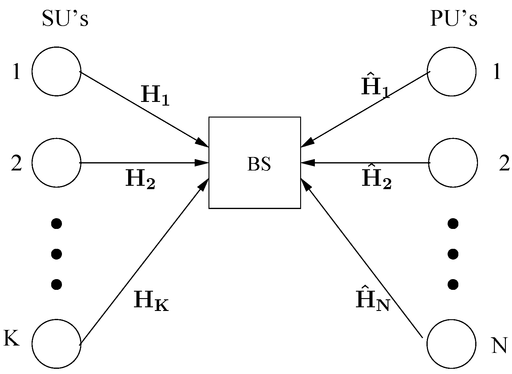
For the MIMO-MAC in CR networks, assume that there is one base-station (BS) with
Nr antennas,
K SUs and
N PUs, each of which is equipped with
Nt antennas. In this section, assume that the MIMO-MAC under the CR network is described as:
are the given fixed channel matrices of SUs and PUs, respectively. As general assumptions, the signal
is a complex input signal vector from the
i-th SU, and it is a Gaussian random vector having zero mean with independent entries; and the signal
is a complex input signal vector from the
j-th PU, and it is a Gaussian random vector having zero mean with independent entries. Further,
is an additive Gaussian noise random vector,
i.e.,
. Thus,
is the received signal at the BS. Furthermore,
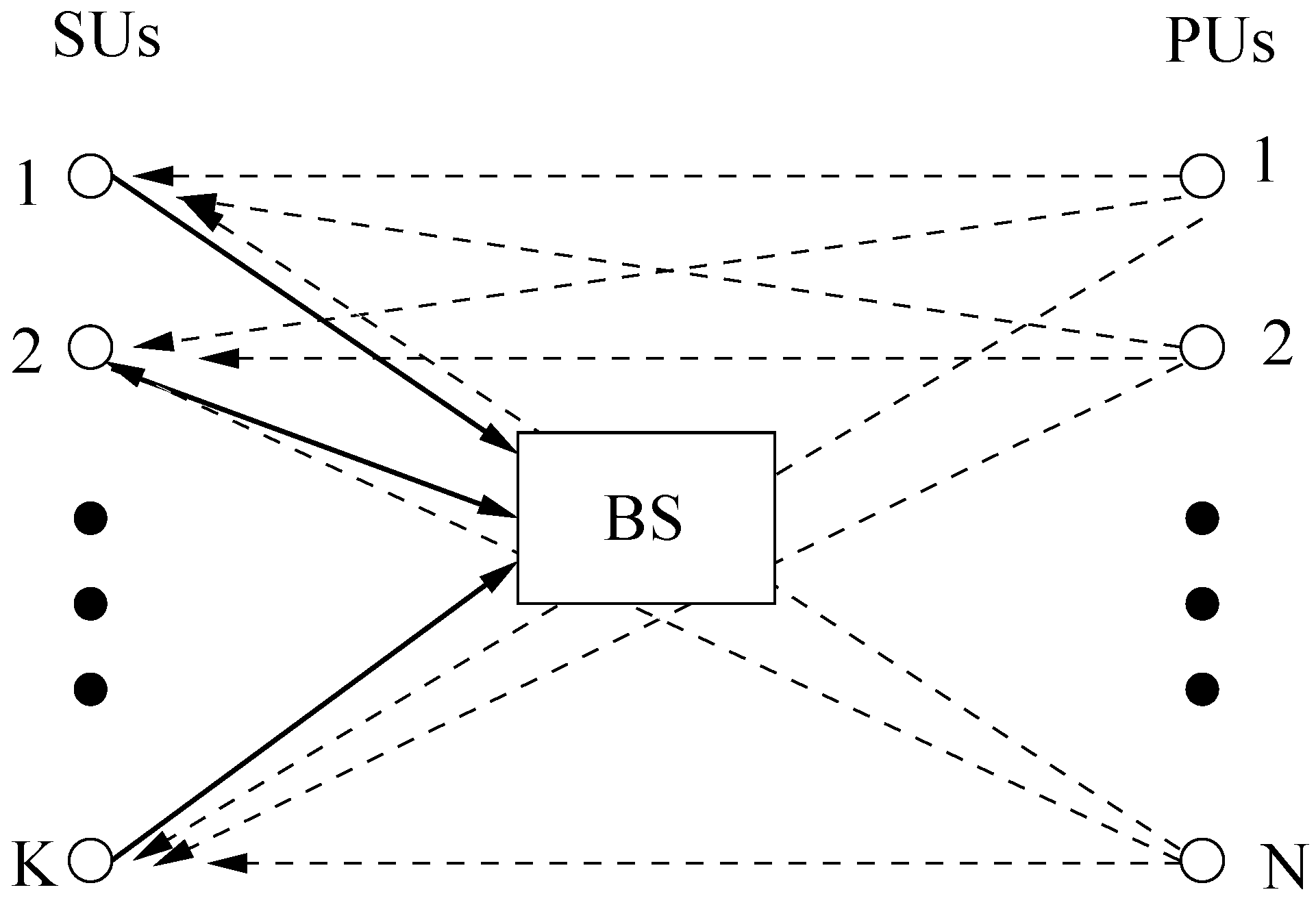
The MIMO-MAC in the CR network is illustrated in
Figure 1.
Figure 1.
Cognitive radio (CR)-MIMO-MAC system model.
Figure 1.
Cognitive radio (CR)-MIMO-MAC system model.
To clarify the role of the transmitted signals from the SUs to the BS (represented by the thick solid lines), with the transmitted signal from the PUs to the BS playing the role of the interference to the SUs (represented by the dashed lines), it is illustrated in
Figure 2.
Figure 2.
SUs to BS and signals from primary users (PUs) as the interference.
Figure 2.
SUs to BS and signals from primary users (PUs) as the interference.
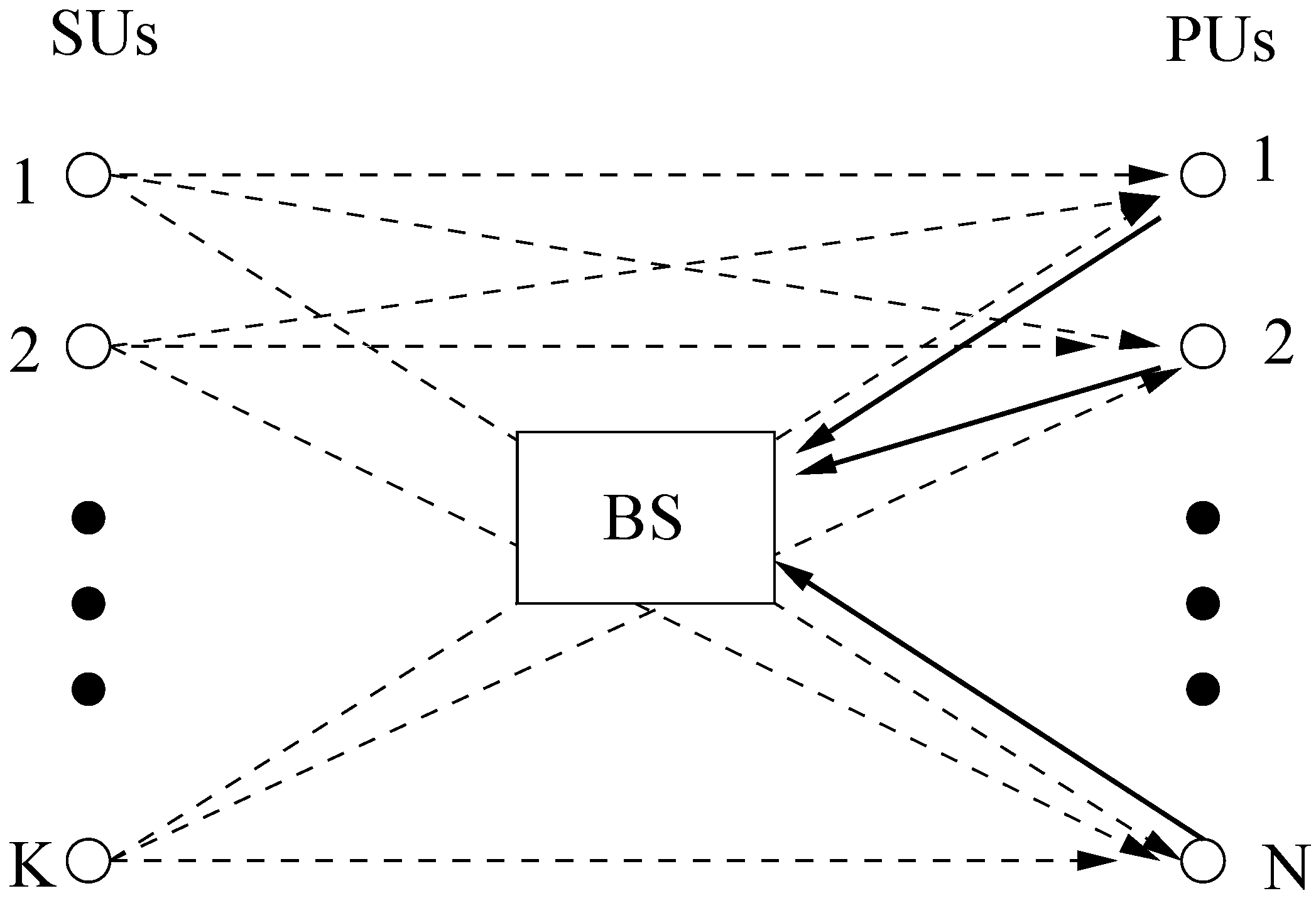
Figure 3 illustrates the case when the roles are exchanged between the SUs and PUs.
Figure 3.
PUs to BS and signals from SUs as the interference.
Figure 3.
PUs to BS and signals from SUs as the interference.
The mathematical model of the sum-rate optimization problem for the MIMO-MAC in the CR network can be written as follows:
where the upper bound of the peak power constraint on the
i-th SU is denoted by
Assume
and
for any
i. Further, without loss of generality,
is assumed to have the identity covariance matrix in the model (3).
The constraint:
of the sum-rate optimization problem (3) of the MIMO-MAC in the CR network is called the sum-power constraint with gains. The gains denoted by
are defined as follows. Let:
where
is the additive interference and noise of the transmitted signal
, which is transmitted to the BS. To guarantee the QoS for PUs, the power of the interference and noise is less than the transmitted power by PUs. That is to say, setting up a threshold
Pt limits the transmitted power by the SUs and guarantees the QoS for PUs. The ratio of the threshold
Pt to the power used by PUs can be determined (for example, refer to [
14]).
Its mathematical expression can be expressed as:
i.e.,
Let
gk be the maximum eigenvalue of
Then, we only need:
such that Equation (6) holds. Thus, an innovation in our model is that we can construct the parameters
from the channel gain matrix and is referred to as the gains of the sum-power constraint. Let:
where the symbol “⇐” means the assignment operation, and
Pt is called the upper bound of the sum-power constraint with the gains.
Further, based on the same principle, a better transmission throughput model can also be obtained. Our approach reflects the essence of the target problem more practically.
In addition, assume that and . This case corresponds to the SIMO-MAC case in the CR networks.
Applying the QR decomposition,
H =
QR. Let
has orthogonal and normalized column vectors.
is an upper triangle matrix with
denoting the (
m,
k)-th entry of the matrix
R.
Q† is regarded as an equalizer to the received signal by the BS.
Thus, the
i-th SU should have the rate:
where
and
For easy processing, the third term in the denominator above has been ignored in some earlier works.
Extending the separating hyperplane theorem [
11] in convex optimization theory over the field of real numbers, or the direct product of the fields of real numbers to that over the field of complex numbers, or the direct product of the fields of complex numbers, we may obtain the following proposition.
Proposition 1. The optimization problem (3) is equivalent to the following optimization problem:i.e., the optimal objective values of the optimization problems (3) and (12) are equal. Furthermore, with the exception of the part of the dual variable, the restriction of any optimal solution of (12) (to the part of the original variable) is the same as the optimal solution of (3). Further, the optimal solution, λ*, to (12) is the optimal dual variable of the sum power constraint with gains in (3). 3. Algorithm ALW1
To efficiently solve the optimization problem (12), a new method is proposed as follows.
Given
λ ≥ 0 and the optimization problem:
an efficient iterative algorithm is proposed here, and the optimal objective function value for the problem (13) is denoted by
g(
λ). It is seen that
g(
λ) is a convex function over
λ ≥ 0, and
λ is a scalar. Thus, we may use the sub-gradient algorithm or a line search to obtain the optimal solution
λ* to the problem (12). Since the range to search is important, a pair of upper and lower bounds are proposed as follows.
Proposition 2. For the optimization problem (12), the optimal solution: Proof of Proposition 2. Since the optimization problems (3) and (12) are equivalent, for given
λ*, the latter is further transformed into the following problem:
to find the solution to (3), where the matrix diag
, with
being decreasingly ordered, is equivalent to the matrix
, under the meaning of the unitary similarity transformation by a unitary matrix
U. We have the KKTcondition:
where the optimal dual variable
and
k*(
k) is the highest step under the water during the steps from (
k − 1)
Nt to
kNt. From the properties of positive semi-definite matrices and the definitions of
and
gk, it is seen that
. Thus,
implies
λ* ≤ 1.
Therefore, Proposition 2 is proven.
The tightness of the interval means that there exists a set of channel gains, such that its optimal Lagrange multiplier λ* touches either of the ends of the interval. For example, as and h1 = 1, it is seen that λ* = 0.
Letting
λ ∈ (0, 1], consider the evaluation of
g(
λ). Note that the problem (13) has decoupled constraints. Therefore, the block coordinate ascend algorithm (BCAA) or the cyclic coordinate ascend algorithm (CCAA) (see [
12,
15]) can be used to solve the problem efficiently. The iterative algorithm works as follows. In each step, the objective function is maximized over a single matrix-valued variable
Sk, while keeping all other
Sks fixed,
and then repeating this process. Since the objective is nondecreasing with each iteration, the algorithm must converge to a fixed point. Using the fixed point theory, the fixed point is an optimal solution to the problem (13). Without loss of generality, let us consider an optimization problem with the optimization variable
Sk,
k = 1, with respect to all other
Sks being fixed, as follows:
It is known that gi > 0 due to Hi ≠ 0, ∀i. Note that the single user case above with respect to the fixed other users is different from the existing ones for the MIMO-MAC cases, since it has a more complicated objective or feasible set. However, we can still exploit the water-filling-like approach to solve (18). The skeleton is stated as follows.
An optimal solution to (18) can be computed by exploiting the water-filling-like approach (refer to [
16,
17] and the references therein), since the problem (18) is equivalent to the following problem.
where the mentioned
. Similarly, the problem (19) can be equivalent to the problem (20) below,
similarly, where the matrix diag
, with
being decreasing ordered, is equivalent to the matrix
, under the meaning of the unitary similarity transformation by a unitary matrix
U. It is seen that we can use a similar method to the water-filling-like approach [
18] to compute the optimal solution
to the problem (20) and then obtain the optimal solution
U diag
to the problem (18).
How to compute the optimal solution to the problem (20) is concisely and uniquely proposed as follows: if , then ; if , then . Further, if , such that , . Thus, under the condition mentioned above, if , then ; and . Else if , then , for ; and , for .
For
λ and the given
, the BCAA is used from the first matrix-valued variable to the
K-th variable, and we obtain:
Thus, a mapping can be defined, which projects:
This mapping is denoted by
f.
With the assumptions and the concepts introduced, a new iterative water-filling-like algorithm, ALW1, is concisely proposed as follows.
Algorithm ALW1:
- (1)
Given
, initialize:
- (2)
Set
- (3)
Then, . Repeat Procedure (3) mentioned until the optimal solution to the problem (13) is reached.
- (4)
If , then λmin is assigned by λ;
if , then λmax is assigned by λ;
if , stop.
- (5)
If , stop. Otherwise, go to Step (2)
Note that the initial
λmin is chosen as zero, and
λmax is chosen as one, respectively. If the initial values
λmin ≥ 0 and
λmax ≥ 0 are chosen as two points outside of the available range of the
λ*, there exists an example to account for the fact that algorithms via the dual decomposition principle cannot find any optimal solution. In Step (4) of ALW1, it is not difficult to see that
is a subgradient of the function
g(
λ). This is because:
where
is the optimal solution to (3).
According to the definition of the subgradient, is a subgradient of the function g(λ), although g(λ) cannot be guaranteed to be differential. Thus, we can follow the subgradient algorithm to search better λ in the Step (4) mentioned.
Example 1. and , the problem (13) is instanced as follows.
Let the initials and .
Dual decomposition algorithms cannot be used to find any optimal solution to this sum-rate maximization problem.
Therefore, from Example 1, it is easily seen that without proper initial values of λmin and λmax, it might result in the ineffectiveness and/or the inefficiency of a class of primal-dual algorithms with the subgradient approach.
4. Convergence of Algorithm ALW1
First, we will prove that for the fixed λ, the iterative water-filling can compute an optimal solution to the optimization problem (18).
Proposition 3. Via the proposed water-filling-like algorithm with a fixed λ, an optimal solution can be found to the optimization problem (18).
This proposition can be proven by the KKT condition [
12] of the optimization problem (18) and a similar method in [
18].
Second, convergence for the algorithm ALW1 is discussed as follows.
Theorem 1. For the optimal power allocation problem (3), ALW1 is convergent, following Proposition 3.
Proof. Due to construction of the tight interval or bounds for the optimal Lagrange multiplier
λ*, the convexity of both the optimization problems (12) and
g(
λ) and characteristic of the sub-gradient method, the Lagrange multiplier obtained by the iterations of the outer loop computation can approximate to
λ* only when the inner loop can guarantee convergence. It is seen that the cyclic coordinate ascent algorithm [
15] is used by the inner loop computation, and it is convergent if the solved problem is a convex optimization problem with a compact Cartesian direct product set as the feasible set and a continuously differential objective function for each of (15). The problem (3) can guarantee the conditions mentioned above. Therefore, ALW1 is convergent. ☐
5. Performance Results and Comparison
In this section, some numerical examples to illustrate the effectiveness of the proposed algorithm are presented. Since there is no existing method to compute the maximum sum-rate of the MIMO MAC in the CR networks, we made some development to the iterative water-filling-like algorithm in [
6] to solve the target problem for comparison purposes. This algorithm is referred to as Algorithm AW in this paper.
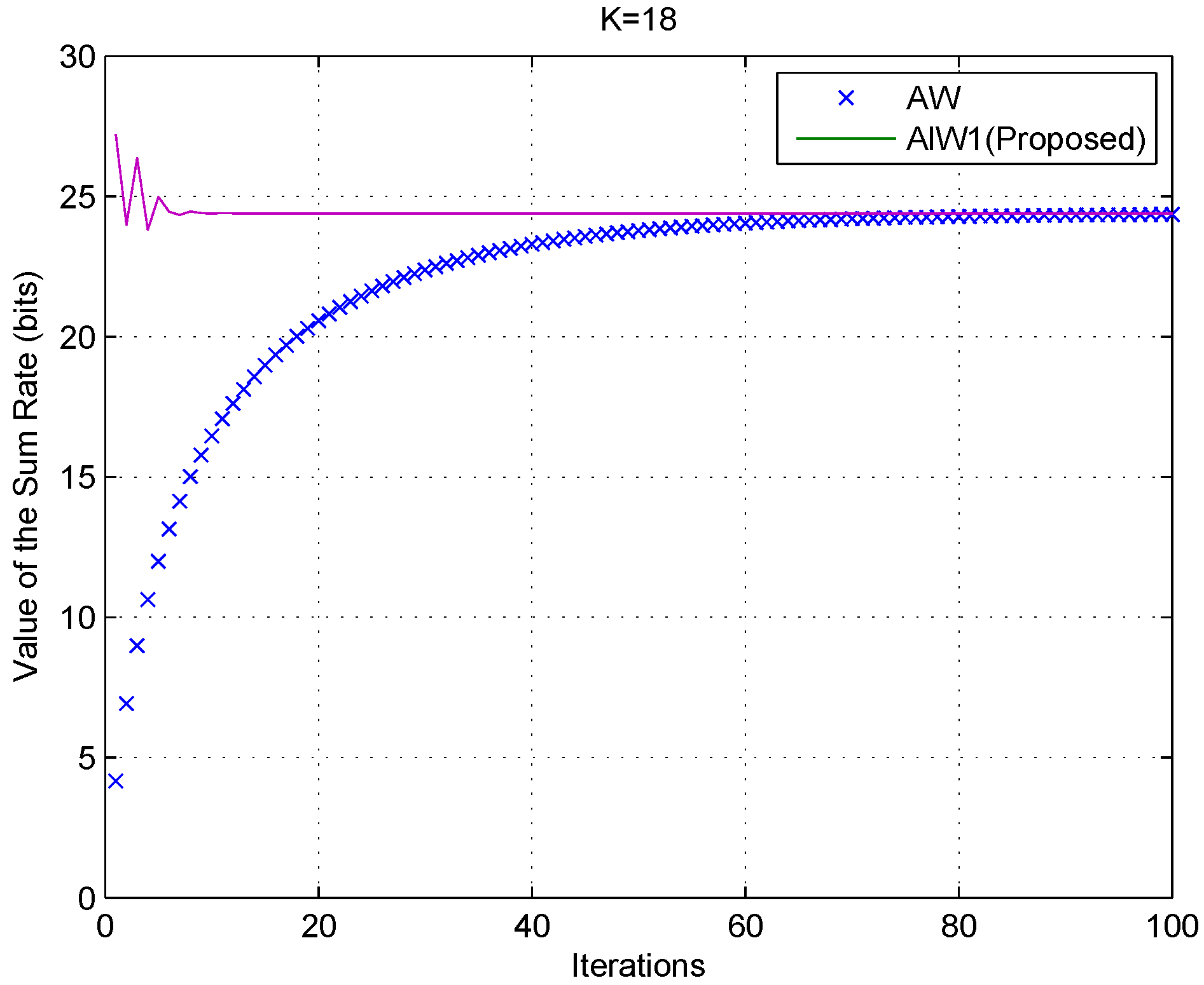
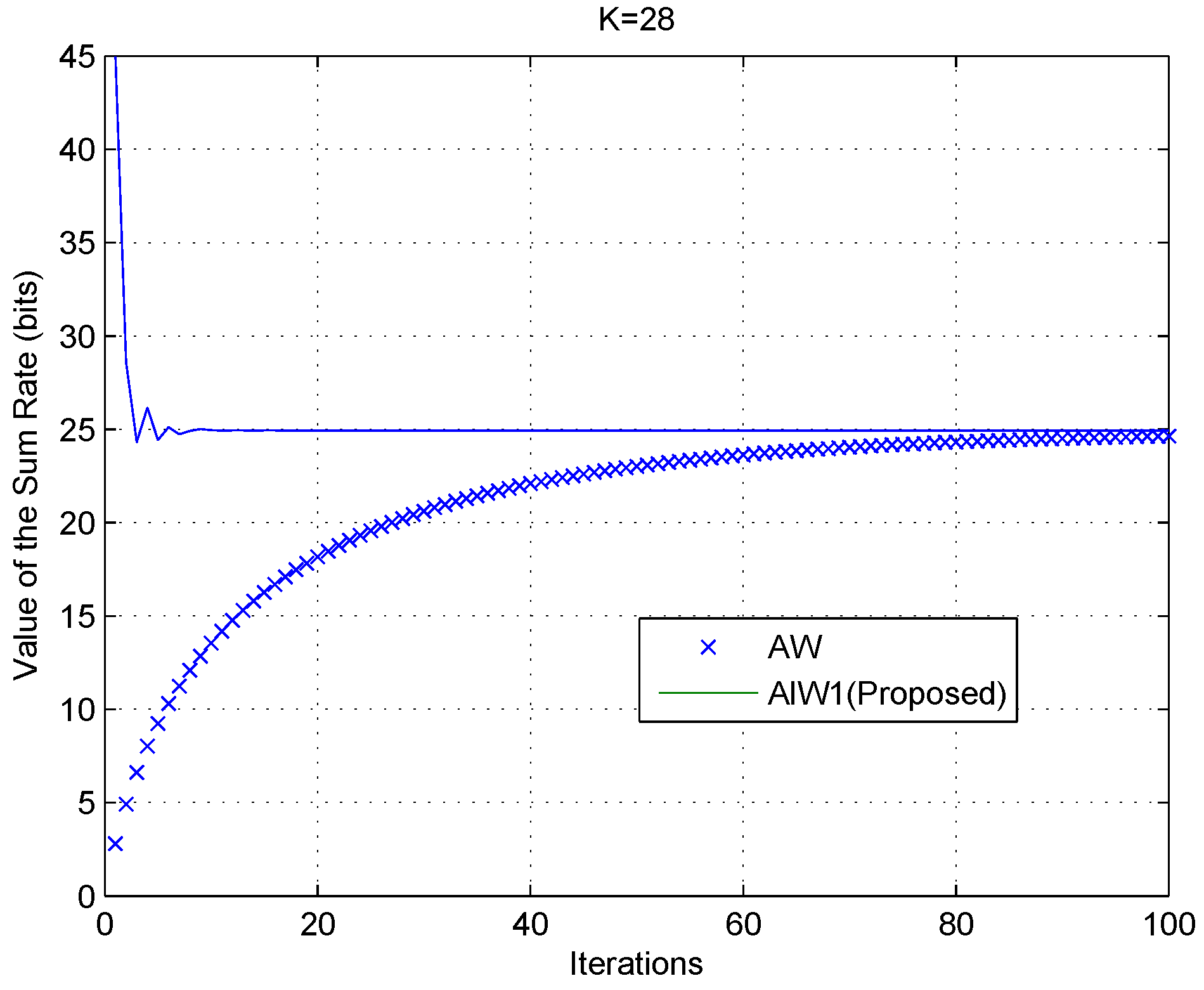
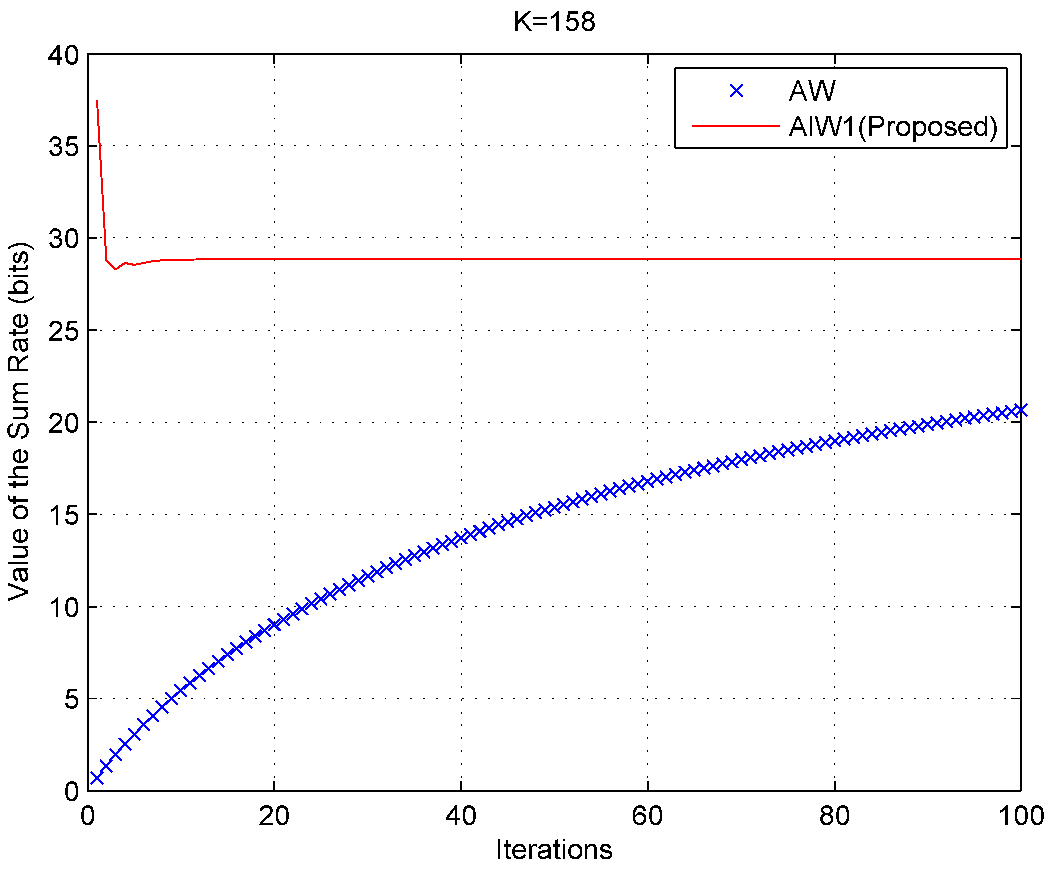
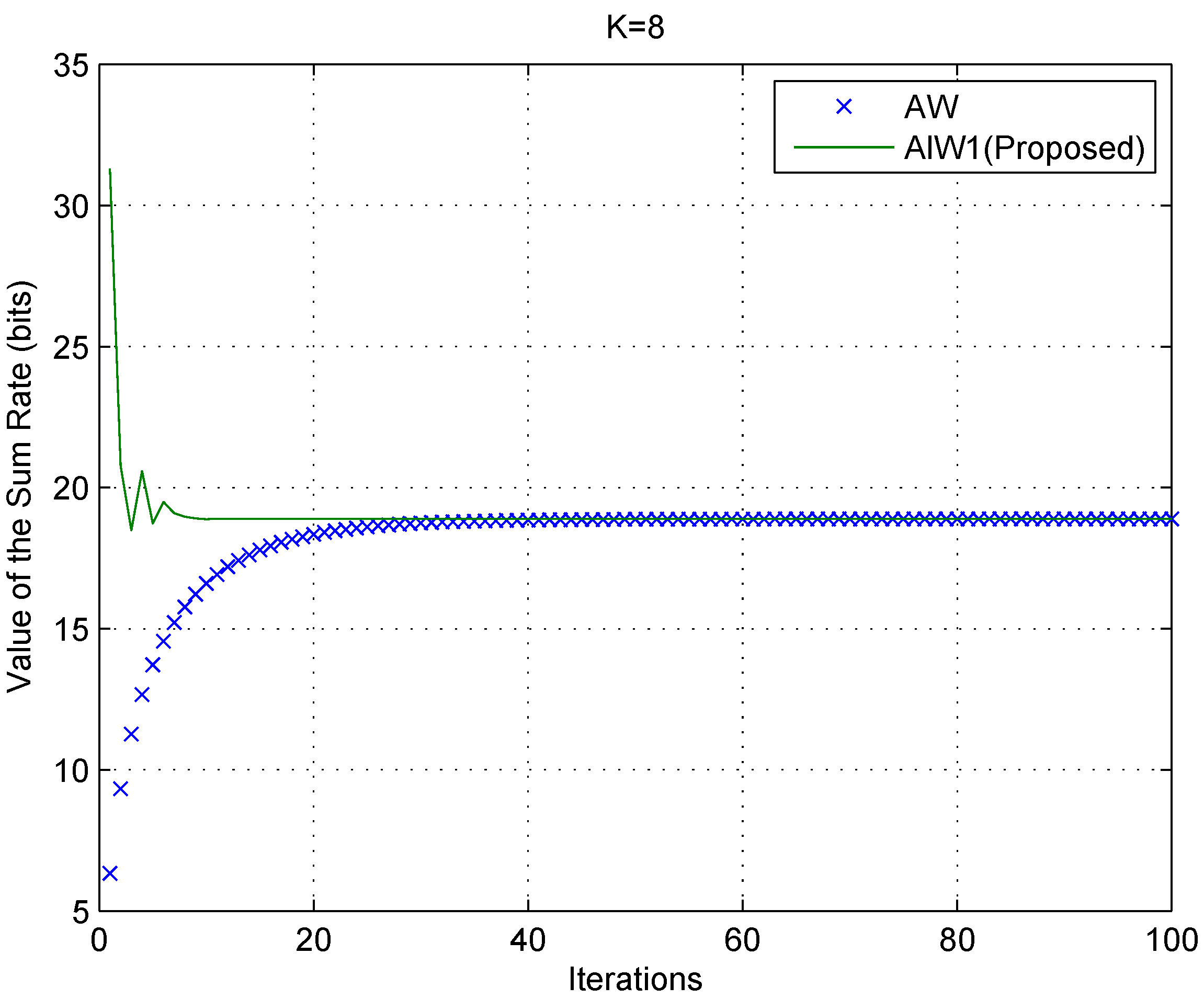
Example 2. The performance of Algorithm ALW1, compared with Algorithm AW is presented in Figure 4, Figure 5, Figure 6, Figure 7, Figure 8 and Figure 9 for different numbers of users, K, where .
Random data are generated for the channel gain vectors and the number of PUs. The numbers, denoted by K, of SUs are eight up to 158, respectively, and the number of PUs is 258. The sum-power constraints with the gains are , and the peak constraints are chosen at random.
Figure 4.
Algorithm ALW1compared with Algorithm AW, as K = 8.
Figure 4.
Algorithm ALW1compared with Algorithm AW, as K = 8.
Figure 5.
Algorithm ALW1 compared with Algorithm AW, as K = 18.
Figure 5.
Algorithm ALW1 compared with Algorithm AW, as K = 18.
Figure 6.
Algorithm ALW1 compared with Algorithm AW, as K = 28.
Figure 6.
Algorithm ALW1 compared with Algorithm AW, as K = 28.
Figure 7.
Algorithm ALW1 compared with Algorithm AW, as K = 38.
Figure 7.
Algorithm ALW1 compared with Algorithm AW, as K = 38.
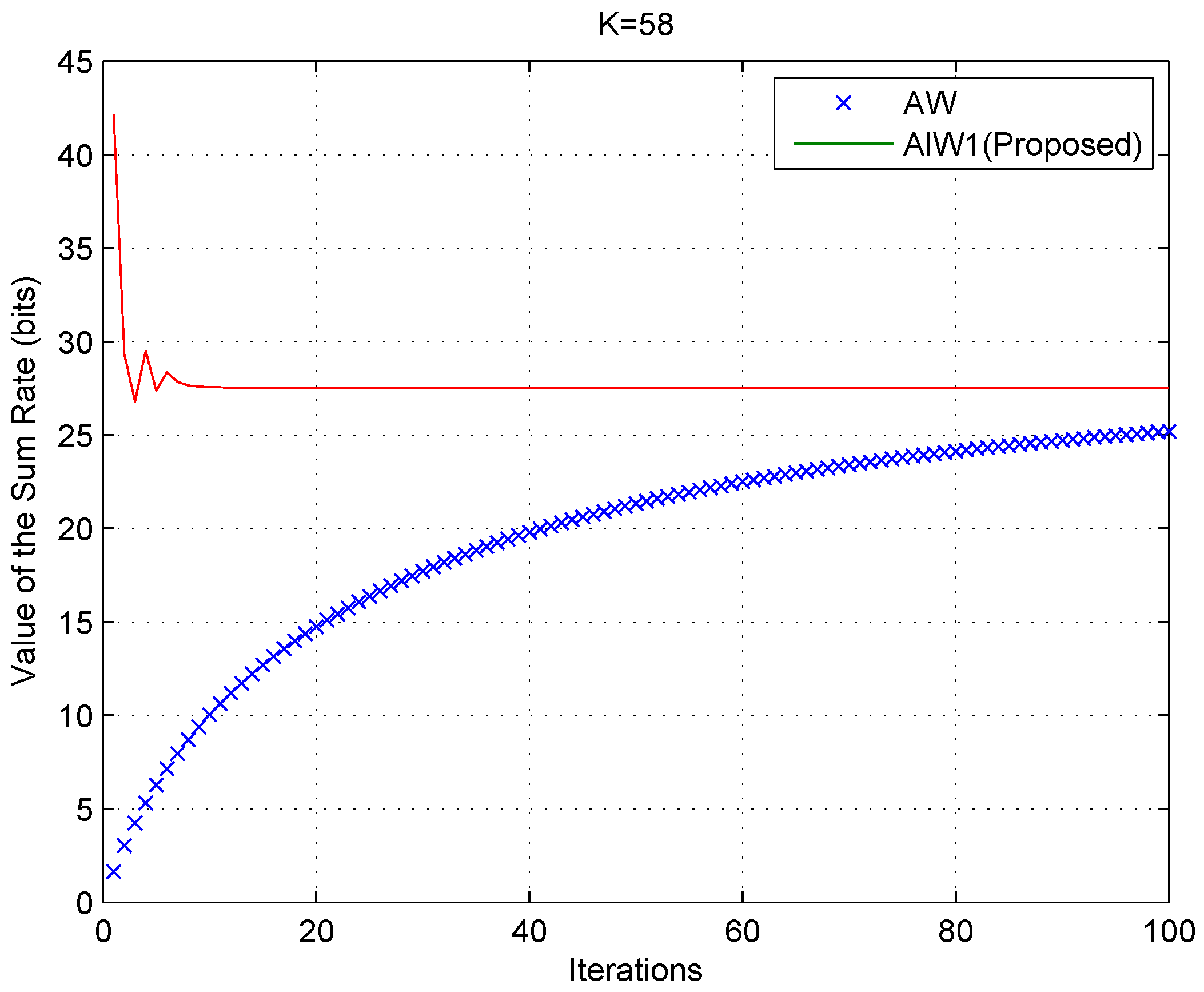
Figure 8.
Algorithm ALW1 compared with Algorithm AW, as K = 58.
Figure 8.
Algorithm ALW1 compared with Algorithm AW, as K = 58.
Figure 9.
Algorithm ALW1 compared with Algorithm AW, as K =158.
Figure 9.
Algorithm ALW1 compared with Algorithm AW, as K =158.
For
Figure 4,
Figure 5,
Figure 6,
Figure 7,
Figure 8 and
Figure 9, the solid curves and the cross markers represent the results of our proposed algorithm ALW1 and the algorithm AW, respectively. These results show that our proposed algorithm ALW1 exhibits faster convergence, even when the number of SUs is large. On the other hand, not only does ALW1 guarantee efficient convergence, but it also has a lower computational complexity. Each iteration of ALW1 scales linearly with
K; the computation complexity [
19] of the inner loop is at most
, where
c denotes the number of the inner loop iterations and
ϵ1 denotes the error tolerance for computing
Sk. The outer loop undergoes
iterations to satisfy the error tolerance
ϵ2. Compared with the complexity
of the interior point algorithm, the complexity of ALW1 is significantly reduced.


