A Multifaceted Exploration of Atmospheric Turbulence and Its Impact on Optical Systems: Structure Constant Profiles and Astronomical Seeing

Abstract

This study emphasizes the importance of conducting a comprehensive analysis considering the $C_n^2$ atmospheric parameter for a reliable assessment of the seeing value. It highlights the use of the ECMWF ERA5 model to simulate pressure, temperature, and humidity profiles, enabling the evaluation of optical degradation. Accurate modeling and monitoring of temperature and humidity variables are emphasized for precise data in optical communication and astronomical observations. It also discusses the significance of optical turbulence models in understanding the impact of atmospheric turbulence on optical system performance. The validation of the selected $C_n^2$ models is thoroughly analyzed. To evaluate the impact of the boundary layer on seeing conditions, three factors are considered. First, ERA5 data is used to simulate surface $C_n^2$ values using the PAMELA model. Second, typical $C_n^2$ values for specific dates in Redu are obtained. Finally, the thickness of the boundary layer, denoted as h_bl, is calculated. This finding highlights the significant influence of the boundary layer on atmospheric seeing conditions and by incorporating I_bl into the models, a more accurate representation of the effects of the boundary layer on seeing quality is achieved.

1. Introduction

The atmosphere unfolds as an unpredictable medium marked by ever-changing refractive index fluctuations, constituting what is known as atmospheric optical turbulence. This inherent randomness arises from dynamic variations in temperature, wind velocity, and pressure, influencing the path of light as it traverses the atmosphere. The probabilistic nature of optical turbulence necessitates advanced tools—such as structure functions and the atmospheric structure parameter, denoted as $C_n^2$—for meticulous characterization. The precise measurement and classification of optical turbulence hold pivotal roles across diverse scenarios, ranging from the observation of celestial bodies with telescopes to the facilitation of optical communication in free space. The theoretical foundations and statistical underpinnings of turbulence theory owe their origins to Kolmogorov, Obukhov, and Corrsin [1,2,3], while its extension to wave propagation in random media was advanced by Fried, Tatarski, and Ishimaru [4,5,6]. Kolmogorov’s classification of turbulent eddies based on an outer scale, L₀, and an inner scale, l₀, laid the groundwork for understanding turbulence dynamics.

The significance of optical turbulence is quantified by the refractive index structure constant, $C_n^2$ [7]. This parameter exhibits variability based on geographical location, altitude, and time of day. In addition to the factors mentioned, it is essential to acknowledge the role of aerosol scattering in contributing to optical turbulence. Aerosol scattering introduces an additional layer of complexity, particularly at higher elevations, and is sometimes referred to as the adjacency effect in remote sensing. While our study focuses primarily on turbulence-induced atmospheric blur, the influence of aerosol scattering on optical observations is a relevant consideration. Although we do not delve into the details of aerosol scattering in this work, its significance adds another dimension to the understanding of atmospheric effects on optical observations. Diverse temperature distribution characteristics in different locations manifest in distinct $C_n^2$ values. At lower altitudes beneath the tropopause, where the most substantial temperature gradients exist, $C_n^2$ values are larger due to higher atmospheric pressure and air density. As altitude increases, atmospheric pressure and air density decrease, leading to diminished $C_n^2$ values until the tropopause, where strong wind shear introduces further variations. $C_n^2$ values for intense turbulence can reach up to 10⁻¹³ m^−2/3, while weaker conditions near the ground can decrease to 10⁻¹⁷ m^−2/3. The altitude-dependent behavior of $C_n^2$ is categorized into three layers: the surface layer, influenced by wind interactions and covering a few tens of meters; the planetary boundary layer (PBL), affected by earth–atmosphere interactions with varying thickness and height contingent on temperature and surface topography; and the free atmosphere, situated above the boundary layer, influenced by wind shear and gravity waves, extending approximately 10–12 km. This intricate interplay of factors underscores the complexity and importance of optical turbulence, forming the core motivation for its thorough exploration and understanding in various scientific applications.

The subsequent sections of this paper are organized as follows: Section 2 delves into an exploration of four optical turbulence models that predict refractive index profiles, denoted as $C_n^2$ based on meteorological data. Section 3 provides a comprehensive overview of common figures employed in astronomy to illustrate the impact of atmospheric turbulence on telescope performance along with their validation. Section 4 constitutes the crux of this paper, elucidating the simulation process involving pressure, temperature, humidity, and hourly $C_n^2$ profiles using the European Centre for Medium-Range Weather Forecasts (ECMWF) model in Redu, Belgium. The primary objective is to assess and validate the seeing value in February 2019, leveraging ECMWF (ERA5) and all models for Redu. The term seeing pertains to the capacity for gauging atmospheric turbulence. In essence, ground-based telescopes encounter limitations in their observational acuity due to the presence of atmospheric turbulence, commonly denoted as “seeing”. To enhance the precision of the seeing value computation, the contribution of the boundary layer height is integrated into the preceding $C_n^2$ simulations. In the context of this paper, the term “boundary layer” is employed to denote the understanding of turbulence and structural constants within this layer.

2. Finite-Dimensional (Parametric) Model

This model involves certain parameters aimed at enhancing specific meteorological parameters and mirroring the intricacies found in real observations of $C_n^2$. The model’s entirety is encapsulated within its parameters, rendering it a parametric model. In contrast to non-parametric models that exclusively utilize altitude to portray the changes in $C_n^2$, parametric models incorporate additional variables for this representation.

The primary models utilized in this research are Marzano, Trinquet–Vernin (TV), and the Dewan model based on the Air Force Geophysics Laboratory (AFGL) radiosonde. However, the parameter $C_n^2$ can solely be characterized by the Pamela model within the boundary layer. For a more in-depth exploration of additional $C_n^2$ models, please refer to the conclusion section.

2.1. AFGL (Dewan)

Models from the Air Force Geophysics Laboratory (AFGL) [7], derived from thermosonde data, are limited in their applicability to the upper atmosphere, offering detailed profiles. Utilizing Tatarski’s concept [8], this turbulence model designed for the upper atmosphere is extended to optical turbulence, specifically defined by the refractive index structure parameter denoted as $C_n^2$. Dewan relies on the connection between the outer scale and the statistical variation in wind shear and is valid only above the boundary layer. This model transforms radiosonde information into profiles of $C_n^2$, employing the subsequent equation:

$$C_n^2 = a^{2}a {L_0 }^{4/3} M{ }^2 \left(h\right)$$

(1)

where [9,10]

$$M=\left(\frac{-79 \times {10}^{-6 }P}{T^2}\right)\left(1+\frac{\mathrm{15,500}q}{T}\right)\left(\frac{ dT}{ dh}+\gamma - \frac{7800}{1+\frac{\mathrm{15,500}q}{T}} . \frac{dq}{dh}\right)$$

(2)

within this formula, the variables P and T correspond to pressure in millibars and temperature in kelvin respectively. γ and h denote the adiabatic lapse rate, equating to 9.8 × 10 ⁻³ km⁻¹ (indicating that as an ascending air parcel rises by 100 m, it cools by approximately 0.98 degrees) [8,9] and height in meters, respectively. Additionally, q signifies the specific humidity. Typically, for optical ranges in which humidity is unimportant, q assumes a value of 0, rendering M (mean refractive index gradient or vertical gradient of potential refractive index) interchangeable with (3). In the lower layer, γ can be disregarded [5] given that temperature gradients surpass γ substantially. According to Tatarski [8], L₀ denotes the outer scale or mixing length. In (1), the value of a²a was established through experimentation, and Gurvich [10] determined a global factor of 2.8 [11] for this value, a finding subsequently adopted by other researchers.

$$M=\left(\frac{-79 \times {10}^{-6 }P}{T^2}\right)+\left(\frac{dT}{dh}+\gamma \right)$$

(3)

For both the troposphere and the stratosphere, the equation formulated to calculate L₀ takes the following form [7,8]:

$$L_0^{4/3}={ \left(0.10\right)}^{4/3}\times {10}^Y$$

(4)

the value of Y is dependent on the vertical positioning of the tropopause:

$$Y\left\{\begin{array}{c}1.64+42.0 S\\ 0.506+50.0 S\end{array}\right.$$

(5)

Additionally, in conjunction with a linear regression connecting the outer scale and wind shear:

$$L_0^{4/3}\left\{\begin{array}{c}{0.1}^{4/3}{10}^{1.64+42.0 S}\hspace{1em}\hspace{1em} \mathrm{T}\mathrm{r}\mathrm{o}\mathrm{p}\mathrm{o}\mathrm{s}\mathrm{p}\mathrm{h}\mathrm{e}\mathrm{r}\mathrm{e}\\ {0.1}^{4/3}{10}^{0.506+50.0 S}\hspace{1em}\hspace{1em} \mathrm{S}\mathrm{t}\mathrm{r}\mathrm{a}\mathrm{t}\mathrm{o}\mathrm{s}\mathrm{p}\mathrm{h}\mathrm{e}\mathrm{r}\mathrm{e}\end{array}\right.$$

(6)

where the wind shear, denoted as S, is defined in the subsequent manner, and L₀ is represented in meters:

$$S={\left.\left[{\left(\frac{du}{dh}\right)}^2+{\left(\frac{dv}{dh}\right)}^2\right.\right]}^{ \frac{1}{2}}$$

(7)

In (7), the variables u and v stand for the north and east winds, respectively.

Ultimately, a conclusive refractive index structure parameter, $C_n^2$, profile has been established from:

$$C_n^2=2.8 L_0^{4/3}{{\left.\left[\left(\frac{-79 \times {10}^{-6}P}{T^2}\right)+\left( \frac{dT}{dh}+\gamma \right)\right.\right]}^2 }^{ }$$

(8)

2.2. Marzano

The refractive index structure constant is described by the equation presented in (1), formulated by Tatarski. If we consider the modified variant of M proposed by Masciadri for optical scenarios [12,13,14,15,16], it can be expressed as follows:

$$M=\left(\frac{-79\times {10}^{-6 }P}{T^{ }\theta }\right)+\frac{d\theta }{dh}$$

(9)

$\theta$ is potential temperature ($\theta =T({\frac{1000}{P})}^{\raisebox{1ex}{$2$}\!\left/ \!\raisebox{-1ex}{$7$}\right.}$), T is the temperature in kelvin, and P is the pressure in mbars).

As the buoyancy is directly connected to the potential temperature, consequently, M transforms to:

$$M=\zeta B$$

(10)

where

$$\mathsf{\xi }\triangleq -79\frac{P}{g_{0}T} {\times 10}^{-6}$$

(11)

$g_0$ represents gravitational acceleration. The turbulence layers can be identified using the gradient Richardson number Ri.

$$Ri\triangleq \frac{B}{S^2}$$

(12)

where the vertical shear of the horizontal wind speed components is denoted by the random variable S [s⁻¹] as it is mentioned in (7). A high degree of turbulence is indicated by a diminished Ri value. The threshold is defined as Ri ≤ Ri_c, where the critical Richardson number Ri_c is typically around 0.25, a value substantiated by empirical evidence. Moreover, the outer turbulence scale L₀, which is often not precisely known, is treated as a stochastic variable. Consequently, we aim to calculate the anticipated value of $C_n^2$ using the subsequent equation.

$$〈C_n^2〉=2.8{\int }_{L_{0,m}}^{L_{0,M}}{L}_0^{\raisebox{1ex}{$4$}\!\left/ \!\raisebox{-1ex}{$3$}\right.}{\int }_{\frac{B}{{Ri}_c}}^{+\infty }{\int }_{\frac{B}{S^2}\le {Ri}_c}^{+\infty }{\int }_{-\infty }^{+\infty }{M}^2{p}_{C_n^2}\left(L_0,S,B,Q\right)\mathit{dQdBdSd}{L}_0$$

(13)

in (13), Q represents the gradient of specific humidity (a parameter of minimal significance in the optical domain), and the probability density function, denoted as $p_{C_n^2}$, is deduced from well-established measurements. The intricate nature of this integral makes its direct computation challenging. To address this complexity, Marzano introduced simplifications to enhance its practicality. Specifically, he adopted the simplifications introduced by Van Zandt [7], presuming the independence of various parameters’ influences.

$$p_{C_n^2}\left(L_0,S,B\right)=p_{L_0}\left(L_0\right) p_S\left(S\right) p_{B,Q}\left(B,Q\right)$$

(14)

$$p_{L_0}\left(L_0\right)=\frac{1}{L_{0,M} -L_{0,m}}u\left(L_{0,m}\le L_0\le L_{0,M}\right)$$

(15)

$${ p}_S\left(S\right)=p_S\left(L_{0,\mathit{eff}},S\right)$$

(16)

In the scenario where L₀ is assumed to follow a uniform distribution, the determination of the lower limit $L_{0,m}$ and upper limit $L_{0,M}$ is guided by empirical investigations [13]. These ranges typically span from 0.1 to 5 m and 30 to 100 m [12], or alternatively from 3 to 100 m [16]. Accordingly, this selection results in the subsequent formulation for the probability density function $p_S$,

$$p_S\left(L_0,S\right)=\frac{S}{{\sigma }_S^2\left(L_{0,\mathit{eff}}\right)}\mathit{exp}\left(-\frac{S^2+{〈S〉}^2}{2{\sigma }_S^2\left(L_{0,\mathit{eff}}\right)}\right)I_0\left(\frac{S〈S〉}{{\sigma }_S^2\left(L_{0,\mathit{eff}}\right)}\right)$$

(17)

the symbol I₀ denotes the modified Bessel function of the first kind, featuring variances ${\sigma }_S^{}$ and $L_{0,\mathit{eff}}$. The term Rice–Nakagami distribution is attributed to this statistical distribution due to its initial derivation from the Nakagami approach. In situations where the expectation value 〈S〉 is zero, the distribution transforms into the Rayleigh distribution, as documented in the literature [13].

$${\sigma }_S^{}\left(L_0\right)={\sigma }_{S,0}{L}_0^{{\alpha }_{L_0}}{ \left|〈B〉\right|}^{{\alpha }_B}{ 〈\rho 〉}^{{\alpha }_{\rho }}$$

(18)

by employing coefficients that have been established through empirical examination—namely ${\sigma }_{S,0}$ = 0.18, ${\alpha }_{L_0}$ = −0.3, ${\alpha }_B$ = 0.25, and ${\alpha }_{\rho }$ = −0.15, with $\rho$ representing density—the following transformations are implemented.

$$L_{0,\mathit{eff}} \triangleq {〈{L_0}^{\frac{4}{3}}〉}^{\frac{3}{4}}={\left[\frac{1}{L_{0,m}-L_{0,M}}{\int }_{L_{0,M}}^{L_{0,m}}{L}_0^{\raisebox{1ex}{$4$}\!\left/ \!\raisebox{-1ex}{$3$}\right.}d{L}_0\right]}^{ \frac{3}{4}}={\left[\frac{3}{7}\frac{L_{0,M}^{\frac{7}{3}} -L_{0,m}^{\frac{7}{3}}}{L_{0,M} -L_{0,m}}\right]}^{\frac{3}{4}}$$

(19)

Given that the hypothesis involves a correlation coefficient of ±1 between B and Q, there is no need to explicitly define $p_{B,Q}(B,Q)$ or to formulate (14). Thus, we can reformulate (13) as follows:

$$〈C_n^2〉=2.8\left({〈M〉}^2+{\sigma }_M^2\right) L_{0,\mathit{eff}}^{\frac{4}{3}}{F}_S$$

(20)

$$F_S \triangleq {\int }_{\sqrt{\raisebox{1ex}{$\left|〈B〉\right|$}\!\left/ \!\raisebox{-1ex}{${Ri}_c$}\right.}}^{+\infty }{p}_S\left(L_{0,\mathit{eff}},S\right)dS=Q_1\left(\frac{〈S〉}{{\sigma }_S\left(L_{0,\mathit{eff}}\right)},\frac{\sqrt{\left|〈B〉\right|/{Ri}_c}}{{\sigma }_S\left(L_{0,\mathit{eff}}\right)}\right)$$

(21)

$Q_1$, denoted as the initial Marcum function, serves as a representation of the probability that the observed layer exhibits turbulence or the proportion of it that is anticipated to contribute to the mean value of $〈C_n^2〉$. In the optical context, in which ${\sigma }_M^2$ is equivalent to ${\left({\sigma }_B\right)}^2$ and ${\sigma }_M^2$ is significantly smaller than ${〈M〉}^2$, (20) is consequently simplified to:

$$〈C_n^2〉\cong 2.8{〈M〉}^2{L}_{0,\mathit{eff}}^{\frac{4}{3}}{F}_S$$

(22)

Equation (22) illustrates the similarity between the expression for $C_n^2$ and the Tatarski formula presented in (1). The model developed by Marzano is only applicable above the boundary layer.

2.3. Trinquet–Vernin (TV)

Differing from the methodology proposed by Tatarski, the framework introduced by this model [17] for inferring $C_n^2$ from the temperature structure constant $C_T^2$ demonstrates a lack of dependence on temperature. The Gladstone equation [18] establishes a relationship between these two quantities, thereby characterizing their interdependence.

$$C_n^2={\left(\frac{-80\times {10}^{-6}P}{T^2}\right)}^2{C}_T^2$$

(23)

herein, P denotes the atmospheric pressure measured in hPa, while T represents the absolute temperature.

Through the application of statistical analysis, it is established that the magnitude of $C_T^2$ exhibits a direct proportionality to the alignment of the potential temperature gradient and the wind shear S(h):

$$C_T^2 (h)=\varphi (h)(\frac{d\theta }{dh}){S\left(h\right)}^{\frac{1}{2}}$$

(24)

in this context, the function ϕ(h) constitutes an empirical parameter that has been determined through the analysis of 160 meteorological balloons across 8 distinct locations during the chosen flights [18]. The profiles corresponding to the free atmosphere and the boundary layer are provided in

Table 1. The vertical distribution of ϕ(h) at different altitudes.

Altitude (m)	Boundary Layer $\mathit{\varphi }\left(\mathit{h}\right)$	Altitude (m)	Free Atmosphere $\mathit{\varphi }\left(\mathit{h}\right)$
5	2.8349920	1500	0.2202239
55	0.7825773	2500	0.1232994
105	0.2851246	3500	0.1220847
155	0.2247893	4500	0.1116992
205	0.2339369	5500	7.9565063 × 10−2
255	0.2368697	6500	7.6611020 × 10−2
305	0.1393718	7500	9.4689481 × 10−2
355	0.1697904	8500	8.2437001 × 10−2
405	0.1350916	9500	8.5563779 × 10−2
455	0.1151705	10,500	7.9648279 × 10−2
505	0.1201656	11,500	5.9562359 × 10−2
555	0.1242000	12,500	4.4496831 × 10−2
605	0.1528365	13,500	4.5322943 × 10−2
655	0.1258108	14,500	3.8577948 × 10−2
705	0.1038473	15,500	4.9237989 × 10−2
755	9.6003376 × 10−2	16,500	4.5535788 × 10−2
805	8.3205506 × 10−2	17,500	4.5892496 × 10−2
855	0.1061958	18,500	3.9653547 × 10−2
905	9.4715632 × 10−2	19,500	4.1269500 × 10−2
955	0.1022552

. In contrast to the Tatarski-equation-derived model, the $C_n^2$ value in this context demonstrates proportionality to $\left(\frac{d\theta }{ dh}\right)$ as opposed to being proportional to ${\left(\frac{d\theta }{ dh}\right)}^2$.

2.4. Pamela

Regarding surface-boundary-layer $C_n^2$ magnitudes, the PAMELA model [19,20,21] stands as one of the most sophisticated models, covering a significant range of altitudes, extending to several hundreds of meters. Apart from acquiring a solitary measurement (or estimation) of air temperature, pressure, and wind speed at the intended $C_n^2$ evaluation level, this model demands an extensive array of input parameters. It offers compelling insight into the effective delineation of the boundary layer, a pivotal aspect often lacking in numerous parametric models.

In this segment, the initial step involves the computation of the refractive index structure parameter, denoted as $C_n^2:$

$$C_n^2=\frac{\left(b{K}_h\right)}{{\epsilon }^{1/3}}\frac{dn}{dh}$$

(25)

herein, b represents a constant frequently estimated around 2.8, while $K_h$ denotes the heat turbulent exchange coefficient. ε pertains to the rate of eddy dissipation, and the gradient of the refractive index $\frac{dn}{dh}$ stands as follows:

$$\frac{dn}{ dh}=\frac{(-77.6 \times {10}^{-6}Pa)T*{\varphi }_h(\frac{ h}{ L} )}{K_{v}h{T}^2}$$

(26)

where k_v represents von Karman’s constant with a value of 0.4, Pa signifies the atmospheric pressure in millibars, T denotes the atmospheric temperature in kelvin, h corresponds to the height in meters, and L stands for the Monin–Obukhov length along with the dimensional temperature gradient. Furthermore, ${\varphi }_h$ and ${\varphi }_M$ are characterized as:

$${\varphi }_h=\left\{ \begin{array}{c}{\varphi }_h\left(\frac{ h}{ L}\right)=0.74+4.7\left(\frac{ h}{ L}\right), p>0, \\ {\varphi }_h\left(\frac{ h}{ L} \right)=0.74{\left.\left[1 - 9\left(\frac{ h}{ L}\right)\right.\right]}^{-0.5}, p\le 0,\end{array}\right.$$

(27)

$${\varphi }_m=\left\{ \begin{array}{c}{ \varphi }_m\left(\frac{ h}{ L}\right)=1+5 \left(\frac{ h}{ L}\right), p>0, \\ {\varphi }_m\left(\frac{ h}{ L}\right)={\left.\left[1 - 16\left(\frac{ h}{ L}\right)\right.\right]}^{-\frac{1}{4}}, p\le 0,\end{array}\right.$$

(28)

The subsequent equation is employed for the computation of the characteristic temperature T^∗:

$$T*=\frac{-H}{c_P\rho u\mathit{\star }}$$

(29)

here, ρ signifies the atmospheric density in kilograms per cubic meter, attainable via ρ = Pa/(2.9T). The specific heat under constant pressure, denoted as $c_p$ and equal to 1004 J/(kg·K), as well as H, the sensible heat flux, are involved in the calculation. In accordance with the subsequent formula, the friction velocity u⋆ is defined as:

$$u\mathit{\star }=\frac{k_v\overline{v_0}}{ln (\frac{h}{ h_r})-{\psi }_m}$$

(30)

in (30), ${\overline{v}}_0$ signifies the average wind speed, $h_r$ corresponds to the length of the surface roughness, proportionate to the average height of the Earth’s surface in centimeters for typical urban and rural conditions as outlined in

Table 2. Length of the surface roughness.

Surface Type	Roughness Length (cm)
Village	40
Town	55
Light-density residential	108
Park	127
Office	175
Central business district	321
Heavy density residential	370
Grass (5–6 cm)	0.75
Alfalfa	2.7
Long grass	3
Grass (60–70 cm)	11.4
Open brush or scrub	16
Wheat	22
Dense brush or scrub	25
Forest clearing or cutovers	32–48
Corn	74
Coniferous forest	110
Citrus orchard	198
Fir forest	283

and in (31). Furthermore, the diabatic influence function for momentum, ${\psi }_m$, is derived from:

$$h_r\cong \mathit{Exp} [-2.85+1.2\mathit{ln}\left(h_f\right)] {,h}_f<700 \mathrm{cm}$$

(31)

$${\psi }_m=\left\{\begin{array}{ll}-5\left(\frac{ h}{ L}\right),& P>0,\\ \mathit{ln}\left[\left( \frac{1+y^2}{2}\right){\left( \frac{1+y^{ }}{2}\right)}^2\right]- 2\mathit{arctan}\left(y\right)+\frac{\pi }{2}, y={\left[1-16\left(\frac{h}{L}\right)\right]}^{ \frac{1}{4}},& P\le 0\end{array}\right.$$

(32)

To determine the heat turbulent exchange coefficient $K_h$, the knowledge of the friction velocity u* is necessary. The expression for $K_h$ is given by:

$$K_h=\frac{K_{v }u*h}{{\varphi }_h(\frac{ h}{ L})}$$

(33)

Moving forward, the discussion will focus on the two remaining parameters: ε, which represents the rate of eddy dissipation, and L, denoting the Monin–Obukhov length. Under steady-state conditions, in accordance with the Kolmogorov hypothesis of universal equilibrium [8], ε = M + B. Wind shear generates energy represented by M, while buoyancy generates energy denoted as B. The energy generation rate attributed to wind shear is defined as

$${M=k}_m{\left|\frac{d\overline{v}}{dh}\right|}^2$$

(34)

the turbulent momentum exchange coefficient, $k_m$, and the average wind speed,$\overline{v}$, at reference height h are involved in the equation. The energy generation rate resulting from buoyancy can be computed utilizing the following expression.

$$B={-k_h}_{}\frac{g_0}{\theta }\frac{d\theta }{dh}$$

(35)

considering the standard gravitational acceleration of the Earth’s surface, denoted as $g_0$ = 9.8065 m/s², along with the average potential temperature θ in kelvin and the term $k_h$ in (33).

Another crucial parameter for determining the gradient of the refractive index, as outlined in (26), is the Monin–Obukhov length (L) [22],

$$L={\left[\left(0.00435P+0.0037P^3\right)h_r^{ -{\left[0.5-0.23\left|P\right|+0.0325P^2\right]}^{ }}\right]}^{-1}$$

(36)

as indicated in (31), h_r represents the length of surface roughness and P denotes the Pasquill stability category, which can be approximated through the following equation:

$$P=\frac{1}{2} (4 - c_w+{ c}_r)$$

(37)

the radiation class, denoted as $c_r$, and the wind speed class, indicated as $c_w$, are pertinent in the following manner and can be calculated using the subsequent formulas:

$$c_r=\left\{\begin{array}{l}\frac{R}{300}, H>0, \\ -1, H\le 0, cc\ge 4\\ -2, H\le 0, cc<4\end{array}\right.$$

(38)

here, R represents the solar irradiance incident in W/m² during the day. During nighttime, when the cloud cover exceeds 50%, the value of $c_r$ is set to −1, while it is considered to be −2 when the cloud cover is less than 50%.

Similarly, the wind speed class, denoted as $c_w$, is determined as follows:

$$c_w=\left\{\begin{array}{c}\left(\frac{{\overline{v}}_0}{2}\right), {\overline{v}}_0\le 8 \mathrm{m}/\mathrm{s}\\ 4, {\overline{v}}_0>8 \mathrm{m}/\mathrm{s}\end{array}\right.$$

(39)

3. Optical Parameters in Astronomy

Essential atmospheric parameters—such as the Fried parameter, denoted as $r_0,$ and the seeing, represented as $\mathit{\varepsilon }$, are requisite for the formulation of advanced techniques aimed at achieving high angular resolution. The aforementioned $C_n^2$ profiles can serve as instrumental resources for extracting these crucial parameters.

3.1. Fried Parameter

Turbulence significantly affects optical system performance [2,23,24,25] and is gauged by this parameter. Larger apertures improve image resolution up to the coherence length (Fried parameter), denoting maximum telescope diameter for resolution. Smaller $r_0$ values ($r_0$ < D) signal significant turbulence, warranting adaptive optics, while larger values ($r_0$ > D) indicate milder turbulence. This parameter is also defined in (40) as representing refractive index changes’ integrated impact. This parameter, as delineated in Equation (40), encapsulates the cumulative influence of refractive index variations for a plane wave following a horizontal trajectory [26]:

$$r_0={\left[0.423{\left(\frac{2\pi }{\lambda }\right)}^2 \sec z{\int }_{h_0}^{h_0+L}{C}_n^2(h)dh\right]}^{-3/5}$$

(40)

Conversely, when considering a spherical wave traversing a horizontal path:

$$r_0={\left[0.158{\left(\frac{2\pi }{\lambda }\right)}^2 \sec z{\int }_{h_0}^{h_0+L}{C}_n^2(h)dh\right]}^{-3/5}$$

(41)

here, h₀ represents the position of the receiver, while h₀ + L denotes the source location. The variable z signifies the zenith angle, and the integration encompasses the distance from the telescope to the highest point of turbulence. The Fried parameter, expressed in centimeters, assumes the role of a length unit and usually spans the range of turbulence altitudes. To provide additional details about the Gaussian beam and transverse coherence length, kindly refer to [27].

3.2. Seeing

Atmospheric turbulence disperses laser beams, degrading angular resolution. “seeing” in astrophysics gauges turbulence, impacting images and positions. Telescopes’ resolutions link to wavelength-to-coherence length ratio, which is called “astronomical seeing”. Ground-based telescopes are limited by atmospheric turbulence, “seeing” [23,28]. Equation (42) reveals larger $r_0$ boosts seeing, tied to location.

$$\varepsilon =0.98 \frac{\lambda }{r_0}$$

(42)

With refractive index parameter, seeing is expressed,

$$\varepsilon ={5.25{\lambda }^{-1/5}\left[\sec z{\int }_{h_0}^{h_0+L}{C}_n^2(h)dh\right]}^{\frac{3}{5}}$$

(43)

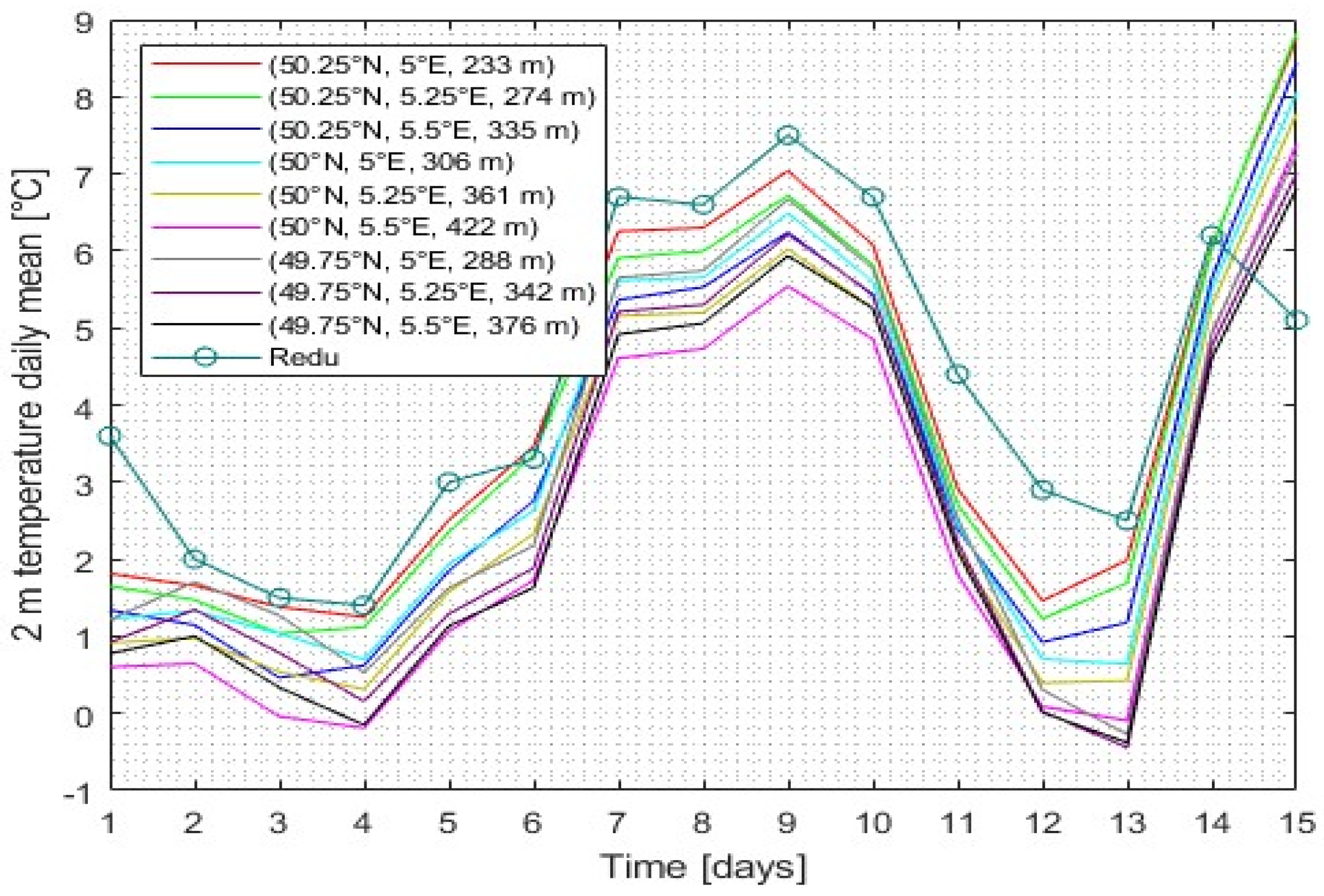
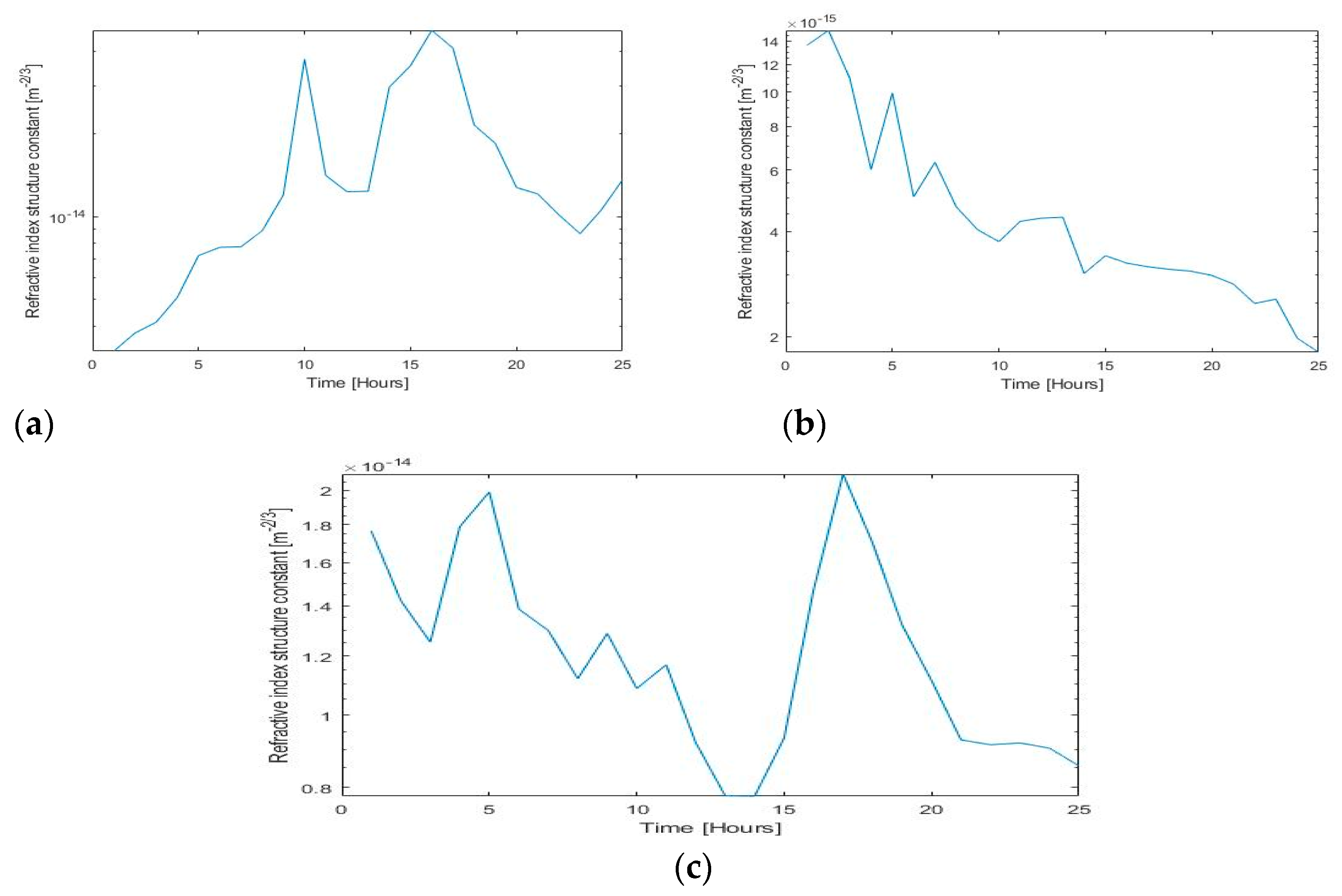
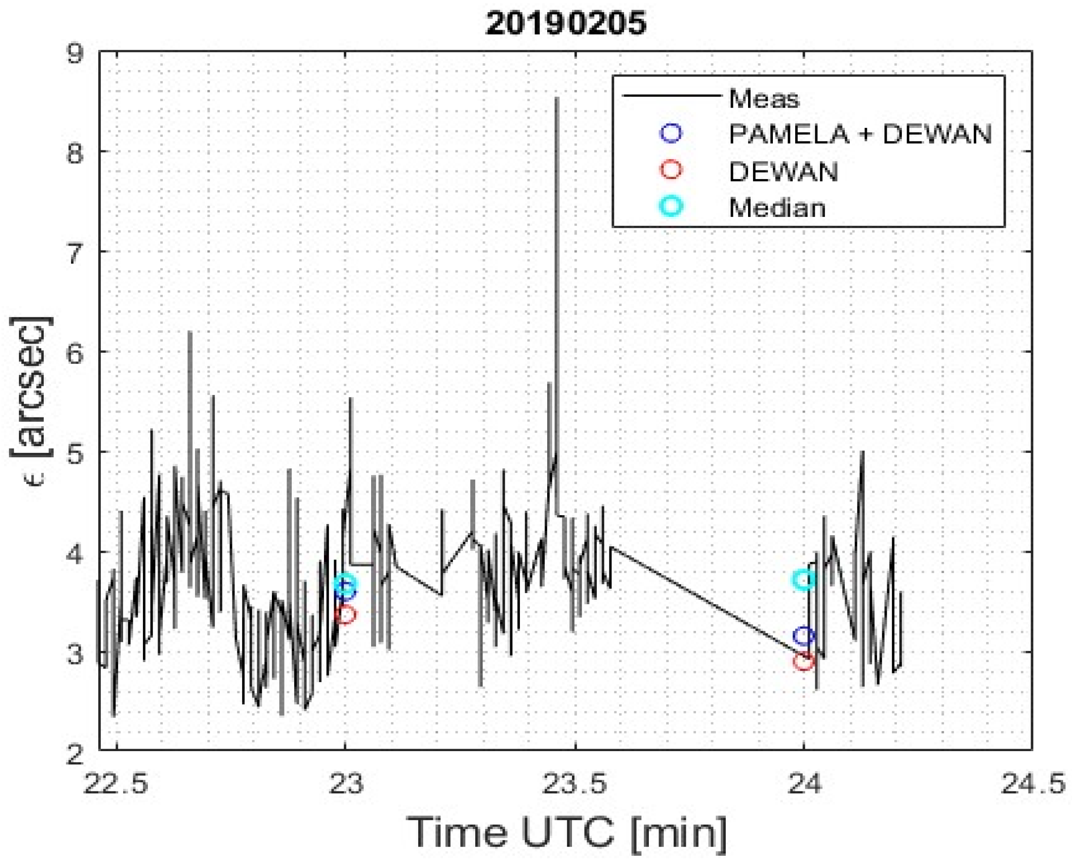
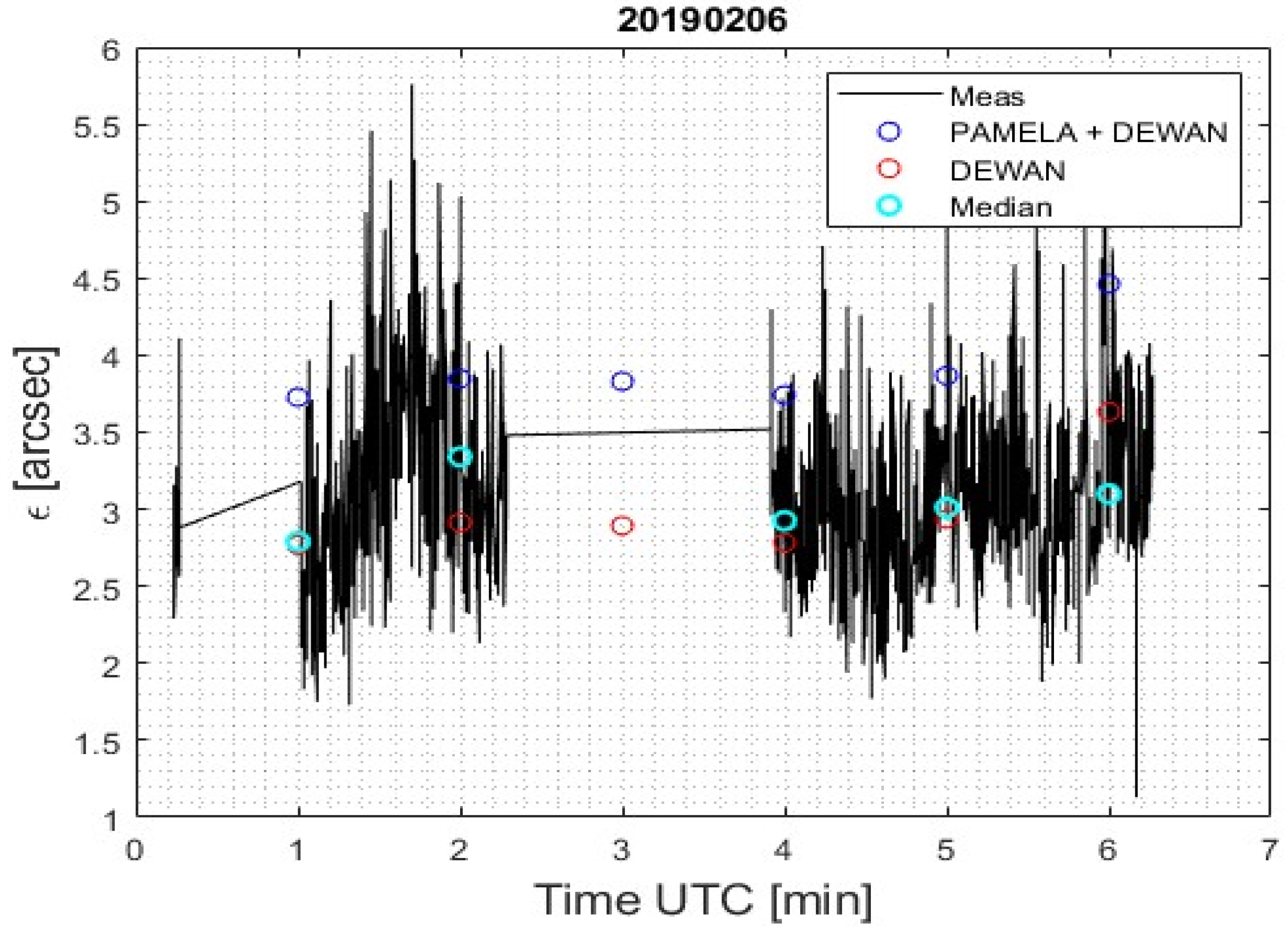
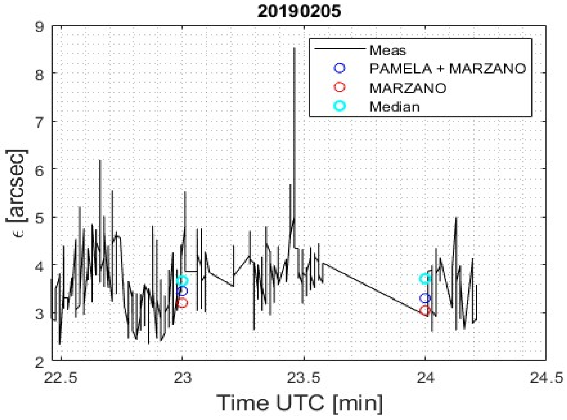
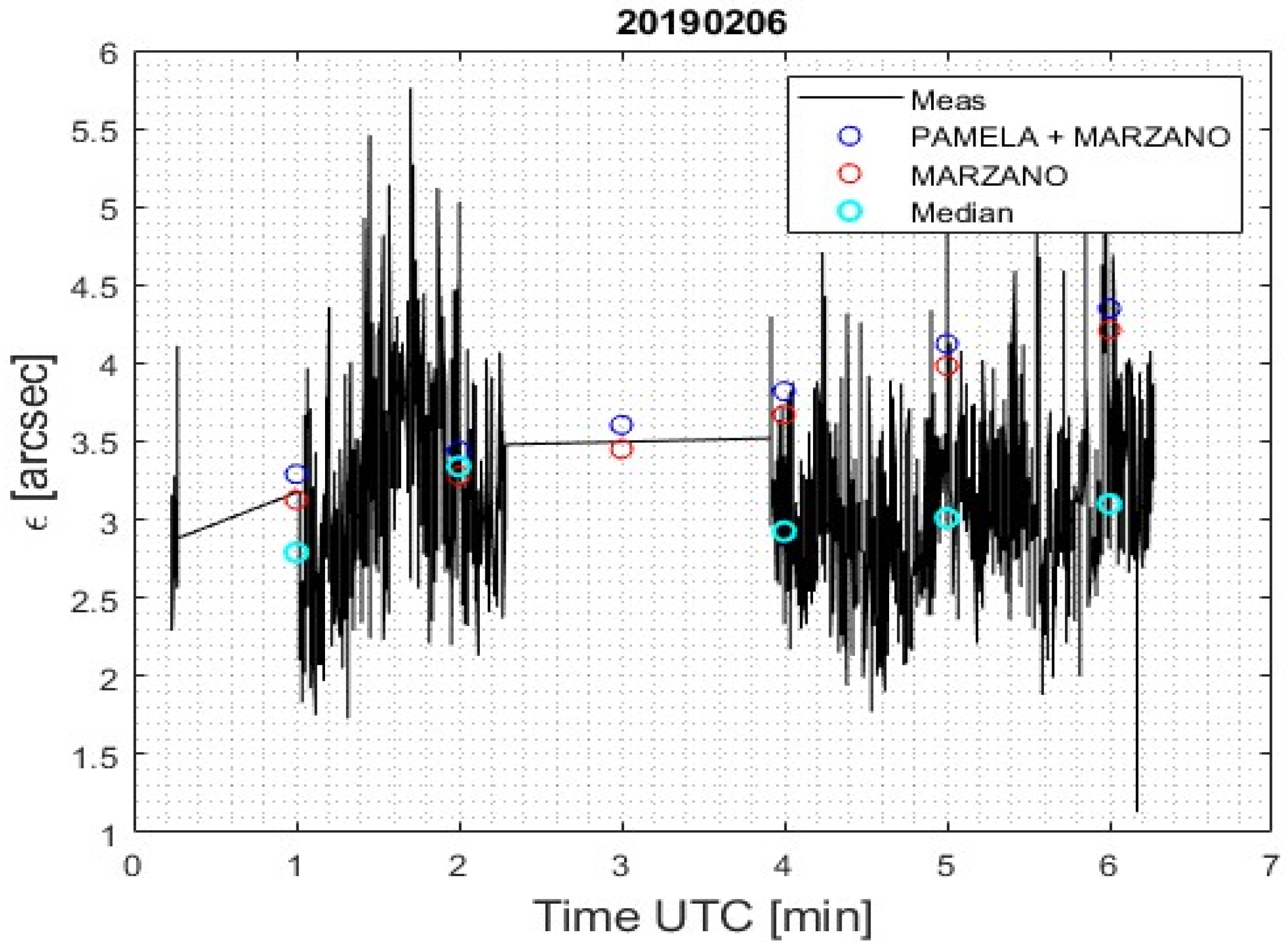
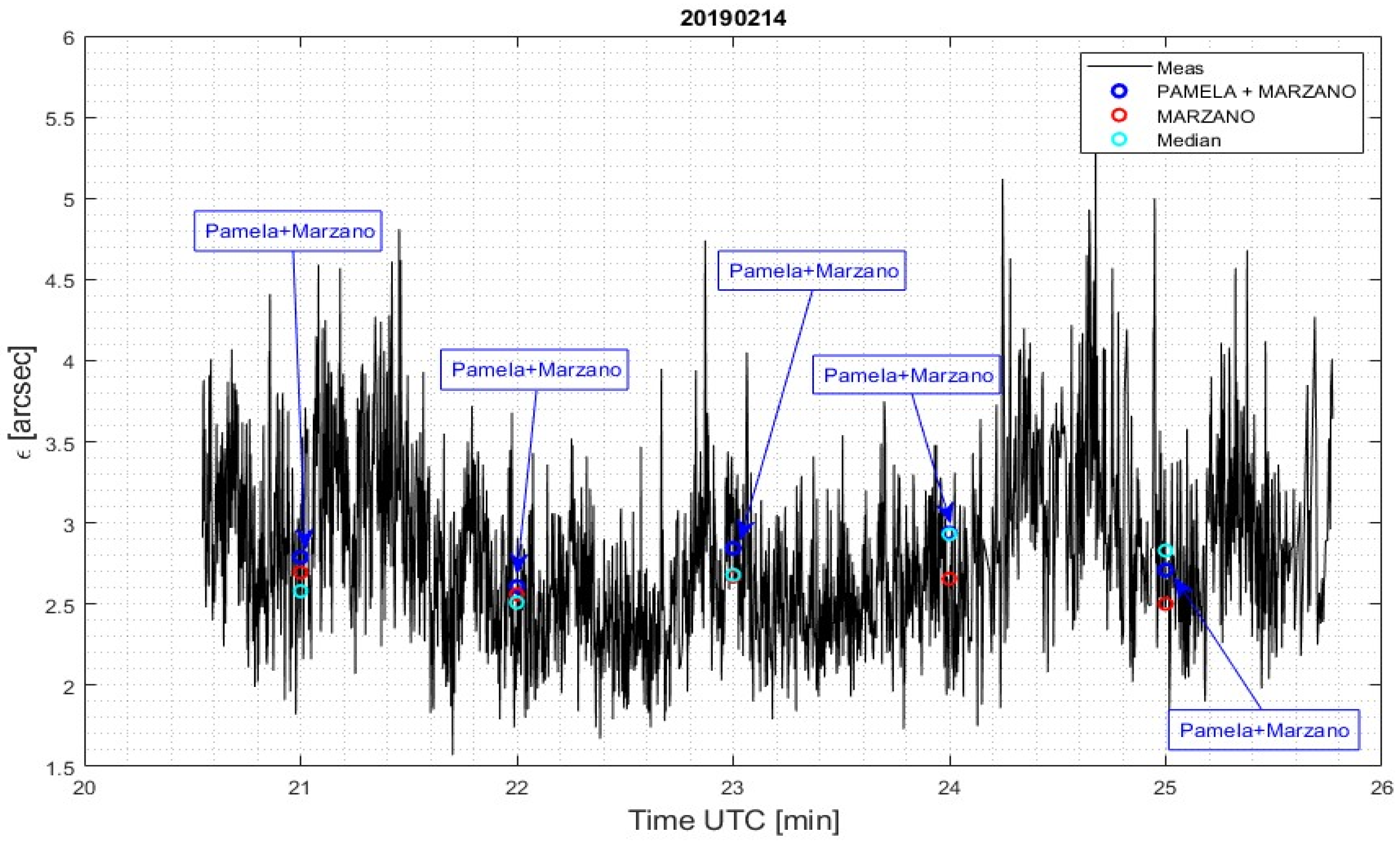
4. Data and Validation

Various datasets are collected, encompassing profiles of temperature, wind speed, astronomical parameters, and the refractive index parameter $C_n^2$. The meteorological data from the European Centre for Medium-Range Weather Forecasts (ECMWF) database and observations from the turbulence monitor (DIMM, differential image motion monitor instrument) form the foundation of these datasets. Within this section, we utilize ECMWF meteorological profiles as input to calculate seeing via $C_n^2$ models (Dewan, Trinquet–Vernin, Marzano, and Pamela). The aim is to compare these calculations with the seeing measurements taken in Redu, Belgium. The meteorological information employed includes the following: pressure, temperature, and wind profiles sourced from ECMWF. These profiles, available in the new fifth-generation ECMWF ReAnalysis (ERA5) database, feature a time resolution of 1 h. Derived through the assimilation of global meteorological measurements, these reanalysis data represent the most accurate and precise dataset accessible.

In the consideration of atmospheric turbulence models, it is essential to address the omission of certain models, such as the Hufnagel-Valley 5/7 model, from our study. The H-V 5/7 model, characterized as a non-parametric model, primarily emphasizes altitude in its calculations, rendering it highly site-specific. While this model has its merits in specific applications, we opted not to include it in our analysis. Our research aimed for a more comprehensive and parametric approach, seeking models that could provide a nuanced understanding of atmospheric turbulence across various conditions and locations. The Hufnagel–Valley 5/7 model, being more specialized and site-dependent, did not align with the broader scope of our study. Our choice of models, namely the Dewan, Marzano, Trinquet–Vernin, and Pamela models, was grounded in their ability to offer a more versatile and parametric representation of atmospheric turbulence under the specific conditions of our study area.

Matlab Simulation of $C_n^2$ and Seeing in Redu

For January and February 2019, this profile has been selected at the Redu location. In order to have a better grid point to calculate the $C_n^2$ models, the temperature measurement at nine different grid points based on ECMWF is compared in Figure 1. As is seen, the closest one to the Redu station is the red one (50.25 N, 5 E). Therefore, the designated grid point for Redu stands at 50.25 N, 5 E. A comparative analysis of the $C_n^2$ profiles and their associated four models (Dewan, Trinquet–Vernin, Marzano, and Pamela) is presented in the following section.

The following figures are generated based on ECMWF for the Redu station on 5, 6, and 14 February 2019 using Matlab simulation. Utilizing the grid point, we will conduct simulations for the seeing parameters. Figure 2 illustrates a comprehensive comparison of models alongside a measurement median for Redu on 5 February 2019. The dataset incorporates 419 recorded seeing values in Redu over approximately 100 min. In this section, we will employ the collected measurement data from Redu to assess our models and determine the model that best aligns with the observations. The lower $C_n^2$ values in Trinquet–Vernin’s model are the primary reason for the seeing values being lower than anticipated in comparison to other models. Additionally, Dewan’s model displays a more robust correlation with the measurement data (Meas), signifying its greater reliability.

Figure 3 displays Redu’s measurement median for 6 February 2019 alongside a comparison of all the available models. During a 360 min period, 1491 seeing values were documented in Redu. The Trinquet–Vernin model’s lower $C_n^2$ values naturally lead to lower seeing values compared to predictions from other models. Ultimately, empirical data supports the greater robustness of Dewan’s model.

Figure 4 presents a comparison between all existing models and the median of Redu measurements on 14 February 2019. Over a span of 310 min, a total of 2074 seeing observations were recorded in Redu. As anticipated, Trinquet–Vernin forecasts seeing values to be lower compared to other models, primarily because of the lower $C_n^2$ values it predicts. Ultimately, the empirical data lends support to the assertion that Dewan’s model is the most dependable.

As per (43), the calculation of the seeing can be separated into two components, which arise from the integration of the refractive index structure parameter in a particular manner:

By incorporating the Pamela model into the data analysis process, it can provide the accuracy of the measurements obtained from Redu station. The Pamela model’s capability to estimate the refractive index structure parameter $C_n^2$ within the surface boundary layer can complement the measurements taken in the free atmosphere, enhancing the comprehensiveness and reliability of the findings. This integration can offer a more comprehensive understanding of the optical turbulence phenomena occurring in the Earth’s atmosphere and contribute to the advancement of research in this field.

$$\varepsilon ={5.25{\lambda }^{-1/5}\left[\sec z{\int }_{h_0}^{h_0+L}{C}_n^2(h)dh\right]}^{3/5}$$

$$\varepsilon ={5.25{\lambda }^{-1/5}\left[\sec z{\int }_{h_0}^{h_0+h_{\mathit{bl}}}{C}_n^2(h)dh+{\int }_{h_0+h_{\mathit{bl}}}^{h_0+L}{C}_n^2(h)dh\right]}^{3/5}$$

$$\varepsilon ={5.25{\lambda }^{-1/5}\left[\sec z\left(I_{\mathit{bl}}+I_{\mathit{fa}}\right)\right]}^{3/5}$$

(44)

Taking $I_{\mathit{bl}}$ to represent the component arising from the boundary layer and $I_{\mathit{fa}}$ as the component originating from the free atmosphere, the calculation of the seeing parameter ($\varepsilon$) as per (44) can be decomposed into these two constituent parts. Given a linear correlation between ground and boundary layer height, the following equation can be established for $I_{\mathit{bl}}$:

$$I_{\mathit{bl}}={\int }_{h_0}^{h_{\mathit{bl}}}{C}_n^2\left(h\right)dh\approx {\left|C_{n,0}^2 - \left.C_{n,\mathit{bl}}^2\right|\right.}^{\frac{h_{\mathit{bl}}}{2}}$$

(45)

Given our understanding of the height of the atmospheric boundary layer in the region of Redu [29], the surface $C_{n,0}^2$ based on the Pamela model is simulated using the Matlab code with the ERA5 input data for Redu. Figure 5a,b illustrate the $C_{n,0}^2$ values at the surface for the entire days of 5–6 February 2019, respectively. Meanwhile, Figure 5c depicts the refractive index structure parameter $C_{n,0}^2$ for the surface on 14 February 2019.

The subsequent phase involves the utilization of these $C_{n,0}^2$ values to compute the contribution of the boundary layer to the seeing. To achieve this, the ERA5 input data are indispensable for simulating surface $C_{n,0}^2$ values via the Pamela model on 5, 6, and 14 February 2019 in Redu, as illustrated in Figure 5. Additionally, the well-established $C_{n,\mathit{bl}}^2$ values at the boundary layer height level from the Marzano and Dewan models for each respective date are necessary.

Once $I_{\mathit{bl}}$ is determined, the total seeing values (boundary layer + free space) and the seeing values (free space) are presented alongside measurements and their medians. Figure 6, Figure 7 and Figure 8 are based on the Dewan model, while Figure 9, Figure 10 and Figure 11 follow the Marzano model. These figures have been strategically arranged to provide a coherent narrative and facilitate a more comprehensive understanding of the impact of atmospheric turbulence on the overall seeing conditions.

This observation underscores the significant role of the boundary layer in influencing atmospheric seeing conditions. The incorporation of $I_{\mathit{bl}}$ into the models enhances the accuracy of representing the boundary layer’s impact on seeing quality. In the mentioned figures, it is evident that integrating $I_{\mathit{bl}}$ into the Marzano and Dewan models consistently improves seeing values, with the exception of 6 February 2019, which yields a higher estimate of seeing.

Overall, this contribution emphasizes the importance of considering boundary layer effects in atmospheric models to accurately assess seeing conditions. The results depicted in Figure 6, Figure 7, Figure 8, Figure 9, Figure 10 and Figure 11 provide compelling evidence that the inclusion of $I_{\mathit{bl}}$ in the Marzano and Dewan models enhances their predictive capabilities and advances our comprehension of atmospheric turbulence’s influence on astronomical observations.

5. Conclusions

To achieve an accurate assessment of atmospheric seeing, a comprehensive analysis encompassing the $C_n^2$ parameter across different atmospheric layers is imperative. This study relies on data from the European Centre for Medium-Range Weather Forecasts (ECMWF), particularly ERA5, to generate hourly profiles of atmospheric variables, including pressure, temperature, and humidity. These profiles are essential for computing the refractive index structure constant $C_n^2$ and assessing optical degradation.

The study meticulously selects a suitable grid point for temperature measurements at the Redu site based on ECMWF data. It employs various optical turbulence models like Dewan, Trinqut Vernin, Marzano, and Pamela to predict $C_n^2$ profiles, considering their accuracy under different atmospheric conditions. These models play a vital role in understanding and mitigating the impact of atmospheric turbulence on optical system performance. In summary, the Dewan model, similar to the Marzano model, is primarily applicable above the boundary layer, whereas Pamela is designed specifically for modeling within the boundary layer. Trinquet–Vernin, on the other hand, is tailored for the free atmosphere. A notable distinction lies in the formulation of the turbulence structure parameter, $C_n^2$. While the model based on Tatarski’s equation (Dewan, Marzano) uses $C_n^2$ proportional to ${\left(\frac{ d\theta }{ dh}\right)}^{ }$, Trinquet–Vernin diverges by having $C_n^2$ proportional to ${\left(\frac{ d\theta }{ dh}\right)}^2$. This difference in the power term alters the behavior of the model and its representation of turbulence characteristics, emphasizing the significance of understanding the nuanced variations among these models for accurate simulations. For an extended discussion on various $C_n^2$ models and non-Kolmogorov turbulence, kindly consult References [30,31].

Astronomical seeing [23,28], a crucial measure of star image blurring due to atmospheric turbulence, guides the validation process. To validate the chosen $C_n^2$ models, measurements from a DIMM (differential image motion monitor) are utilized in Matlab simulations. The study encompasses 3984 seeing measurements from ECMWF, covering February 2019 at the Redu station.

Figure 2, Figure 3 and Figure 4 provide substantial support for the accuracy of Marzano and Dewan models compared to the Trinquet–Vernin model, which predicts lower seeing values due to its lower $C_n^2$ values.

Assuming that we have knowledge of the atmospheric boundary layer’s height in Redu [29], determining the impact of this layer on seeing (referred to as $I_{\mathit{bl}}$) involves two essential steps. Firstly, we employ the ERA5 input data to generate surface $C_{n,0}^2$ values using the Pamela model [21]. Secondly, we must acquire the typical $C_{n,bl}^2$ values for 5, 6, and 14 February 2019, specifically for the Redu location. Incorporating $I_{\mathit{bl}}$, representing the boundary layer’s contribution, results in an elevation of seeing values for both the Marzano and Dewan models, as is clearly demonstrated in Figure 6, Figure 7, Figure 8, Figure 9, Figure 10 and Figure 11. This observation underscores the considerable influence exerted by the boundary layer on atmospheric seeing conditions. The integration of $I_{\mathit{bl}}$ into these models enables a more precise representation of the boundary layer’s impact on seeing quality. The figures consistently illustrate an enhancement in seeing values upon the inclusion of $I_{\mathit{bl}}$ into the models, except for 6 February 2019, for which a higher estimate of seeing is observed. This overall trend highlights the importance of accounting for the boundary layer’s effects when evaluating atmospheric seeing.

References

1. Bekhrad, P.; Ivanov, H.; Leitgeb, E. Car to X Communication with Optical Wireless as Support and Alternative to RF-Technologies for Roads and Future Transportation. In Proceedings of the IEEE 26th International Conference on Software, Telecommunications and Computer Networks (SoftCOM), Split, Croatia, 13–15 September 2018. [Google Scholar]
2. Majumdar, A.K. Advanced Free Space Optics (FSO): A Systems Approach, 1st ed.; Springer: New York, NY, USA, 2015. [Google Scholar]
3. The Radio Refractive Index: Its Formula and Refractivity Data. Available online: https://www.itu.int/dms_pubrec/itu-r/rec/p/R-REC-P.453-11-201507-S!!PDF-E.pdf (accessed on 1 January 2023).
4. Bean, B.R.; Dutton, E.J. Radio Meteorology; National Bureau of Standards: Boulder, CO, USA, 1966. [Google Scholar]
5. Tatarski, V.I. The Effect of the Turbulent Atmosphere on Wave Propagation; Israel Program for Scientific Translations: Jerusalem, Israel, 1971. [Google Scholar]
6. Ishimaru, A. Wave Propagation and Scattering in Random Media, Vol. 2 Multiple Scattering, Turbulence, Rough Surfaces and Remote Sensing; Academic Press: Cambridge, MA, USA, 1978. [Google Scholar]
7. Dewan, E.; Good, R.; Beland, B.; Brown, J. A Model for C n 2 (Optical Turbulence) Profiles Using Radiosonde Data; Phillips Laboratory: Bedford, MA, USA, 1993. [Google Scholar]
8. Dewan, E.; Grossbard, N. The inertial range “outer scale” and optical turbulence. Environ. Fluid Mech. 2007, 7, 383–396. [Google Scholar] [CrossRef]
9. Tatarski, V.I. Wave Propagation in a Turbulent Medium; Dover Publication, Inc.: New York, NY, USA, 1961; pp. 324–325. [Google Scholar]
10. Gurvich, A.S.; Kaprov, B.M.; Tsvang, L.; Yaglom, K. Empirical data on the small-scale structure of atmospheric turbulence. In Atmospheric Turbulence and Radio Wave Propagation; Nauka: Moscow, Russia, 1967; pp. 1–31. [Google Scholar]
11. Smith, F.G. Atmospheric Propagation of Radiation. In The Infrared & Electro-Optical Systems Handbook; SPIE Press: Bellingham, WA, USA, 1993; Volume 2, pp. 1–332. [Google Scholar]
12. D’auria, G.; Marzano, F.S.; Merlo, U. Model for estimating the refractive-index structure constant in clear-air intermittent turbulence. Appl. Opt. 1993, 32, 2674–2680. [Google Scholar] [CrossRef] [PubMed]
13. Bekhrad, P.; Leitgeb, E. Different models of the refractive index structure constant calculation. In Proceedings of the IEEE 3rd West Asian Symposium on Optical and Millimeter-Wave Wireless Communications (WASOWC), Tehran, Iran, 24–25 November 2020. [Google Scholar]
14. Marzano, F.S.; d’Auria, G. Model-based prediction of amplitude scintillation variance due to clear-air tropospheric turbulence on Earth-satellite microwave links. IEEE Trans. Antennas Propag. 1998, 46, 1506–1518. [Google Scholar] [CrossRef]
15. Ishimaru, A. Wave Propagation and Scattering in Random Media, Vol 1: Single Scattering and Transport Theory; Academic Press: Washington, DC, USA, 1978. [Google Scholar]
16. Vasseur, H. Prediction of Tropospheric Scintillation on Satellite Links from Radiosonde Data. IEEE Trans. Antennas Propag. 1999, 47, 293–301. [Google Scholar] [CrossRef]
17. Trinquet, H.; and Vernin, J. A statistical model to forecast the profile of the index structure constant C n 2 . Environ. Fluid Mech. 2007, 7, 397–407. [Google Scholar] [CrossRef]
18. Giordano, C.; Vernin, J.; Trinquet, H.; Munoz, C. Weather Research and Forecasting prevision model as a tool to search for the best sites for astronomy: Application to La Palma, Canary Islands. Mon. Not. R. Astron. Soc. 2014, 440, 1964–1970. [Google Scholar] [CrossRef]
19. Oh, E.; Ricklin, J.C.; Eaton, F.D.; Gilbreath, G.C.; Doss-Hammel, S.; Moore, C.I.; Murphy, J.S.; Oh, Y.H.; Stell, M. Estimating optical turbulence using the PAMELA model. Proc. SPIE 2004, 5550, 256–266. [Google Scholar]
20. Oh, Y.H.; Ricklin, J.C.; Oh, E.; Doss-Hammel, S.; Eaton, F.D. Estimating optical turbulence effects on free space laser communication: Modeling and measurements at ARL’s A_LOT facility. Proc. SPIE 2004, 5550, 247–255. [Google Scholar]
21. Ricklin, J.C.; Hammel, S.M.; Eaton, F.D.; Lachinova, S.L. Atmospheric channel effects on free-space laser communication. In Free-Space Laser Communications; Optical and Fiber Communications Reports; Springer: New York, NY, USA, 2006; Volume 2, pp. 9–56. [Google Scholar]
22. Van Der Graaf, S.C.; Kranenburg, R.; Seger, A.J.; Schaap, M.; Erisman, J.W. Satellite derived leaf area index and roughness length information for surface-atmosphere exchange modelling: A case study for reactive nitrogen deposition in north-western Europe using LOTOS-EUROS v2.0. Geosci. Model Dev. 2020, 13, 2451–2474. [Google Scholar] [CrossRef]
23. Hemmati, H. Near-Earth Laser Communications, 2nd ed.; CRC Press: Boca Raton, FL, USA, 2020; pp. 1–454. [Google Scholar]
24. Fried, D.L. Statistics of a Geometric Representation of Wave-front Distortion. J. Opt. Soc. Am. 1966, 55, 1427–1435. [Google Scholar] [CrossRef]
25. Giordano, C. Prediction et optimisation des techniques pour l’observation à haute resolution angulaire et pour la future generation de très grands telescopes. Ph.D. Thesis, Université Nice Sophia Antipolis, Nice, France, 2014. [Google Scholar]
26. Kemp, E.M.; Felton, B.D.; Alliss, R.J. Estimating the Refractive Index Structure-Function and Related Optical Seeing Parameters with the WRF-ARW. In Proceedings of the 9th WRF User’s Workshop, NCAR, Boulder, CO, USA, 23–27 June 2008. [Google Scholar]
27. Nelson, D.H.; Walters, D.L.; MacKerrow, E.P.; Schmitt, M.J.; Quick, C.R.; Porch, W.M.; Petrin, R.R. Wave Optics Simulation of Atmospheric Turbulence and Reflective Speckle Effects in CO2 Lidar. Appl. Opt. 2000, 39, 1857–1871. [Google Scholar] [CrossRef] [PubMed]
28. Liu, L.Y.; Giordano, C. Optical Characterization at LAMOST Site: Observation and models. Mon. Not. R. Astron. Soc. 2014, 451, 3299–3308. [Google Scholar] [CrossRef]
29. Bekhrad, P. Evaluation of the Refractive Index Structure Constant Profile and Seeing. Ph.D. Thesis, Graz University of Technology, Graz, Austria, 2023. [Google Scholar]
30. Andrews, L.C.; Phillips, R.L. Laser Beam Propagation through Random Media, 2nd ed.; SPIE Press: Bellingham, WA, USA, 2005; Volume PM152, pp. 1–808. [Google Scholar]
31. Zilberman, A.; Golbraikh, E.; Kopeika, N.S. Propagation of electromagnetic waves in Kolmogorov and non-Kolmogorov atmospheric turbulence: Three-layer altitude model. Appl. Opt. 2008, 47, 6385–6391. [Google Scholar] [CrossRef] [PubMed]
Figure 1. A comparative analysis of 2 m temperature data from the nine nearest points to the Redu station in February 2019.
Electronics 13 00055 g001
Figure 2. Simulation of astronomical seeing using three models contrasted with measurements (means) in Redu on 5 February 2019 at 00:00:00 UTC.
Electronics 13 00055 g002
Figure 3. Comparative seeing simulations for the three models against Redu measurements on 6 February 2019, at 00:00:00 UTC as per ECMWF data.
Electronics 13 00055 g003
Figure 4. Simulation of seeing for three models, juxtaposed with measurements taken in Redu on 14 February 2019 using ECMWF data at 00:00:00 UTC.
Electronics 13 00055 g004
Figure 5. The surface value of C n , 0 2   for the entire day on (a) 5 February, (b) 6 February, and (c) 14 February 2019 in Redu.
Electronics 13 00055 g005
Figure 6. Total seeing values (boundary layer + free space) compared to ERA 5 input data (blue) and typical C n 2   values (in free space) (red) based on Dewan, along with measurements and median, on 5 February 2019 in Redu.
Electronics 13 00055 g006
Figure 7. Total seeing values (boundary layer + free space) compared to ERA 5 input data (blue) and typical C n 2 values (in free space) (red) based on Dewan, along with measurements and median, on 6 February 2019 in Redu.
Electronics 13 00055 g007
Figure 8. Comparison between the total seeing values (boundary layer + free space) with ERA 5 input data (blue) together with typical C n 2 values (in free space) (red) based on Dewan model, along with measurements and median, on 14 February 2019 in Redu.
Electronics 13 00055 g008
Figure 9. Total seeing values (boundary layer + free space) compared to ERA 5 input data (blue) and typical C n 2 values (in free space) (red) based on Marzano, along with measurements and median, on 5 February 2019 in Redu.
Electronics 13 00055 g009
Figure 10. Total seeing values (boundary layer + free space) compared to ERA 5 input data (blue) and typical C n 2 values (in free space) (red) based on Marzano, along with measurements and median, on 6 February 2019 in Redu.
Electronics 13 00055 g010
Figure 11. Comparison between the total seeing values (boundary layer + free space) with ERA 5 input data (blue) together with typical C n 2 values (in free space) (red) based on Marzano model, along with measurements and median, on 14 February 2019 in Redu.
Electronics 13 00055 g011