
A Model Predictive Control Algorithm for the Reconfiguration of Radially Operated Grids with Islands


1
Department of Computer, Control and Management Engineering (DIAG), University of Rome “La Sapienza”, Via Ariosto, 25, 00185 Rome, RM, Italy
2
Faculty of Engineering, eCampus University, Via Isimbardi, 10, 22060 Novedrate, CO, Italy
*
Author to whom correspondence should be addressed.
Electronics 2023, 12(24), 4982; https://doi.org/10.3390/electronics12244982
Submission received: 8 October 2023
/
Revised: 1 December 2023
/
Accepted: 7 December 2023
/
Published: 12 December 2023
(This article belongs to the Special Issue Section Collection Series: New Horizons and Recent Advances in Power Electronics)
Abstract
:This paper proposes a reconfiguration algorithm for electricity grids, based on Model Predictive Control (MPC). Reconfiguration is dynamically performed to reduce losses, and in reaction to adverse events, such as faults or attacks. Most of the previous works in the literature (including a previous paper from the authors) focus on the reconfiguration of grids while ensuring they are always radially operated and connected (i.e., islands are not allowed to form). At present, including the possibility of performing a dynamic islanding of the network (i.e., where portions of the grid dynamically detach and reconnect to the main grid) is seen as a way to improve the flexibility and resiliency of the grid, especially in the present context, with the increased penetration of digital technologies and renewables. Therefore, by extending the previous work, the algorithm proposed in the present paper also allows for the formation of islands, while still constraining them to radial islands, in line with the operational practice adopted by most electric companies. The mathematical formulation of the grid reconfiguration problem is discussed, and simulation results are presented, showing the effectiveness of the proposed algorithm in dynamically managing the grid reconfiguration.
1. Introduction
Transmission and distribution grids are increasingly characterized by the presence of distributed energy resources, such as electric energy storage systems (ESS), renewable energy plants, and plug-in electric vehicles. This paradigm shift from passive and centralized energy systems of the past presents numerous challenges in terms of the increased complexity of operations. Among other factors, the variability in the power production from renewable plants and the intermittency of PEVs demand require the continuous control and optimization of the grid. Among the available means of control, grid reconfiguration is acknowledged as one of the degrees of freedom available to balance the grid load, reduce grid losses, and quickly restore the service after disruptions to the grid [1]. While reconfiguration was performed offline in passive grids, it can now be performed more often during the day to dynamically optimize the grid following its evolving boundary conditions. In this paper, we describe a reconfiguration algorithm based on model predictive control (MPC), whose goal is to dynamically reconfigure the grid in order to minimize losses when facing adverse events such as faults. The paper extends our previous work [2] by removing the requirement that the grid be connected at all times. In the present version, the algorithm also allows for the formation of islands in the grid, which is a natural scenario in the future, where it is expected that microgrid islands will be able to dynamically connect and disconnect from the grid.
1.1. Literature Survey and Contributions
Network reconfiguration algorithms play a crucial role in enhancing the efficiency and resiliency of modern electric grids. Indeed, changes in the grid topology can reduce power losses, improve voltage profiles and stability, balance loads, and mitigate the impact of faults and attacks [3]. Many network reconfiguration approaches have been proposed in the literature and can be classified in classic optimization-based, (meta) heuristics (including evolutionary algorithms) and machine-learning-based solutions. With respect to the other algorithms, the former class of algorithms has the advantages of allowing for an optimal solution to the reconfiguration problem to be found, as well as explicitly considering constraints and optimizing the provided optimality criteria. However, this often comes at the price of high computational costs. On the other hand, (meta)heuristics are characterized by lower computational costs but do not guarantee the optimality of the reconfigured topology. Machine Learning (ML), particularly Reinforcement Learning (RL), techniques represent a promising research line in the context of network reconfiguration for large-scale systems due to their ability to infer (near) optimal policies. As an example, in [4], the authors address the dynamic distribution network reconfiguration, proposing a Deep Reinforcement Learning algorithm. The proposed solution relies on a reduced action space allowing for the artificial agent to only select configurations that satisfy radiality constraints. The objective function aims to minimize the costs associated with the active energy loss and the manipulation of switching devices. In [5], the authors propose an RL algorithm that is able to learn the network reconfiguration control policy based on historical data. The same approach was adopted in [6], in which the authors train an off-policy RL agent using historical data. Said data are further increased by means of data augmentation techniques, allowing for the training to be implemented on a larger data set. Although these techniques avoid relying on exact models of the distribution network, they have some drawbacks. Indeed, it should be noted that the training phase required by the (D)RL approaches may require significant computational effort. In this respect, in [7] the authors compared several DRL algorithms with classic optimization-based heuristics and genetic algorithms. The results showed how DRL techniques are characterized by significantly lower computational times (especially when the dimensions of the considered scenario increase) but require long training phases. Another issue with ML-based approaches is represented by the fact that they do not explicitly consider constraints. In this respect, there are some works that tackle this issue, proposing safe learning techniques. In [8], for example, the authors adopt the Deep Deterministic Policy Gradient (DDPG) algorithm to learn the control policies. Safety is implemented by means of a layer allowing for the prediction of changes in the constrained states, preventing the violation of operational constraints. However, as was also pointed out by the authors, in the context of network reconfiguration problems, RL-based techniques should be used wisely. Indeed, it is shown that the control performances of MPC techniques are in line with those of the proposed DRL algorithm. Since DRL algorithms require a significant effort in the tuning of hyperparameters and the shaping of the reward functions, the added complexity may not be worthwhile compared to the small improvement in performance. Furthermore, distribution networks may be composed of devices operating in a continuous and/or discrete way. This means that different DRL techniques should be adopted in different scenarios, since not all algorithms can deal with continuous and/or discrete state and action spaces. Finally, it should be also noted that RL algorithms are trained on specific instances: if such training scenarios are not representative of new, unforeseen scenarios, the learned policy may be not effective.
Motivated by these considerations, the solution proposed in this work to tackle the network reconfiguration problem is based on MPC, which is an optimization-based technique retaining the advantages of optimal control-based approaches. As discussed in Section 4, the proposed MPC approach guarantees low computational costs, making it suitable for real-time applications. MPC is a closed-loop optimization technique, which has been widely adopted, especially in the industrial sector. Surprisingly, in the context of network reconfiguration, MPC has not been extensively adopted [1] although there are some interesting works in the literature. In [9], for example, the author considers a distribution network composed of several distribution feeders and tackles the problem of network reconfiguration with the goal of minimizing the operating costs. The proposed solution, based on a Stochastic MPC, proves to be able to reduce energy losses and to induce a certain degree of robustness in the network with respect to the variable power generation peculiar of Renewable Energy Sources (RESs) and prediction errors. A Stochastic MPC was also proposed in [10], in which the authors tackle the problem of scheduling operations and reconfigure switches in a distribution network. The proposed solution aims to minimize the total operating costs and embed technical constraints (e.g., ESSs’ limits, power flow equations, bus and lines capacities), minimize topology constraints, and also establish a demand–response model. The authors also discuss the trade-off between computational costs and performances (i.e., cost reductions), which depends on the dimension of the considered time horizon. In [11] the authors adopt a similar methodology to simultaneously address the network reconfiguration and Plug-in Electric Vehicles’ (PEVs’) charging management problems. The proposed stochastic MPC aims to minimize the operating costs of the distribution network (including the costs associated with changes in the network configuration) and of the PEVs’ charging. In [12], the authors address an interesting generalization of the network reconfiguration problem, simultaneously considering the distribution network, grid actuators and buildings. The authors propose a centralized MPC to optimize the power flow of the distribution network while guaranteeing thermal comfort in the buildings. An interesting work in the context of MPC algorithms applied to reconfiguration problems is [13], in which the authors consider networked cyber–physical systems. Although the application domain and the considered control problem are not in line wih the subject of this work, the proposed distributed MPC implementation could be interesting for future development. Topology changes in large networked systems are also addressed in [14], in which the authors propose a distributed MPC that is able to guarantee the feasibility of the control actions taken by the local controllers.
The main contribution of this paper is the investigation of grid reconfiguration, also considering the possibility of the dynamical formation of islands in the grid. To achieve this, the formulation of the previous work [2] was extended with new radiality constraints that also allow for the formation of islands. Also, the power flow equations are integrated by following the conic programming approach presented in [15,16], which is slightly modified here by the addition of simple constraints (14) and (15), which state the symmetric and anti-symmetric properties of two variables appearing in the power flow equations. Their addition helps the solver to find the correct solution.
Regarding radiality, different radiality constraints have been proposed in the literature. In [17], in which 0 denotes the closed state for a switch and 1 the open one, radiality is imposed by forcing the sum of the state of all the switches to one along every loop in the network. In this way, one switch in every loop is open, and thus the network is radial. In [18], in which one substation is considered, the list of all possible paths from every node to the substation is computed. Then, radiality is enforced by constraining every node so that only one such path is active, and also by forcing that, if a path is active, all the paths contained in that path are also active (recall that a path is defined in [18] as a sequence of links connecting a given node to the substation). In [19], Romero-Ramos et al. propose using a simple equation that constrains the sum of the status of all the links (which is equal to one if the link is closed) to be equal to the number of non-substation buses in the network. This equation is later used in [12]. The authors of [19] explain that this simple equation fails to impose radiality when there are non-injection buses in the network (since they can remain disconnected, and loops can then form). To solve this issue, they include constraints to force the existence of at least one active path between every zero-injection bus and a non-zero-injection bus. A similar strategy is adopted in [10], in which additional constraints are included to force every node to have one parent node. An alternative method for checking the radiality of a strongly connected grid (i.e., with no islands) is presented in [20], based on a calculation of the determinant of the connection matrix. This method is used, for example, in [11]. In this paper, we write the radiality constraints so that they also work in the islanded case, i.e., they allow for the formation of radial islands in the grid. To the best of our knowledge, the other work considering the formation of dynamic islands is [21], which proposes different and more complex equations than the ones presented here.
The relevant features of the key papers discussed above are outlined in Table 1.
1.2. Paper Structure
The remainder of the paper is organized as follows. The next section presents the reference scenario of the study, and the MPC control logic. Section 3 presents the formulation of the proposed MPC reconfiguration algorithm, detailing the problem constraints and the objective function. Section 4 presents the simulations performed to validate the approach, considering a grid equipped with ESS and renewable plants. Finally, Section 5 reports the conclusions and the proposed future works.
2. Reference Scenario and Proposed MPC Approach
The reference scenario focuses on the control of an electricity grid whose topology can be dynamically changed to improve the performance of the network (e.g., to minimize losses), and also to face adverse events such as faults.
The reference scenario is depicted in Figure 1. The reconfiguration of the grid is controlled with a centralized MPC algorithm. MPC is widely adopted in any industry, thanks mainly to its ability to handle constrained control, and the possibility it offers to optimize relevant key performance indicators through the design of the objective function. For a throughput discussion of the MPC control technique, the reader is referred to one of the main reference books in the field, e.g., [22]. A brief description of the MPC control logic is described in Algorithm 1, and discussed in the following. The control is in discrete time; T denotes the sampling time. At the beginning of the generic time step k, the MPC algorithm acquires all the information about the current state of the grid (including the energy level of the storage and the current configuration). Then, an optimal reconfiguration optimization problem (also known as “the MPC iteration”) is built and solved. The optimization problem is composed of an objective function, which captures the need to minimize energy losses, and several constraints, to ensure that the reconfiguration actions that are computed are admissible, and that all the variables (voltage magnitudes, angles, etc.) remain within the safety limits. The formulation of such an optimization problem, in terms of the objective function and the constraints, is presented in the next Section. At every time step, the solution of the optimization problem contains the optimal commands to send to the grid, which include the status of every switch and the power injection/consumption of the storage.
| Algorithm 1 MPC charging sessions’ control algorithm |
|
The nomenclature used in the paper is listed in Table 2.
The electricity grid is modelled as a graph , with a set of nodes (or vertices) and a set of links . Use to denote the set of nodes that, in , are physically connected to node i, i.e., . Links in can generally be connected and disconnected by acting on breakers and switches. We model this control action through the inclusion of a Boolean variable associated with the generic link . For convention, the variable is equal to one if the link is connected and equal to zero if the link is disconnected (it is, of course, at all times). For the links that are not equipped with breakers or switches, the value of is constrained to one for all the times. Then, at any generic time, depending on the status of the switches, the current network topology of the grid might differ from .
For this reason, we refer to as the physical topology, to distinguish this from the specific topology to which the grid might be configured at a generic time k, which is denoted with . Similarly to , let denote the set of nodes that is directly connected to node i at time k. In general is a highly meshed network, while we want to ensure that the reconfiguration algorithm proposed in this paper makes sure that does not contain cycles. In particular, might be a disconnected network (i.e., it might contain islands), but any island must be operated radially, which is a standard requirement for the operation of distribution grids.
In the next section, the optimization control problem built and solved in line 3 of Algorithm 1 is described. This optimization problem belongs to the category of mixed-quadratic-integer problems, since it has quadratic terms in the objective function, and it has both continuous and integer (Boolean in this case) variables. Standard solvers exist to solve such problems.
3. Proposed MPC Reconfiguration Algorithm
In the following, we detail the mathematical formulation in terms of the objective function and constraints of the optimization problem that is solved at each instant k by the MPC controller (step 3 in Algorithm 1) over the time interval , the well-known control horizon. Hereafter, thestandard notation for the power system is used: is the bus power injection (positive) or withdrawal (negative), and denote the active and reactive line power flows of the line connecting buses i and j, is the bus voltage, is the bus voltage angle, and represents the difference between voltage angles at buses i and j. Power injection and withdrawal at each bus are named , , and .
3.1. Objective Function
The objective function is designed to minimize the system power losses and the switching actions, and to keep the ESSs state of charge close to a convenient reference value, to guarantee they always have a margin of intervention. The index is used to indicate a generic time instant within the control horizon. The objective function is given by:
The subscript N in indicates that the optimal control problem is defined over N prediction time intervals, denotes the state of the controlled variable at instant k, and is the set of control variables, i.e., the ESS power injection and the switching actions . Parameters are the objective function weights. The first term is the sum of the power injected/withdrawn at every bus in the grid. This represents the total power loss in the network, which has to be minimized. The second term is a tracking term aiming to maintain the average state of charge of the ESS at close to the reference value. This should avoid the ESSs being either fully charged or fully depleted at any point in time (a situation that should be avoided since, in that case, they could not be either charged or discharged). The third term is used to control the number of feeders connections/disconnections, to avoid new configurations being calculated too often.
3.2. Power Flow Constraints
The following constraints are added to the above objective function for . Starting from the well-known nonlinear power flow equations (e.g., [15]), the active and reactive power flows from node i to node j are:
where . Elements and are the line series conductance and susceptance, i.e., the real and the imaginary parts of the line series admittance . Lines’ shunt elements are neglected (a reasonable assumption in distribution networks [23]). Equations (2) and (3) are defined for line such that . To exactly linearize the equations, additional auxiliary variables and constraints are introduced. Specifically, let us introduce variables for and and for each line , defined as follows [16]:
The variables and are defined for each line , and and are defined at network nodes i and j. Variables are non-negative, since they are intended to model the product of voltage times and the cosine of the angle (see (4)):
Following [16], to model the configuration variables within the power flow equations, it is necessary to introduce two additional control variables, and , for each distinct line , and the following constraints were used:
Variables and are zero when the line is disconnected (i.e., ; see Equations (6) and (7)), and equal and , respectively, when the line is connected (i.e., ; see Equations (8) and (9)). The relationship between the variables introduced above is given as follows (see (33) in [16]):
With the new variables shown above, after some manipulation (details in [16]), the power flow Equations (2) and (3) assume the linearized form in terms of these new variables:
Note that, from the above equations, when a line is disconnected it is and , as expected.
For each node, in terms of the new variables, the voltage limits are:
The following relations are introduced, which come from (4) and are important to ensure that the transformation is consistent
For each substation, we set [15]
where is set at 1 pu.
The ESS are modeled by the following equations:
where and represent the active and reactive power of ESS connected at bus i. is the measured ESS energy that is stored, T is the discretization time step, and the initial conditions at each instant of k are
where is the measured ESS energy stored at instant k. The power-balance equations for all the nodes are:
where is the power injected by the HV/MV substations, is the power injected by all the distributed generations at the respective node, and are the neighbour nodes of node i. Finally, to prevent non-injection buses from remaining isolated, the following constraint is introduced
which means that each node has to be connected with at least one other node. The control variables are and .
3.3. Radiality Constraints
The radiality constraints are modified with respect to our previous work [2]. They are needed to correctly guide the reconfiguration algorithm, to make sure that the proposed configurations do not contain loops, which is not desired in current network operation practice by the system operators. In this work, we still enforce radiality, but we make it possible for the algorithms to let islands form when convenient, e.g., to deal with a fault.
To ensure that every island in the network is radial, the following constraints are added:
where is any subset of of cardinality greater than 2. In fact, it is intuitive that a connected graph with nodes only has loops if there are edges in the graph. As discussed in [24], writing the above constraint only for is not sufficient, as this allows for the formation of islands with loops (see, e.g., Figure 4 in [24]). However, by including the above constraint (i.e., for every subset in ), we make sure that every island (which can be viewed as a subset of nodes of ) has no loops. One potential drawback of the use of (25) is that the number of constraints that need to be added grows exponentially with the size of the network. Specifically, the number of constraints to be added is equal to the number of subsets of nodes of with a cardinality greater than 2 (indeed, notice that there cannot be loops in subsets with only two nodes):
In practice, however, the number of constraints (25) to be added is much lower than (26), since it is not necessary to consider subsets that are disconnected in the physical topology, or that are connected in the physical topology by a lower number of links than (since it is not possible to form loops in this case).
In conclusion, constraint (25) is added only for the subsets satisfying the following condition:
which means that it is only added for the subsets of nodes that are connected (in the physical topology) by a number of links greater than .
4. Simulations
We simulate one day of network operation to show how the combined use of ESSs and reconfiguration actions can efficiently manage the grid in nominal and adverse conditions, simulating faults/(cyber)attacks.
4.1. Simulation Setup
Simulations were performed in Julia 1.8.5 [25]. The MPC iterations were solved with the solver Gurobi [26]. The PC was equipped with Intel i7-8565U @1.8 GHz and 16 GB RAM, running Windows 11.
The chosen grid was the 16-bus, three-feeder distribution network, and network data were chosen from [27], to which we added both generation and ESS devices and also some branches to increase the network configuration capability (see Figure 2).
Specifically, the bus types were as specified in Table 3 and network electric parameters are summarized in Table 4.
As explained in [16], the substation voltages were fixed at 1.0 pu and the minimum allowed load voltage was 0.95 pu. The sampling time was set to minutes and the MPC prediction horizon was set to . The weights of the Equation (1) were chosen empirically to be equal to , and . Note the orders of magnitude of difference between and the other weights; the reason for this is to achieve a more controlled focus on power loss reduction. The parameter was chosen to be small enough to guarantee the successful activation of ESSs; in fact, increasing means that the controller tries to keep the ESS stored energy close the reference value, consequently discouraging its activation. The value of was chosen to guarantee a good performance while limiting the number of configurations. The MV busbars of the HV/MV substations are characterized by the small and constant power consumption of 10 kW, characterizing the device consumption necessary for the operation of the network. The distributed simulated power generation hosted by the buses is represented in Figure 3 with a peak of 750 kW during the hottest hours of the day, and shifted over time to simulate a real and different geographical position.
The simulated bus loads have a steps shape and differ from each other only in terms of magnitude (see Figure 4). The reason for choosing these types of functions is to stress the system with sudden changes in load. This is particularly useful when testing non-nominal conditions and can verify the robustness of the mathematical model and prove if and how the system is able to respond to adverse events.
All measures are represented per unit to avoid numerical issues, and to convert the electrical values of the network into per-unit measurements, we considered the base power of 62 MW and the base voltage of 24 kV as the nominal power and voltage of the equipment, respectively.
At each bus, the maximum and minimum voltage values were set to kV and kV (i.e., 95% of ). The transmission power constraints of substations were chosen as follows: MW, MW and MVA, MVA for active and reactive power, respectively. Power bus constraints were MW, MW and MVA, MVA. The line power constraints were MW, MW and MVA, MVA.
The ESS energy reference was set to be equal to of total ESS capacity. All the ESSs had a maximum capacity of 2 MWh.
All branches were assumed to be configurable, i.e., equipped with switches. Note that, in real cases, this assumption could be relaxed because the network could contain some fixed and non-configurable branches.
The Equation (25) was implemented using a customised version of the Depth-First Search (DFS) algorithm whose computational time, in the worst case, is linear and corresponds to the size of the graph , where is the number of vertices and is the number of edges. It is also linear in terms of space regarding the number of vertices in the worst case.
4.2. Simulation of Normal Conditions
In this section, the simulations under normal conditions are presented, i.e., when no faults occur. Figure 5 depicts the computed configurations in nominal conditions. The starting configuration (graph topology) was set with all opened branches. In the first iteration, the algorithm chooses to close some branches, depicted at time 0:00. During the simulation time of 24 h, four reconfigurations are computed.
The power flow of all lines is depicted in Figure 6, where a generic line refers to the connection between bus i and bus j, with , e.g., L16, serving as the line connecting buses 15 and 16. Figure 7 shows the power flow of line 16 in detail. In this case, both flows described by the power flow equations are shown, from bus i to bus j and vice versa.
The behaviors of the power and energy stored by ESSs are shown in Figure 8 and Figure 9, respectively. ESSs at buses 7 and 9 are always an active part of the network. First of all, they are located in a sensible part of the network. ESS 7 has to feed the tree of the network, which is disconnected from any DG, it has to feed a large tree, and it is also located away from the primary substation. After 12:00 and 18:00, its role is to power the largest tree in the network. ESS 3 is never activated, as expected, because it is directly connected to the HV/MV substation.
Simulations were also carried out by setting and obtaining 79 reconfigurations.
4.3. Simulation of Adverse Event
This section presents the case in which, at some point, time faults/(cyber-)attacks occur, causing the algorithm to calculate a new configuration to counteract the lack of faulty lines or adverse events in general. For this purpose, the fault in the lines is presented in Table 5, where a faulty line is disconnected from the network and its recovery is assumed to take no less than 24 h, i.e., the fault is permanent for the entire duration of the simulation.
Seven reconfigurations occur; some of them are depicted in Figure 10. The configuration computed at the first iteration is not plotted and does not change until 7:30, when a new configuration is calculated. Notice that the intention is to force the formation of an island simulating the failure of lines described in Table 5. The island formed at 20:00.
Figure 11 and Figure 12 depict the energy and power of each ESS; the vertical lines highlight the time steps at which faults occur. Also, in this case, the weights of the objective function were chosen to encourage the use of ESSs. As expected, ESS 3 was not activated because of its proximity to the HV/MV substation. ESS 7, at 20:00, comes into play in a more decisive way because it has to feed the island.
In Figure 13, the power flows of line 16 (L16) are reported and it becomes inactive due the reconfigurations that occur from 14:45 to just before 20:00, as per Figure 10.
A general overview of the power flows along all the lines is reported in Figure 14. Note that the only difference from the normal case scenario is that, here, the simulations were carried out by setting a constant load of 50 kW connected to bus 7. This is because the island is fed by only an ESS and a DG; therefore, the power available to counteract the load is limited. In this specific case, a high level of consumption makes the problem unfeasible, as expected.
To demonstrate the effectiveness of the third term in the objective function, simulations were also carried out with , obtaining 63 reconfigurations.
4.4. Benchmark and Power Losses Considerations
The last consideration regards the power losses, and the simulations of Section 4.2 and Section 4.3 are compared with the case in which the network is static, i.e., no reconfiguration occurs. To this end, the reference scenario is the one depicted in Figure 2, in which links with solid lines are considered fixed links and the ones with dotted lines are always considered open (). Losses are simply calculated as the sum of the power injections at each bus. Figure 15 and Figure 16 show losses in the static scenario, and the total mean loss is 4.9%.
Figure 17 and Figure 18 show losses in the normal conditions scenario, and the total mean loss is 4.6%.
Figure 19 and Figure 20 show losses in the adverse events scenario, and the total mean loss is 5.01%.
The results clearly show how the present reconfiguration algorithm is better in terms of loss optimization compared to the benchmark solution given by a completely static network.
4.5. Computational Complexity
5. Conclusions and Future Works
This paper presented a Model Predictive Control (MPC) approach to the dynamic reconfiguration of electricity grids. The proposed mathematical formulation is extended from a previous paper by the authors, allowing for the dynamic formation of islands fed by ESS and local plants, which help the grid to reduce losses, and allow for better reconfigurarion following faults and adverse events. Also, during islanding, the radial operation of the entire grid is guaranteed by the inclusion of dedicated radiality constraints (which also guarantee the radiality of all the islands). Simulations are performed to test the algorithm in normal and adverse conditions, when faults occur on the lines. The results show the positive interplay between the ESS action and reconfiguration, which the algorithm can ensure in order to minimize dynamic losses and react to faults through the dynamic formation of islands.
Future works will deal with the extension of the algorithm so that it can manage notifications about the future expected level of risk for all the network components, and react to cyberattacks that are detected or predicted based, e.g., on network traffic analysis or other means. In addition, real-time simulations will be performed to accurately model the dynamics of the network during switching and evaluate the performance of the controller in a real-time implementation, i.e., also considering the impact of the MPC computation time compared to the sampling time.
Author Contributions
Conceptualization: M.D., A.D.G. and F.L.; Formal analysis: M.D., A.D.G. and F.L.; Investigation: M.D., A.T., A.D.G. and F.L.; Methodology: M.D., A.T., A.D.G. and F.L.; Project administration: F.L.; Resources: F.L.; Software: M.D. and F.L.; Supervision: A.D.G. and F.L.; Validation: M.D., A.T., A.D.G. and F.L.; Visualization: M.D.; Writing—original draft: M.D., A.D.G. and F.L.; Writing—review and editing: M.D., A.T., A.D.G. and F.L. All authors have read and agreed to the published version of the manuscript.
Funding
This research received no external funding.
Institutional Review Board Statement
Not applicable.
Informed Consent Statement
Not applicable.
Data Availability Statement
Data are contained within the article.
Acknowledgments
The authors gratefully acknowledge the anonymous reviewers.
Conflicts of Interest
The authors declare no conflict of interest. The funders had no role in the design of the study; in the collection, analyses, or interpretation of data; in the writing of the manuscript, or in the decision to publish the results.
Abbreviations
The following abbreviations are used in this manuscript:
| DG | Distributed Generation |
| ESS | Energy Storage System |
| HV | High Voltage |
| LV | Low Voltage |
| MV | Medium Voltage |
| MPC | Model Predictive Control |
| PEV | Plug-in Electric Vehicle |
| RES | Renewable Energy Source |
References
- Aziz, T.; Lin, Z.; Waseem, M.; Liu, S. Review on optimization methodologies in transmission network reconfiguration of power systems for grid resilience. Int. Trans. Electr. Energy Syst. 2021, 31, e12704. [Google Scholar] [CrossRef]
- Liberati, F.; Di Giorgio, A.; Giuseppi, A.; Pietrabissa, A.; Delli Priscoli, F. Efficient and risk-aware control of electricity distribution grids. IEEE Syst. J. 2020, 14, 3586–3597. [Google Scholar] [CrossRef]
- Mishra, A.; Tripathy, M.; Ray, P. A survey on different techniques for distribution network reconfiguration. J. Eng. Res. 2023, in press. [Google Scholar] [CrossRef]
- Kundačina, O.; Vidović, P.M.; Petković, M. Solving dynamic distribution network reconfiguration using deep reinforcement learning. Electr. Eng. 2022, 104, 1487–1501. [Google Scholar] [CrossRef]
- Gao, Y.; Wang, W.; Shi, J.; Yu, N. Batch-Constrained Reinforcement Learning for Dynamic Distribution Network Reconfiguration. IEEE Trans. Smart Grid 2020, 11, 5357–5369. [Google Scholar] [CrossRef]
- Gao, Y.; Shi, J.; Wang, W.; Yu, N. Dynamic Distribution Network Reconfiguration Using Reinforcement Learning. In Proceedings of the 2019 IEEE International Conference on Communications, Control, and Computing Technologies for Smart Grids (SmartGridComm), Beijing, China, 21–23 October 2019; pp. 1–7. [Google Scholar] [CrossRef]
- Gholizadeh, N.; Kazemi, N.; Musilek, P. A Comparative Study of Reinforcement Learning Algorithms for Distribution Network Reconfiguration with Deep Q-Learning-Based Action Sampling. IEEE Access 2023, 11, 13714–13723. [Google Scholar] [CrossRef]
- Kou, P.; Liang, D.; Wang, C.; Wu, Z.; Gao, L. Safe deep reinforcement learning-based constrained optimal control scheme for active distribution networks. Appl. Energy 2020, 264, 114772. [Google Scholar] [CrossRef]
- Rahmani-Andebili, M. Dynamic and adaptive reconfiguration of electrical distribution system including renewables applying stochastic model predictive control. IET Gener. Transm. Distrib. 2017, 11, 3912–3921. [Google Scholar] [CrossRef]
- Esmaeili, S.; Anvari-Moghaddam, A.; Jadid, S.; Guerrero, J.M. A Stochastic Model Predictive Control Approach for Joint Operational Scheduling and Hourly Reconfiguration of Distribution Systems. Energies 2018, 11, 1884. [Google Scholar] [CrossRef]
- Rahmani-Andebili, M.; Fotuhi-Firuzabad, M. An Adaptive Approach for PEVs Charging Management and Reconfiguration of Electrical Distribution System Penetrated by Renewables. IEEE Trans. Ind. Inform. 2018, 14, 2001–2010. [Google Scholar] [CrossRef]
- Zhang, Y.; Qian, T.; Tang, W. Buildings-to-distribution-network integration considering power transformer loading capability and distribution network reconfiguration. Energy 2022, 244, 123104. [Google Scholar] [CrossRef]
- Wei, Y.; Li, S.; Zheng, Y. Enhanced information reconfiguration for distributed model predictive control for cyber-physical networked systems. Int. J. Robust Nonlinear Control 2020, 30, 198–221. [Google Scholar] [CrossRef]
- Hou, B.; Li, S.; Zheng, Y. Distributed Model Predictive Control for Reconfigurable Systems with Network Connection. IEEE Trans. Autom. Sci. Eng. 2022, 19, 907–918. [Google Scholar] [CrossRef]
- Jabr, R. Radial distribution load flow using conic programming. IEEE Trans. Power Syst. 2006, 21, 1458–1459. [Google Scholar] [CrossRef]
- Jabr, R.A. Minimum Loss Network Reconfiguration Using Mixed-Integer Convex Programming. IEEE Trans. Power Syst. 2012, 27, 1106–1115. [Google Scholar] [CrossRef]
- Fan, J.Y.; Zhang, L.; McDonald, J.D. Distribution network reconfiguration: Single loop optimization. IEEE Trans. Power Syst. 1996, 11, 1643–1647. [Google Scholar] [CrossRef]
- Ramos, E.R.; Expósito, A.G.; Santos, J.R.; Iborra, F.L. Path-based distribution network modeling: Application to reconfiguration for loss reduction. IEEE Trans. Power Syst. 2005, 20, 556–564. [Google Scholar] [CrossRef]
- Romero-Ramos, E.; Riquelme-Santos, J.; Reyes, J. A simpler and exact mathematical model for the computation of the minimal power losses tree. Electr. Power Syst. Res. 2010, 80, 562–571. [Google Scholar] [CrossRef]
- Wright, P. On minimum spanning trees and determinants. Math. Mag. 2000, 73, 21–28. [Google Scholar] [CrossRef]
- Alizadeh, M.; Jafari-Nokandi, M. A bi-level resilience-oriented islanding framework for an active distribution network incorporating electric vehicles parking lots. Electr. Power Syst. Res. 2023, 218, 109233. [Google Scholar] [CrossRef]
- Kouvaritakis, B.; Cannon, M. Model Predictive Control; Springer International Publishing: Chem, Switzerland, 2016; Volume 38. [Google Scholar]
- Kundur, P.S.; Malik, O.P. Power System Stability and Control; McGraw-Hill Education: New York, NY, USA, 2022. [Google Scholar]
- Ahmadi, H.; Martí, J.R. Mathematical representation of radiality constraint in distribution system reconfiguration problem. Int. J. Electr. Power Energy Syst. 2015, 64, 293–299. [Google Scholar] [CrossRef]
- Bezanson, J.; Edelman, A.; Karpinski, S.; Shah, V.B. Julia: A fresh approach to numerical computing. SIAM Rev. 2017, 59, 65–98. [Google Scholar] [CrossRef]
- Gurobi Optimization, LLC. Gurobi Optimizer Reference Manual; Gurobi Optimization, LLC.: Beaverton, OR, USA, 2023. [Google Scholar]
- Civanlar, S.; Grainger, J.; Yin, H.; Lee, S. Distribution feeder reconfiguration for loss reduction. IEEE Trans. Power Deliv. 1988, 3, 1217–1223. [Google Scholar] [CrossRef]
Figure 1.
Reference scenario.
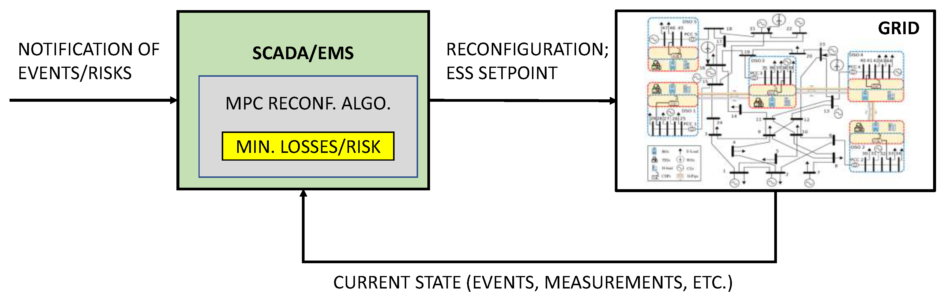
Figure 2.
16-bus distribution network [2]. During simulations, all branches were considered configurable.
Figure 2.
16-bus distribution network [2]. During simulations, all branches were considered configurable.

Figure 3.
Power generation from the distributed energy resources throughout a day. Maximum peak of 750 kW.
Figure 3.
Power generation from the distributed energy resources throughout a day. Maximum peak of 750 kW.

Figure 4.
Load variations throughout a day.
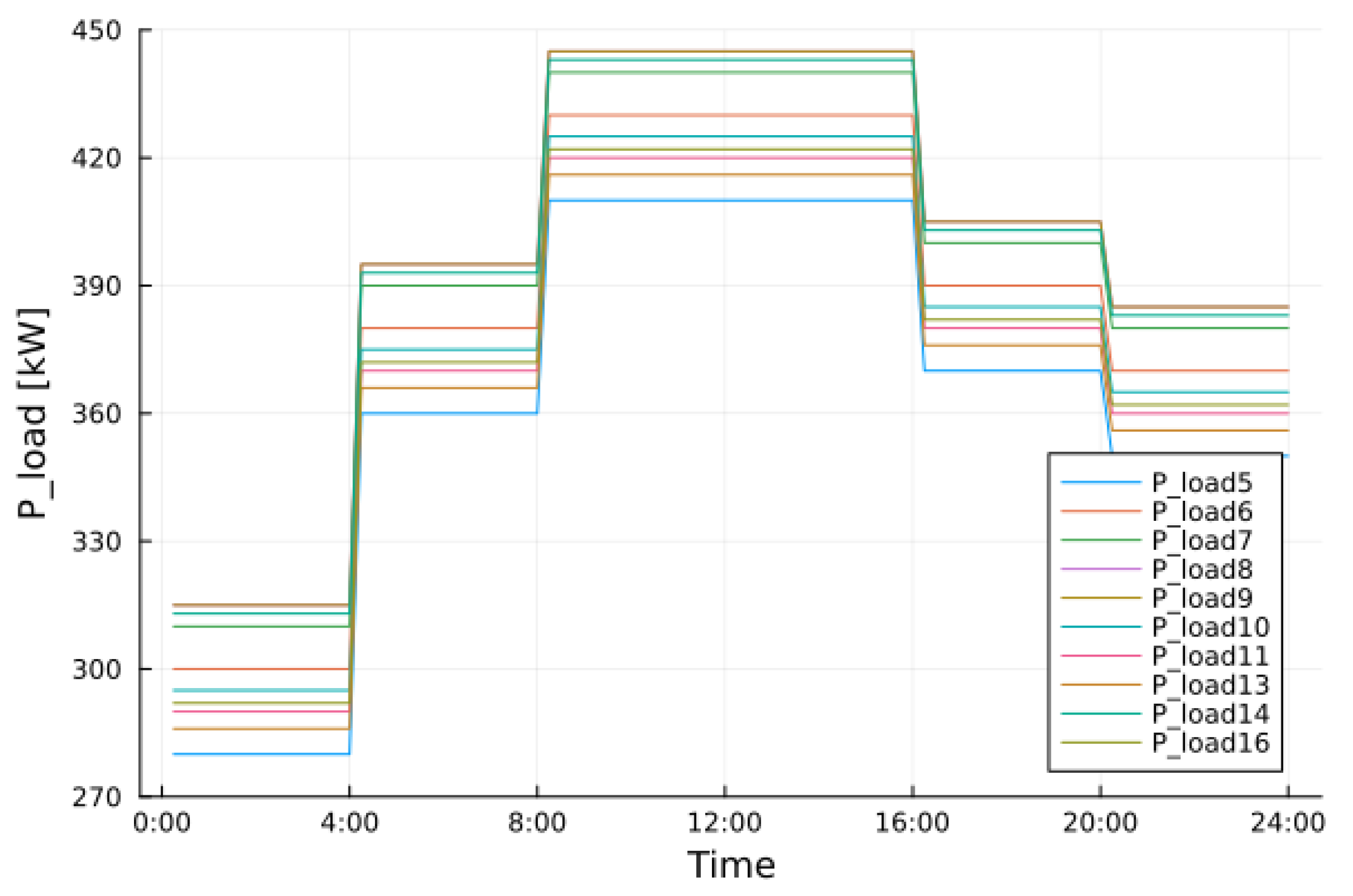
Figure 5.
Starting configuration with all opened branches. At the first iteration (namely 0:00), the topology is calculated.
Figure 5.
Starting configuration with all opened branches. At the first iteration (namely 0:00), the topology is calculated.

Figure 6.
Power flow in normal conditions. Each line represents , i.e., the power flow from bus i to bus j, with . For example, line 13 (L13) connects bus 9 (B9) and bus 11 (B11), and its power flow is .
Figure 6.
Power flow in normal conditions. Each line represents , i.e., the power flow from bus i to bus j, with . For example, line 13 (L13) connects bus 9 (B9) and bus 11 (B11), and its power flow is .

Figure 7.
Power flow of line 16 (L16) in normal conditions. The power flow is plotted considering the line from bus 15 (B15) to bus 16 (B16), i.e., , and vice versa ().
Figure 7.
Power flow of line 16 (L16) in normal conditions. The power flow is plotted considering the line from bus 15 (B15) to bus 16 (B16), i.e., , and vice versa ().
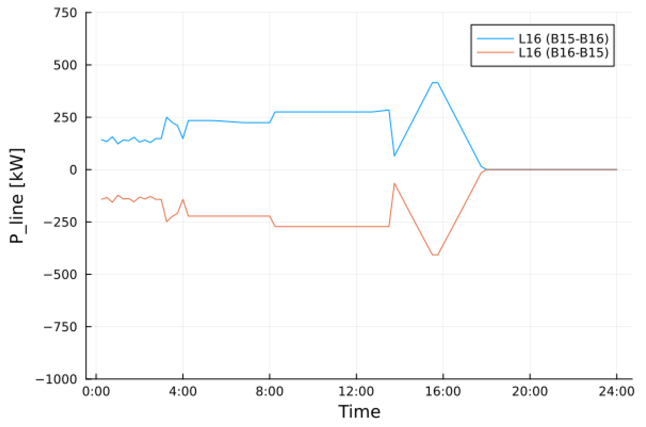
Figure 8.
ESS power in normal conditions. Lower bound at −1000 kW; maximum value of ≈220 kW reached by ESS 7.
Figure 8.
ESS power in normal conditions. Lower bound at −1000 kW; maximum value of ≈220 kW reached by ESS 7.
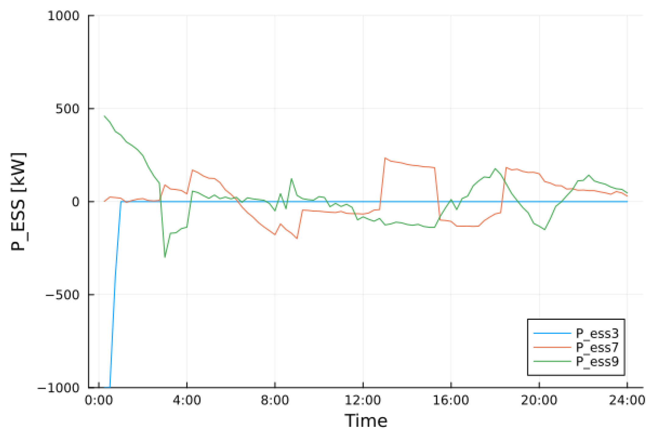
Figure 9.
ESS energy in normal conditions. Reference value is 80% of the maximum capacity, i.e., 1600 kWh.
Figure 9.
ESS energy in normal conditions. Reference value is 80% of the maximum capacity, i.e., 1600 kWh.

Figure 10.
Faults occur at 8:45 for L18, 14:45 for L11 and at 20:00 for L4 and L8. The island is formed at 20:00.
Figure 10.
Faults occur at 8:45 for L18, 14:45 for L11 and at 20:00 for L4 and L8. The island is formed at 20:00.

Figure 11.
ESSs power during the simulation of an adverse event. Vertical bars indicate line faults.
Figure 11.
ESSs power during the simulation of an adverse event. Vertical bars indicate line faults.
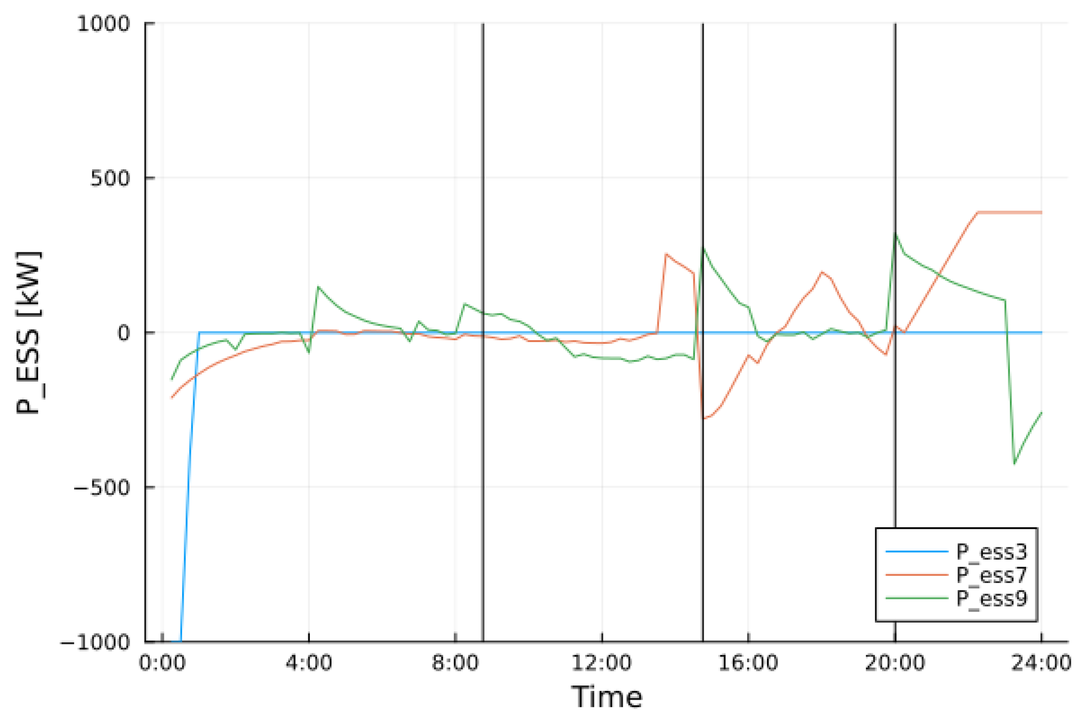
Figure 12.
ESSs energy during the simulation of an adverse event. Vertical bars indicate line faults. Reference value is 80% of the maximum capacity, i.e., 1600 kWh.
Figure 12.
ESSs energy during the simulation of an adverse event. Vertical bars indicate line faults. Reference value is 80% of the maximum capacity, i.e., 1600 kWh.
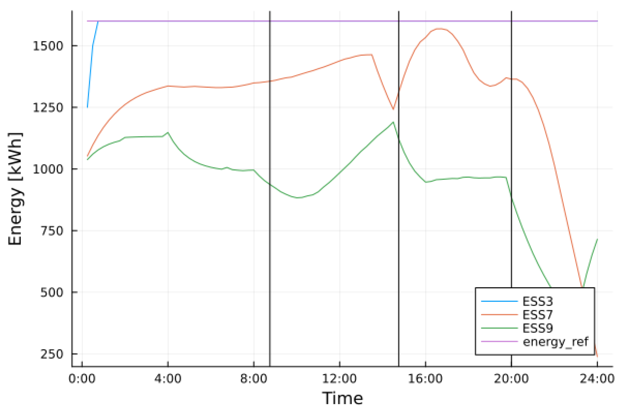
Figure 13.
Power flow of line L16 in fault conditions. The power is plotted considering the line from bus 15 to bus 16 and vice versa. The power flow is zero when the line is disconnected due the reconfiguration that occurs from 14:45 to just before 20:00.
Figure 13.
Power flow of line L16 in fault conditions. The power is plotted considering the line from bus 15 to bus 16 and vice versa. The power flow is zero when the line is disconnected due the reconfiguration that occurs from 14:45 to just before 20:00.
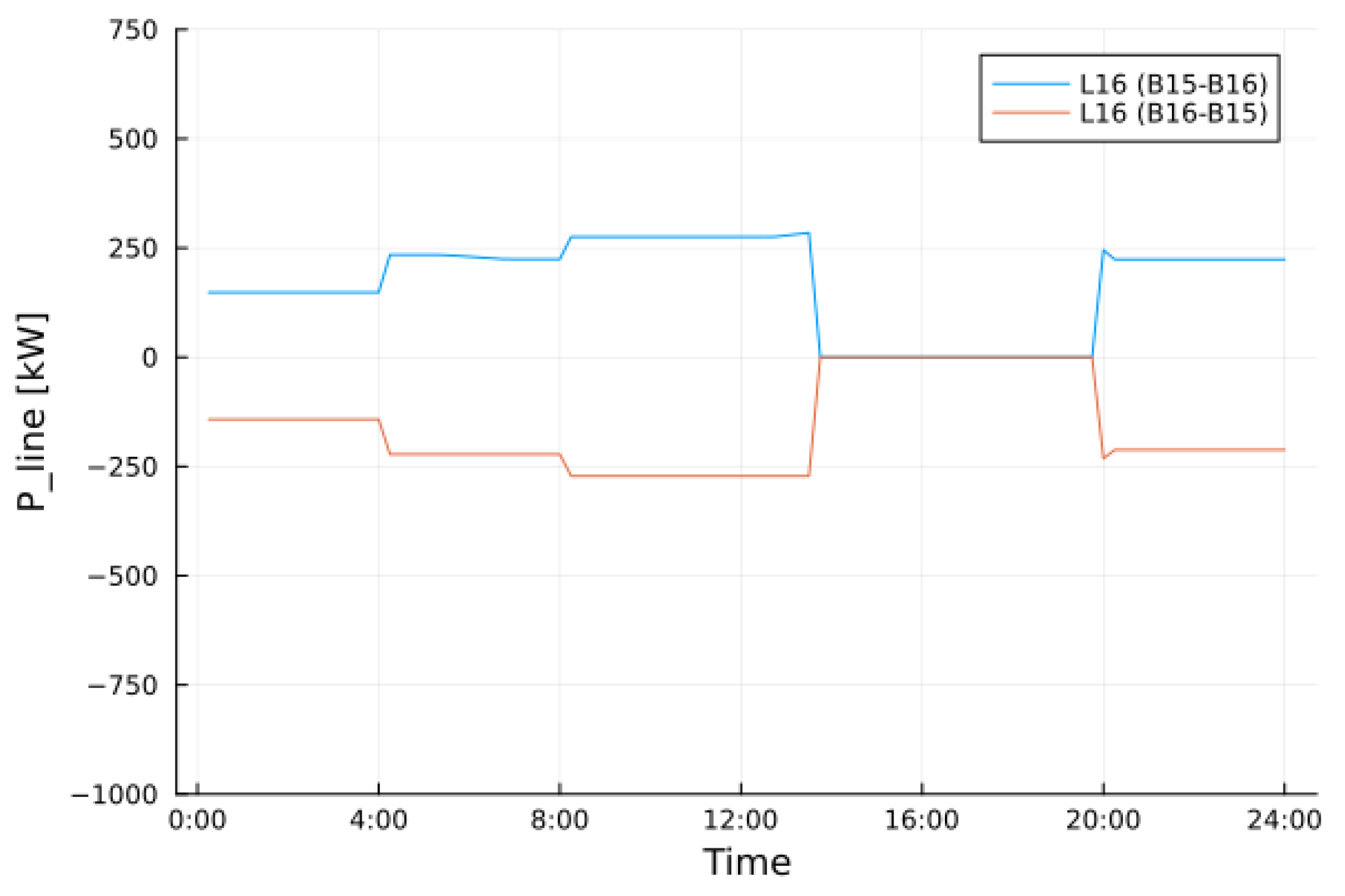
Figure 14.
Power flow of all lines in fault conditions. Each line represents , i.e., the power flow from bus i to bus j, with . For example, line 13 (L13) connects bus 9 (B9) and bus 11 (B11).
Figure 14.
Power flow of all lines in fault conditions. Each line represents , i.e., the power flow from bus i to bus j, with . For example, line 13 (L13) connects bus 9 (B9) and bus 11 (B11).

Figure 15.
Losses in static scenario.

Figure 16.
Ratio of losses/total power absorbed in static scenario. The total mean loss is 4.9%.
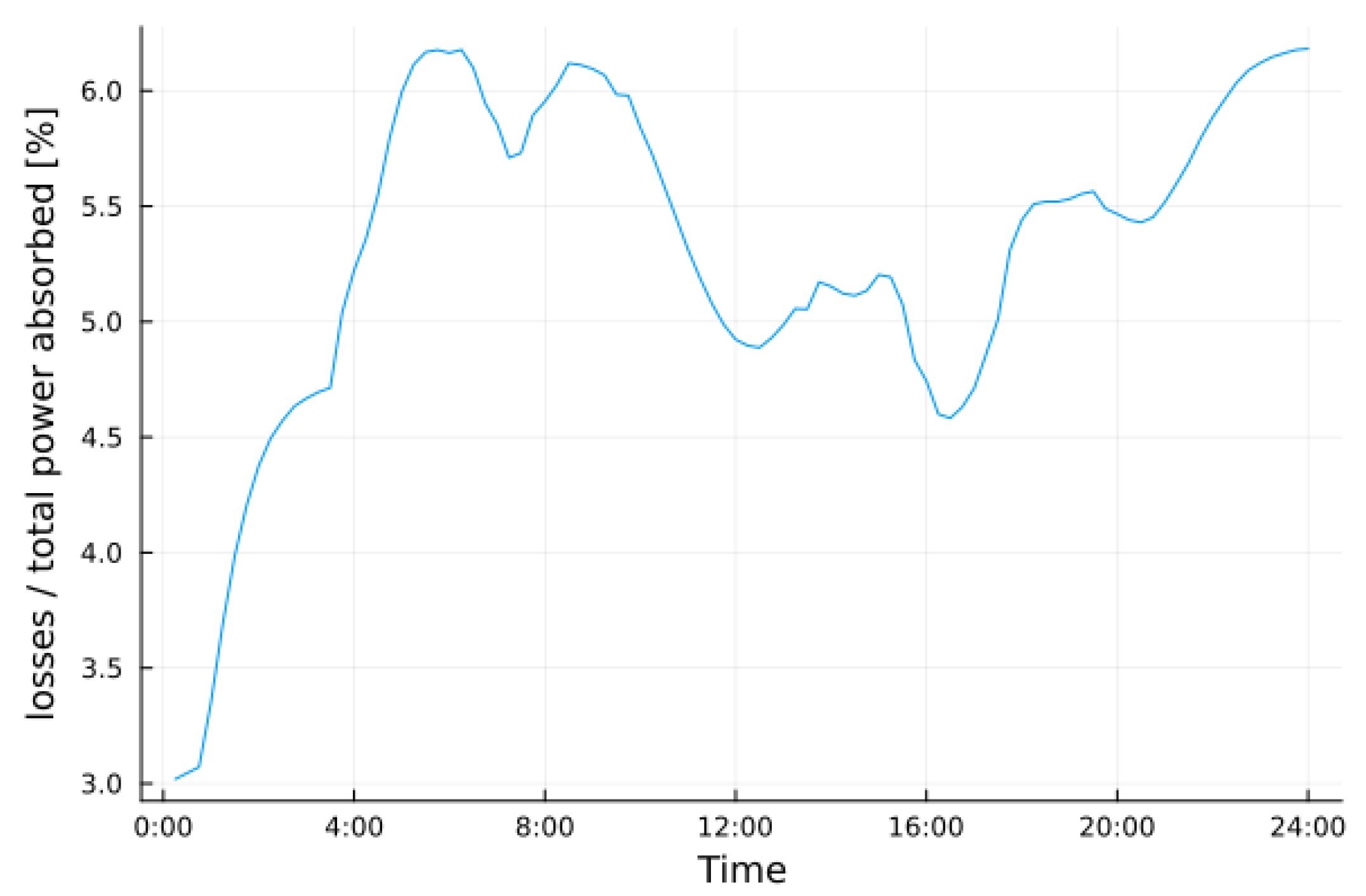
Figure 17.
Losses in the normal conditions scenario.

Figure 18.
Ratio of losses/total power absorbed in normal conditions scenario. The total mean loss is 4.6%.
Figure 18.
Ratio of losses/total power absorbed in normal conditions scenario. The total mean loss is 4.6%.

Figure 19.
Losses in the adverse events scenario.
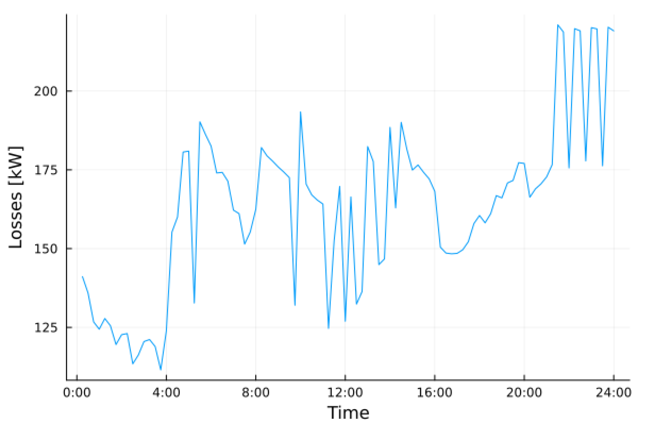
Figure 20.
Ratio of losses/total power absorbed in adverse events scenario. The total mean loss is 5.01%.
Figure 20.
Ratio of losses/total power absorbed in adverse events scenario. The total mean loss is 5.01%.

Figure 21.
Time elapsed under normal conditions.
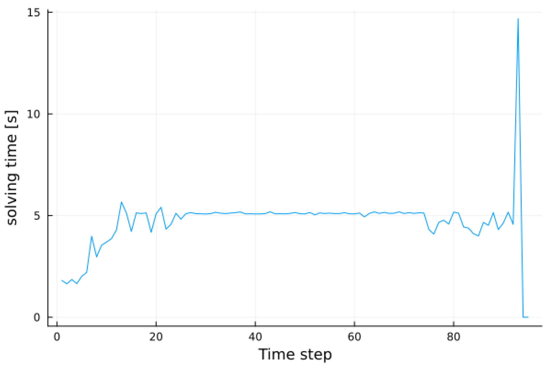
Figure 22.
Time elapsed under in fault conditions.


Table 1.
Summary of reviewed articles.
| Ref. | Control Problem and Objectives | Methodology | Dynamic | Islanding |
|---|---|---|---|---|
| [2] | Loss reduction and resilience increase in medium-voltage electricity grids | Economic MPC | No | No |
| [4] | Minimization of active energy losses and oswitching manipulation costs | DRL (Deep Q-Network) | Yes | No |
| [5] | Minimization of operational costs and differences with already-adopted strategies | Batch-constrained RL (Soft Actor-Critic) | Yes | No |
| [6] | Minimization of network losses and operational costs | DRL (Deep Q-Network) | Yes | No |
| [7] | Minimization of network losses | DRL (Deep Q- Learning, Dueling Deep Q-Learning, Deep Q-Learning with prioritized experience replay, Soft Actor-Critic, Proximal Policy Optimization) | No | No |
| [8] | Voltage Control in Active Distribution Networks | Safe DRL (Deep Deterministic Policy Gradient Algorithm) | No | No |
| [9] | Minimization of daily operation costs | Stochastic MPC | Yes | No |
| [10] | Minimization of operation costs | Stochastic MPC | Yes | No |
| [11] | Minimization of daily operation costs | Stochastic MPC | Yes | No |
| [12] | Maximization of energy savings and thermal comfort | MPC | Yes | No |
| [13] | Tracking operating points’ changes and maximization of network structural flexibility and error-tolerance | Distributed MPC | Yes | No |
| [14] | Minimization of system costs and stabilization after topology changes | Distributed MPC | Yes | No |
| [17] | Minimization of line losses | Linear Programming | No | No |
| [18] | Minimization of system’s active power losses | Genetic Algorithm and Mixed-Integer Linear Programming | No | No |
| [19] | Minimization of the total active power injected in the network by a given set of substations | Mixed-Integer Quadratically Constrained Programming | No | No |
| [21] | Maximization of restored active loads during faults | Mixed-Integer Linear Programming | No | Yes |
| Present paper | Minimization of losses; reaction to adverse events | MPC | Yes | Yes |
Table 2.
Nomenclature used in the paper.
| Symbol | Explanation |
|---|---|
| Status of the switch at line ( if line is connected, zero otherwise). | |
| Series susceptance in the -model of line . | |
| Weights in the objective function. | |
| Voltage phase angle at bus i. | |
| Difference between the phase angle at bus j and the phase angle at bus i. | |
| Set of links in the electricity grid. | |
| Objective function. | |
| Graph modelling the electricity grid. | |
| Series conductance in the -model of line . | |
| h | Time index. |
| Bus indices. | |
| k | Current time. |
| N | MPC control horizon. |
| Set of buses directly connected to bus i. | |
| Active and reactive power injection into the grid at bus i. | |
| Active and reactive power flowing from bus i to bus j. | |
| Power generated by the generator at substation SB. | |
| Power load demand. | |
| ESS capacity [kWh] at bus i. | |
| , | Active/reactive power of the ESS at bus i. |
| Auxiliary variable. | |
| Subset of . | |
| SOC of the ESS at bus i. | |
| Reference SOC level of the ESS at bus i. | |
| Auxiliary variable. | |
| T | MPC sampling time. |
| Auxiliary variable. | |
| Auxiliary variable. | |
| Set of buses in the electricity grid. | |
| Voltage level at bus i. |
Table 3.
Bus types.
| Bus Types | Bus Numbers |
|---|---|
| Substations | 1, 2, 3. |
| Hosting ESS | 3, 7, 9. |
| Loads buses | 5, 6, 7, 8, 9, 10, 11, 13, 14, 16. |
| Hosting DG | 4, 12, 15. |
Table 4.
Conductance and susceptance in per-unit notation.
| Link | G | B |
|---|---|---|
| L1 | 0.225 | 0.3 |
| L5 | 0.24 | 0.33 |
| L4 | 0.27 | 0.54 |
| L7 | 0.12 | 0.12 |
| L2 | 0.33 | 0.33 |
| L9 | 0.24 | 0.33 |
| L10 | 0.33 | 0.33 |
| L13 | 0.33 | 0.33 |
| L11 | 0.24 | 0.33 |
| L3 | 0.33 | 0.33 |
| L15 | 0.27 | 0.36 |
| L14 | 0.24 | 0.33 |
| L16 | 0.24 | 0.33 |
| L6 | 0.12 | 0.12 |
| L12 | 0.12 | 0.12 |
| L8 | 0.27 | 0.36 |
| L17 | 0.12 | 0.12 |
| L18 | 0.12 | 0.12 |
| L19 | 0.12 | 0.12 |
| L20 | 0.27 | 0.36 |
Table 5.
Lines Fault.
| Fault Time | Line |
|---|---|
| 8:45 | L18 |
| 14:45 | L11 |
| 20:00 | L4 and L8 |
Disclaimer/Publisher’s Note: The statements, opinions and data contained in all publications are solely those of the individual author(s) and contributor(s) and not of MDPI and/or the editor(s). MDPI and/or the editor(s) disclaim responsibility for any injury to people or property resulting from any ideas, methods, instructions or products referred to in the content. |
© 2023 by the authors. Licensee MDPI, Basel, Switzerland. This article is an open access article distributed under the terms and conditions of the Creative Commons Attribution (CC BY) license (https://creativecommons.org/licenses/by/4.0/).
Share and Cite
MDPI and ACS Style
Donsante, M.; Tortorelli, A.; Di Giorgio, A.; Liberati, F. A Model Predictive Control Algorithm for the Reconfiguration of Radially Operated Grids with Islands. Electronics 2023, 12, 4982. https://doi.org/10.3390/electronics12244982
AMA Style
Donsante M, Tortorelli A, Di Giorgio A, Liberati F. A Model Predictive Control Algorithm for the Reconfiguration of Radially Operated Grids with Islands. Electronics. 2023; 12(24):4982. https://doi.org/10.3390/electronics12244982
Chicago/Turabian StyleDonsante, Manuel, Andrea Tortorelli, Alessandro Di Giorgio, and Francesco Liberati. 2023. "A Model Predictive Control Algorithm for the Reconfiguration of Radially Operated Grids with Islands" Electronics 12, no. 24: 4982. https://doi.org/10.3390/electronics12244982
Note that from the first issue of 2016, this journal uses article numbers instead of page numbers. See further details here.