
Enhanced Control of Back-to-Back Converters in Wind Energy Conversion Systems Using Two-Degree-of-Freedom (2DOF) PI Controllers

Department of Electrical Engineering, College of Engineering and Petroleum, Kuwait University, P.O. Box 5969, Safat, Kuwait City 13060, Kuwait
Electronics 2023, 12(20), 4221; https://doi.org/10.3390/electronics12204221
Submission received: 16 September 2023
/
Revised: 10 October 2023
/
Accepted: 10 October 2023
/
Published: 12 October 2023
(This article belongs to the Special Issue Power Electronics for Renewable Energy Systems: Latest Advances and Prospects)
Abstract
:The performance of a full-scale wind energy conversion system is dependent on the control system of the back-to-back power electronics converter. Different controllers have been proposed in the literature, many of which are variations of a generalized two-degrees-of-freedom (2DOF) PI controller. This paper presents a design method for the parameters of a 2DOF PI controller for the stator current, generator speed, grid current, and DC bus voltage control. The controller can be designed using a general independent zero and pole placement method. The proposed and conventional methods are analyzed based on their ability to track references, reject disturbances, and their sensitivity to noise. A tuning approach is proposed to enhance the controller’s bandwidth without sacrificing noise sensitivity or disturbance rejection capability. The conventional methods are shown to be special versions of the proposed design. Simulation results demonstrate the effectiveness of the proposed design.
1. Introduction
Wind power is a crucial renewable energy source with a low carbon footprint. The industry is expected to grow significantly in the coming decades. The Global Wind Energy Council (GWEC) projects that the total installed wind capacity will reach a milestone of 1 TW this year (2023), while the next TW is expected by 2030 [1]. In 2022, the total global capacity for wind energy exceeded 906 GW, with the share of offshore installations increasing to 7% [1]. Wind energy is expected to account for 36% of the total power generation by 2050 [2]. Various configurations are available to convert the mechanical energy of the wind turbine’s shaft into electrical energy that can be fed to the grid [3]. These configurations can be classified into five types [4]. Type 1 is a fixed-speed system that uses a squirrel cage induction generator connected to the grid through a soft starter. Type 2 allows for variable-speed operation by changing the rotor resistance of a wound-rotor induction generator. The variable speed operation increases the energy output of the wind turbine and also increases its life span. The main drawbacks of Type 2 are the limited range of variable speed operation, usually ±10%, and the losses caused by increasing the rotor resistance. Type 3 offers a wider speed range, usually ±30%, which improves energy production at various wind speeds. It is based on a doubly fed induction generator where the stator windings are directly connected to the grid while the rotor windings are connected to the grid through a partial scale power converter (usually rated for 30% of the total power). Type 4 allows for a full variable speed range and uses a synchronous generator connected to the grid through a full-scale power converter. In Type 5, the synchronous generator is connected directly to the grid, and a variable ratio transmission is used to achieve the variable speed operation. The partial scale (Type 3) and the full-scale (Type 4) are the two most advanced and commonly implemented technologies today, with this paper focusing on Type 4. However, the method proposed in this paper can also be applied to Type 3.
Power electronics converters are necessary for these systems to convert the generator’s variable voltage and variable frequency into the appropriate voltage and frequency for the grid [5]. The back-to-back converter is a commonly used full-scale power converter consisting of a machine-side converter (AC-DC) and a grid-side converter (DC-AC) linked through a DC bus. IGBT or SiC switches could be used in the converter, with the latter showing advantages in efficiency, cost, and volume [6]. The converter’s control system is an integral part of the system, with the machine-side converter controlling the generator’s current and speed for maximum wind power extraction and the grid-side converter controlling the DC bus voltage and the injected power to the grid [7].
Usually, a cascaded control structure consisting of an inner loop inside an outer control loop is implemented for both converters. For the machine-side converter, the inner loop controls the stator currents and, thus, the electromagnetic torque, while the outer loop controls the rotational speed of the generator. The inner loop controls the grid currents on the grid-side converter based on the desired real or reactive power injected into the grid. An outer loop can be used to control the DC bus voltage. In general, four controllers are required: the stator current controller, the generator speed controller, the grid current controller, and the DC bus voltage controller.
Many techniques have been proposed to improve the effectiveness of the conventional PI controller. For the current controllers, these techniques include: (1) Designing with pole-zero cancellation along with state feedback decoupling control, with or without active damping [8], (2) Implementing Internal Model Control (IMC) [9], and (3) Using a Complex Vector Current Controller [10,11]. All of these methods can be generalized as a two-degrees-of-freedom (2DOF) PI controller [12]. The robustness of the 2DOF PI current controller is analyzed in [13]. In [14], a tuning approach of 2DOF PI controllers is proposed for the current controller. The proposed approach improves the disturbance rejection while slightly sacrificing the reference-tracking capability of the controller. A current controller that combines a two-degrees-of-freedom internal model control with active damping is proposed in [15]. In [16], a direct discrete-time current regulator is proposed based on the flux model for salient pole machines. A discrete PI controller with a deadbeat response control structure is proposed in [17]. Additionally, [18] proposed an online parameter estimation for the current controller, while [19] utilized a combined resonant and 2DOF controller to suppress current harmonics. If a first-order L filter is used to interface the grid-side converter to the grid, the same techniques could be applied to the grid current control. The 2DOF could also be utilized in the speed control loop [20,21]. In [22], a digital speed control system with an active damping structure is proposed. A composite variable structure PI controller is proposed in [23] for sensorless speed control. An adaptive neural network controller is presented in [24] for a system with a long shaft. An enhanced linear active disturbance rejection control method is proposed in [25]. The DC bus voltage could be controlled using various techniques.
The main contribution of this paper is proposing an enhanced way to control the back-to-back converters in wind energy conversion systems. The proposed control method, based on the two-degrees-of-freedom 2DOF PI controller, is applied to control the generator’s speed, the dq stator currents, the dc bus voltage, and the dq grid currents. Moreover, a tuning approach is proposed for all four controllers. Compared to [14], the proposed approach in this paper improves the controller’s bandwidth without sacrificing noise sensitivity or disturbance rejection capability. Moreover, the proposed approach can be applied to any of the four controllers in a wind energy conversion system. Compared to the conventional 2DOF PI, the proposed design is more general and allows for more freedom since it does not depend on pole-zero cancellation. The rest of this paper is organized as follows: the wind energy conversion system model is presented in Section 2. Section 3 discusses the design of the conventional PI and two-degrees-of-freedom (2DOF) PI controllers. Section 4 proposes the two-degrees-of-freedom (2DOF) PI controller. The proposed controller is simulated and compared to the conventional controllers in Section 5.
2. Model of Wind Energy Conversion System
Figure 1 shows the overall grid-interfaced, variable-speed wind turbine system and its control system. The three-bladed, horizontal-axis wind turbine (HAWT) is connected directly to the shaft of the permanent magnet synchronous generator (PMSG). The generator is connected to the grid through a full-scale, back-to-back AC-DC-AC converter, including a machine-side converter, a DC link, a grid-side converter, and a filter. The DC link provides the decoupling between the generator voltage and the grid voltage. The gating signals of the machine-side converter are used to turn the power electronics switches on or off in the converter to achieve the desired generator voltage set by the controller.
The machine-side converter is used to control the speed of the wind turbine for maximum wind power extraction. A cascaded control system is implemented with an outer speed loop and an inner current/torque loop. A maximum power point tracking (MPPT) algorithm is used to generate the speed command for the wind turbine. A two-degrees-of-freedom (2DOF) speed controller generates the current command based on the reference speed and actual speed obtained from measurements. A 2DOF current controller in the rotating reference frame generates the voltage command based on the reference currents and actual stator current obtained from the current sensors. Space vector pulse width modulation (SVPWM) generates the gating signals from the command voltages. The grid-side converter controls the DC link voltage and the reactive power injected into the grid. Again, a cascaded control system is implemented with an outer voltage and inner current loop. A two-degrees-of-freedom (2DOF) DC link controller generates the current command based on the desired DC link voltage and actual DC link voltage. A phase-locked-loop (PLL) is used to extract the phase angle of the grid. A 2DOF current controller in a reference frame rotating with the grid angle generates the voltage command based on the reference currents and actual grid currents obtained from the current sensors. Space vector pulse width modulation (SVPWM) generates the gating signals for the grid-side converter. This paper discusses the implementation of 2DOF PI controllers for the four controllers in Figure 1: the speed controller, stator current controller, DC link voltage controller, and grid current controller. A new tuning method for the coefficient of the 2DOF PI controllers is proposed and verified using detailed simulation in the PLECS software ver. 4.7.
The electric model of the PMSG in the synchronous reference frame can be obtained by applying Park transformation with the rotor electric angle as follows [26]:
The electromagnetic torque and the mechanical model of the PMSG are as follows:
where is the stator resistance, is the stator direct-axis inductance, is the stator quadrature-axis inductance, P is the number of poles, J is the moment of inertia, B is the friction coefficient, is the electrical frequency, is the mechanical frequency, is the electromagnetic torque, and is the turbine mechanical torque.
The model of the grid and the filter in the dq reference frame rotating with the grid angle obtained using PLL is as follows [27]:
The DC bus voltage equation is given by
where is the equivalent resistance of the filter and the grid, is the equivalent inductance of the filter and the grid, and are the transformed three-phase grid voltages into the rotating reference frame, is the capacitance of the DC link, is the DC current flowing from the machine-side converter, and is the DC current flowing into the grid-side converter.
3. Conventional PI and Two-Degrees-of-Freedom (2DOF) PI Controllers
A two-degrees-of-freedom (2DOF) PI controller for a first-order plant is shown in Figure 2a:
The plant in Figure 2a can represent any of the systems shown in Figure 3. y is the output of the system, n is the noise in the measurement, u is the command input to the plant, and r is the desired reference that the output y should track. P(s) is a first-order transfer function representing the plant dynamics while d represents the disturbance. The controller’s three main coefficients are , , and . By estimating the disturbance d, a feedforward term is used to cancel the disturbance of the plant d. A limiter block is utilized to limit the command input u to the plant. Finally, to avoid the windup of the controller, anti-windup control is implemented with a coefficient .
The limiter and anti-windup could be neglected in order to analyze the system’s response at normal operating conditions, as shown in Figure 2b. Since only estimates the disturbance d, the term represents the difference between the estimated and actual disturbance. Table 1 summarizes the parameters a, b, and the disturbance d for the subsystems shown in Figure 3 and the controller shown in Figure 2.
In Figure 2a, if P(s) is a first-order transfer function given by
then the output y could be derived in terms of the reference r, the disturbance , and the noise n as
where G(s) is the reference-tracking transfer function, H(s) is the disturbance rejection transfer function, and T(s) is the noise sensitivity transfer function given by
The transfer functions have two poles and one zero. Defining z, , and as the absolute values of the left-half plane (LHP) zero and the two poles of G(s), respectively,
Based on the desired poles and zero of G(s), a pole-zero placement method could be used to design the controller coefficients as follows:
In this case, the reference tracking transfer function G(s), the disturbance rejection transfer function H(s), and the noise sensitivity transfer function T(s) are as follows:
where is the zero of the noise sensitivity transfer function T(s) given by
3.1. Design of the Conventional PI Controller
The conventional PI controller is a particular case of the 2DOF PI controller, which could be obtained by setting . In this case, the reference tracking transfer function G(s) will be identical to the noise sensitivity transfer function T(s), as shown in Equations (11) and (13).
For a desired reference tracking bandwidth α, one way to design the coefficients of a conventional PI controller is using pole-zero cancellation by choosing the poles and zero as follows:
The output y could be derived as
Note that G(s) and T(s) are identical as expected, and one pole defines the behavior of both transfer functions. Define M as the magnitude of the noise sensitivity transfer function T(s) at the switching frequency . Then, M could be obtained by evaluating of the magnitude of the transfer function T(s) when as follows:
Alternatively, if the damping term b is negligible, a pole-placement method could be used. If the poles are selected to be real and repeated , then the zero could be found using (23) as . Then, the reference tracking transfer function becomes
For a desired bandwidth α, p could be found by solving ,
3.2. Conventional Design of 2DOF PI Controller
The conventional 2DOF PI controller coefficients are usually selected based on pole-zero cancellation. The 2DOF PI controller could be represented in the active damping form [28]. In this case, the first pole is selected as in (24) while the second pole and the zero could be selected as
where is the active damping form appearing in the canceled pole and zero. Then, the controller’s coefficients are as follows:
In this case, the output y could be derived as
where is given by
This shows an improved disturbance rejection compared to the PI controller in (28) since one of the two poles of H(s) is moved further to the left. In both cases, pole-zero cancellation () was selected to achieve a first-order reference-tracking response in G(s). Again, the magnitude of the noise sensitivity transfer function at the switching frequency M depends on the two poles and only since
Using where T is given by (38), an approximated equation could be derived if and , which is usually the case as
This equation indicates that the noise sensitivity at the switching frequency M depends on the sum of the two poles . If the sum of the two poles is defined as
Then, Figure 4a shows that the relation between the main pole (bandwidth) and the canceled pole is approximately linear for a given M.
Now, another equation is required to choose and . Defining the center frequency of H(s) as
Figure 4b shows the relation between the center frequency of H(s) and the bandwidth of G(s) using pole-zero cancellation. The peak value of the center frequency occurs when the two poles are identical , as indicated by the red dot. Any point on the curve could be selected; however, values further to the left of the peak are not desirable since both the bandwidth α and center frequency are reduced, while values to the right result in disturbance rejection worse than the conventional PI controller. To maximize the disturbance rejection capability, the zero and poles will be selected based on pole-zero cancellation as follows:
Finally, for a desired bandwidth α, the controller coefficient is selected as in (17) while and coefficients are selected as
4. Proposed Two-Degrees-of-Freedom (2DOF) PI Controller
The proposed design does not depend on the pole-zero cancellation. To achieve the same disturbance rejection and noise sensitivity, the poles are selected as before to achieve the same disturbance rejection and noise sensitivity. In this case, the center frequency . Using the conventional 2DOF PI design, the bandwidth is . A desired bandwidth of is impossible with the pole-zero cancellation since it is not on the curve of Figure 4b. However, without pole-zero cancellation, we can choose the zero of G(s) to achieve the desired bandwidth α. For a desired bandwidth α, z could be found by solving , where G is given by (20) as
To have the same disturbance rejection transfer function H(s) and noise sensitivity transfer function T(s), the poles are selected as the conventional 2DOF PI (). However, the proposed method does not use zero-pole cancellation since the zero could be selected independently. Define m to be a parameter that relates the zero and the pole as
where . Then, for the reference-tracking transfer function G(s) given by (20), the poles are selected as and the zero is defined as in (46). The bandwidth α could be found by solving as,
The maximum percent overshoot could be found by deriving the time domain expression of the response for a step input using the inverse Laplace transform. In this case, the maximum percent overshoot is given by
Figure 5 shows the value of the zero, the bandwidth, and the maximum percent overshoot as a function of m. Selecting will result in the conventional PI controller, while the limit as represents the conventional 2DOF PI controller. The proposed design is more general since it allows for choosing any value for m between 2 and ∞. Values of m below 2 are undesirable since the overshoot is very high. The value of m could be selected based on the desired overshoot or bandwidth. Figure 5 shows three examples of selecting m based on a desired overshoot of , , and . Note that there is a trade-off between increasing the bandwidth and decreasing the overshoot, as seen in Figure 5b,c.
Alternatively, m could be selected based on the desired bandwidth. For instance, the desired bandwidth may be selected as two times the pole location 2p, which is double the bandwidth of the conventional 2DOF PI controller. In this case, substituting the bandwidth in (46) and (47), will result in the following zero:
and the maximum percent overshoot will be around 6.07% regardless of the system parameters a and b or the value of the bandwidth α. The controller coefficients are given by
In this case, the proposed controller can achieve double the bandwidth α for the same noise sensitivity as the conventional 2DOF PI controller.
5. Simulation Results and Discussion
The complete wind energy conversion system shown in Figure 6 was simulated in PLECS software ver. 4.7.
The mechanical torque of the wind turbine is modeled as a 2D lookup table as a function of the wind speed and the shaft speed . Table 2 summarizes the main system parameters.
The proposed 2DOF PI controller is compared to the conventional 2DOF PI controller and the conventional PI controller. To compare the controllers fairly, identical poles and are selected for the three controllers, resulting in exact disturbance rejection transfer function H(s) and noise sensitivity transfer function T(s). Table 3 shows the parameters of the proposed controller compared to the conventional PI and conventional 2DOF PI designs. The controller coefficients are selected using (17)–(19) based on the desired poles and zeros.
The bode amplitude plots of the reference-tracking transfer function G(s), the disturbance rejection transfer function H(s), and the noise sensitivity transfer function T(s) are shown in Figure 7. As expected, the disturbance rejection transfer function H(s) and noise sensitivity transfer function T(s) are identical for both the speed and DC bus voltage controller since the poles are identical.
The model shown in Figure 6 is simulated starting with a wind speed of 10 m/s and a reference DC bus voltage of 1200 V. Figure 8 shows the dynamic simulation results for the wind energy conversion system when the conventional PI controller is used to implement the speed controller, dq stator current controllers, DC bus voltage controller, and the dq grid current controllers.
A step change in the wind speed from 10 m/s to 9.5 m/s is introduced at t = 5 s, resulting in a change in the generator reference speed. To operate at the optimal power point, the generator speed in (rad/s) must be controlled to be
where R is the radius of the area swept by the turbine blades and is the optimal tip-speed ratio shown in Table 2. A step change in the reference DC bus voltage from 1200 V to 1100 V is introduced at t = 10 s to test the DC bus voltage controller. The same simulation is repeated for the conventional 2DOF PI controller and the proposed 2DOF PI controller, and the results are shown in Figure 9 and Figure 10, respectively.
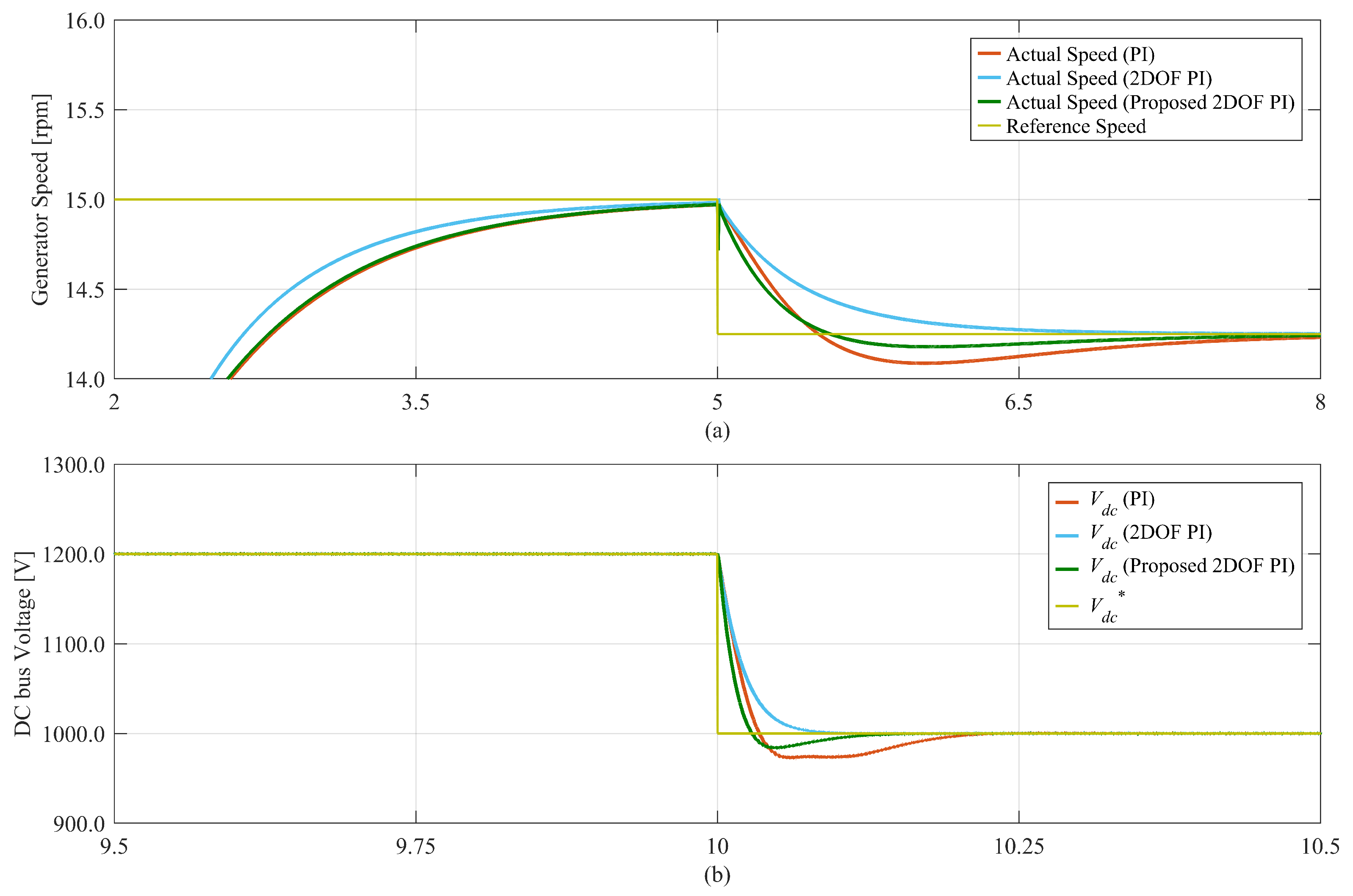
The simulation starts with an initial generator speed that is lower than the reference speed, as shown in Figure 10a. Therefore, the speed controller tries to generate a positive current command in order to generate an accelerating torque. However, the current command is limited to negative values to prevent PMSG from operating in motoring mode and absorbing current from the grid. For this reason, the acceleration is based on the mechanical torque from the wind. Around t = 2 s, as the error between the reference speed and the actual speed becomes smaller, a negative current command is generated, as shown in Figure 10c, indicating that power is being produced. At t = 5 s, as the wind speed changes, the generator reference speed also changes in order to operate at the optimal power production point. In order to reduce the generator speed to the new set point, more power is injected into the grid until the generator reaches a steady state operation at around t = 8 s. All controllers achieved the desired reference tracking; however, the dynamic response is not identical. The conventional and proposed 2DOF PI controllers show better current tracking compared to the PI controller. To ensure a fair comparison between the controllers, the speed and the DC bus voltage are compared in Figure 11 and Table 4.
The proposed controller was able to achieve higher bandwidth and thus reduce the rise time. The increase in the bandwidth came at the cost of a slight overshoot in the response. Compared to the PI controller, the overshoot was reduced significantly to 45% of the PI overshoot, while the bandwidth was reduced only to 80% of the PI bandwidth. Compared to the conventional 2DOF PI controller, the bandwidth was doubled while a 6% maximum percent overshoot was introduced. The simulated proposed design is just an example of a specific bandwidth. As shown in Section 4, changing the value of m will result in different bandwidths and overshoot. A trade-off exists between increasing the bandwidth and decreasing the overshoot, as shown in Figure 5.
6. Conclusions
This paper presents a novel approach to designing the 2DOF PI controllers for a full-scale wind energy conversion system. The method covers the design of controllers for stator currents, generator speed, grid currents, and the DC bus voltage. The controller design utilizes an independent zero and pole placement method, which can be tuned to increase bandwidth without compromising the disturbance rejection capabilities and the sensitivity to noise. The proposed design is a more generalized approach compared to the conventional PI controllers and the conventional 2DOF PI controller with pole-zero cancellation. In fact, it has been shown that both of these controllers can be considered as special versions of the proposed general design. The proposed design is more flexible and can be tuned to meet specific requirements. This study examines the trade-off between increasing bandwidth and decreasing the overshoot in the proposed method. Upon conducting a comparative analysis with the PI controller, it was observed that the overshoot was significantly reduced to 45% of the PI overshoot. However, the bandwidth only experienced a reduction to 80% of the PI bandwidth. Furthermore, in comparison to the conventional 2DOF PI controller, the bandwidth was noted to have doubled. Nevertheless, this advantage was achieved at the expense of introducing a maximum percentage overshoot of 6%. Simulation results confirm the effectiveness of the proposed design.
Funding
This project was “Partially” funded by Kuwait Foundation for the Advancements of Sciences under project code “PN18-15EE-02”.
Data Availability Statement
No new data were created or analyzed in this study. Data sharing is not applicable to this article.
Conflicts of Interest
The author declares no conflict of interest. The funders had no role in the design of the study, in the collection, analyses, or interpretation of data, in the writing of the manuscript, or in the decision to publish the results.
References
- Global Wind Energy Council. Global Wind Report 2023. Available online: https://gwec.net/globalwindreport2023/ (accessed on 12 September 2023).
- Bloomberg NEF (BNEF). New Energy Outlook 2022. Available online: https://about.bnef.com/new-energy-outlook/ (accessed on 12 September 2023).
- Hansen, A.D.; Iov, F.; Blaabjerg, F.; Hansen, L.H. Review of Contemporary Wind Turbine Concepts and Their Market Penetration. Wind Eng. 2004, 28, 247–263. [Google Scholar] [CrossRef]
- Yaramasu, V.; Wu, B.; Sen, P.C.; Kouro, S.; Narimani, M. High-power wind energy conversion systems: State-of-the-art and emerging technologies. Proc. IEEE 2015, 5, 740–788. [Google Scholar] [CrossRef]
- Blaabjerg, F.; Liserre, M.; Ma, K. Power electronics converters for wind turbine systems. IEEE Trans. Ind. Appl. 2012, 48, 708–719. [Google Scholar] [CrossRef]
- Loncarski, J.; Hussain, H.A.; Bellini, A. Efficiency, Cost, and Volume Comparison of SiC-Based and IGBT-Based Full-Scale Converter in PMSG Wind Turbine. Electronics 2023, 12, 385. [Google Scholar] [CrossRef]
- Blaabjerg, F.; Ma, K. Future on Power Electronics for Wind Turbine Systems. IEEE J. Emerg. Sel. Top. Power Electron. 2013, 1, 139–152. [Google Scholar] [CrossRef]
- Yepes, A.G.; Vidal, A.; Malvar, J.; López, O.; Doval-Gandoy, J. Tuning Method Aimed at Optimized Settling Time and Overshoot for Synchronous Proportional-Integral Current Control in Electric Machines. IEEE Trans. Power Electron. 2014, 29, 3041–3054. [Google Scholar] [CrossRef]
- Harnefors, L.; Nee, H.-P. Model-based current control of ac machines using the internal model control method. IEEE Trans. Ind. Appl. 1998, 34, 133–141. [Google Scholar] [CrossRef]
- Briz, F.; Degner, M.W.; Lorenz, R.D. Analysis and design of current regulators using complex vectors. IEEE Trans. Ind. Appl. 2000, 36, 817–825. [Google Scholar] [CrossRef]
- Zhao, L.; Song, W.; Ruan, Z. Discrete Domain Design Scheme of Complex-Vector Current Controller for Induction Motor at Low Switching Frequency. IEEE Trans. Transp. Electrif. 2023, 9, 404–415. [Google Scholar] [CrossRef]
- Hinkkanen, M.; Awan, H.A.A.; Qu, Z.; Tuovinen, T.; Briz, F. Current Control for Synchronous Motor Drives: Direct Discrete-Time Pole-Placement Design. IEEE Trans. Ind. Appl. 2016, 52, 1530–1541. [Google Scholar] [CrossRef]
- Hussain, H.A. Design and Robustness Analysis of 2DOF PI Synchronous-Frame Current Regulator for Salient PMSM Drives. In Proceedings of the Conference Record of the 2019 IEEE Energy Conversion Congress and Exposition (ECCE), Baltimore, MD, USA, 29 September–3 October 2019; pp. 6155–6160. [Google Scholar] [CrossRef]
- Hussain, H.A. Tuning and Performance Evaluation of 2DOF PI Current Controllers for PMSM Drives. IEEE Trans. Transp. Electrif. 2021, 7, 1401–1414. [Google Scholar] [CrossRef]
- Liang, W.; Liang, D.; Jia, S.; Chu, S.; Wang, H.; Zhang, H.; Liang, Y. Digital Current Controller Design for SPMSM With Low Switching-to-Fundamental Frequency Ratios. IEEE Trans. Ind. Appl. 2022, 58, 4685–4697. [Google Scholar] [CrossRef]
- Yuan, X.; Chen, J.; Jiang, C.; Lee, C.H.T. Discrete-Time Current Regulator for AC Machine Drives. IEEE Trans. Power Electron. 2022, 37, 5847–5858. [Google Scholar] [CrossRef]
- Wang, M.; Buticchi, G.; Li, J.; Gu, C.; Gerada, D.; Degano, M.; Xu, L.; Li, Y.; Zhang, H.; Gerada, C. 2-DOF Decoupled Discrete Current Control for AC Drives at Low Sampling-to-Fundamental Frequency Ratios. IEEE Trans. Transp. Electrif. 2023, 9, 2048–2058. [Google Scholar] [CrossRef]
- Kim, H.; Lorenz, R.D. Improved current regulators for IPM machine drives using on-line parameter estimation. In Proceedings of the Conference Record of the 2002 IEEE Industry Applications Conference. 37th IAS Annual Meeting (Cat. No.02CH37344), Pittsburgh, PA, USA, 13–18 October 2002; Volume 1, pp. 86–91. [Google Scholar] [CrossRef]
- Pan, Z.; Dong, F.; Zhao, J.; Wang, L.; Wang, H.; Feng, Y. Combined Resonant Controller and Two-Degree-of-Freedom PID Controller for PMSLM Current Harmonics Suppression. IEEE Trans. Ind. Electron. 2018, 65, 7558–7568. [Google Scholar] [CrossRef]
- Lin, S.; Cao, Y.; Wang, Z.; Yan, Y.; Shi, T.; Xia, C. Speed Controller Design for Electric Drives Based on Decoupling Two-Degree-of-Freedom Control Structure. IEEE Trans. Power Electron. 2023. [Google Scholar] [CrossRef]
- Harnefors, L.; Saarakkala, S.E.; Hinkkanen, M. Speed Control of Electrical Drives Using Classical Control Methods. IEEE Trans. Ind. Appl. 2013, 49, 889–898. [Google Scholar] [CrossRef]
- Yuan, X.; Chen, J.; Liu, W.; Lee, C.H.T. A Linear Control Approach to Design Digital Speed Control System for PMSMs. IEEE Trans. Power Electron. 2022, 37, 8596–8610. [Google Scholar] [CrossRef]
- Feng, W.; Bai, J.; Zhang, Z.; Zhang, J. A Composite Variable Structure PI Controller for Sensorless Speed Control Systems of IPMSM. Energies 2022, 15, 8292. [Google Scholar] [CrossRef]
- Malarczyk, M.; Zychlewicz, M.; Stanislawski, R.; Kaminski, M. Low-Cost Implementation of an Adaptive Neural Network Controller for a Drive with an Elastic Shaft. Signals 2023, 4, 56–72. [Google Scholar] [CrossRef]
- Wang, C.; Yan, J.; Heng, P.; Shan, L.; Zhou, X. Enhanced LADRC for Permanent Magnet Synchronous Motor With Compensation Function Observer. IEEE J. Emerg. Sel. Top. Power Electron. 2023, 11, 3424–3434. [Google Scholar] [CrossRef]
- Lipo, T.A. Analysis of Synchronous Machines, 2nd ed.; CRC Press: Boca Raton, FL, USA, 2012. [Google Scholar]
- Alcalá, J.; Bárcenas, E.; Cárdenas, V. Practical methods for tuning PI controllers in the DC-link voltage loop in Back-to-Back power converters. In Proceedings of the 12th IEEE International Power Electronics Congress, San Luis Potosi, Mexico, 22–25 August 2010; pp. 46–52. [Google Scholar] [CrossRef]
- Sul, S.-K. Design of Regulators for Electric Machines and Power Converters. In Control of Electric Machine Drive Systems; IEEE: Piscataway Township, NJ, USA, 2011; pp. 154–229. [Google Scholar] [CrossRef]
Figure 1.
Block diagram of the grid-interfaced, full-scale, variable-speed wind turbine system.
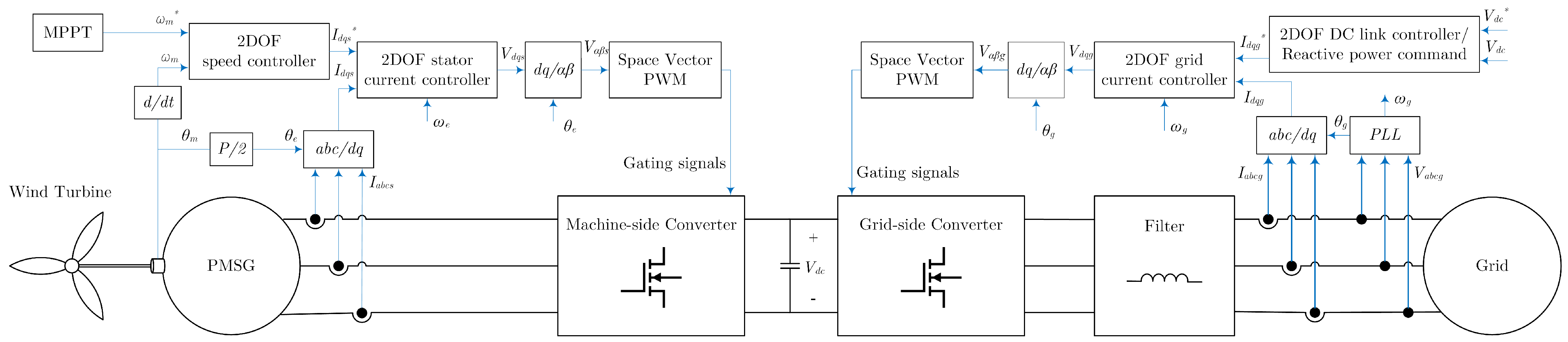
Figure 2.
Block diagram of the two-degrees-of-freedom PI controller (a) complete controller with the plant (b) neglecting the saturation.
Figure 2.
Block diagram of the two-degrees-of-freedom PI controller (a) complete controller with the plant (b) neglecting the saturation.
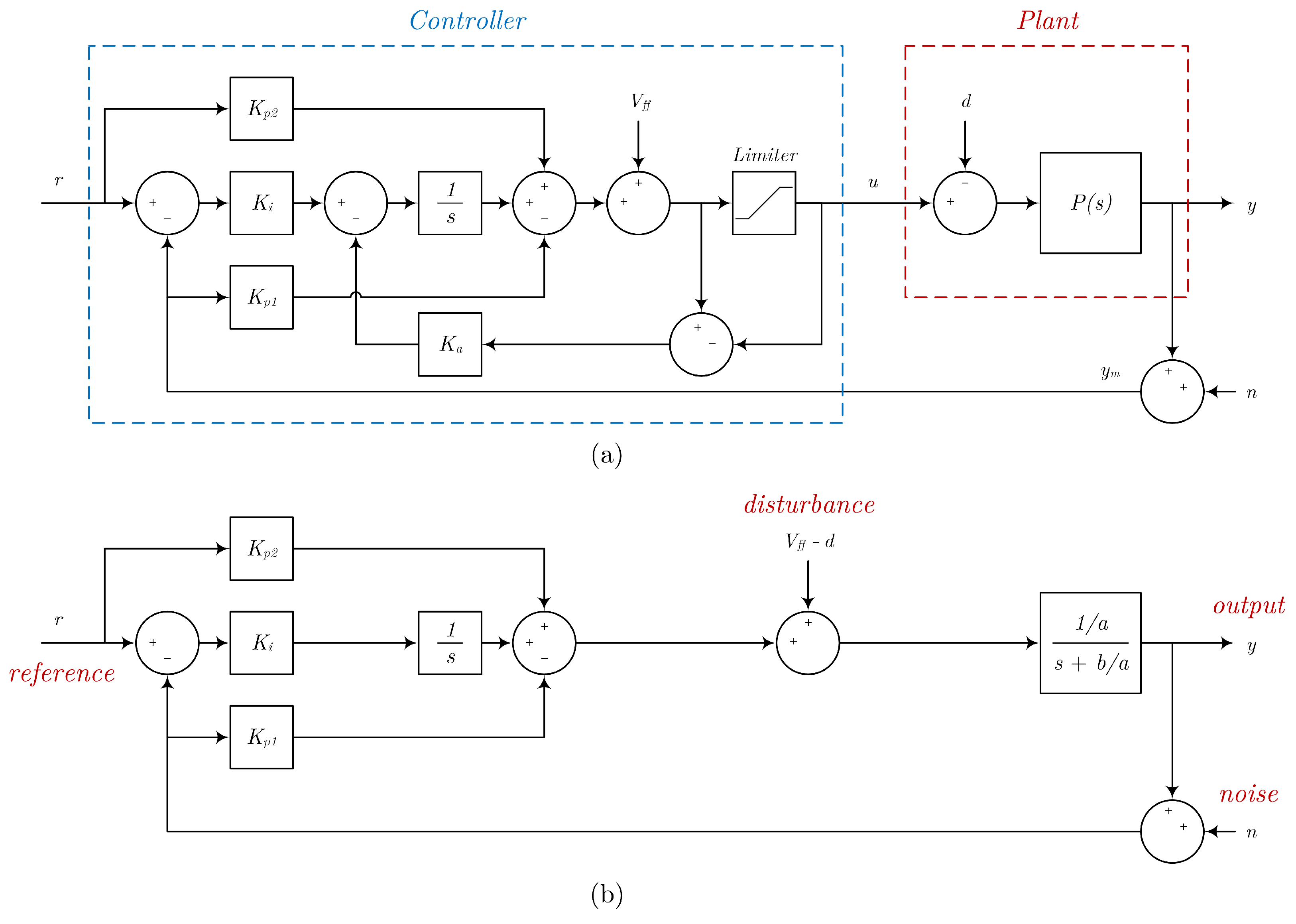
Figure 3.
Block diagrams of the models of the subsystems in the wind energy conversion system (a), stator d-axis and q-axis models (b), mechanical model (c), grid d-axis and q-axis models (c), dc link model (d).
Figure 3.
Block diagrams of the models of the subsystems in the wind energy conversion system (a), stator d-axis and q-axis models (b), mechanical model (c), grid d-axis and q-axis models (c), dc link model (d).

Figure 4.
(a) The canceled pole as a function of the bandwidth. (b) The center frequency as a function of the bandwidth where the red dot indicates the peak value of the center frequency.
Figure 4.
(a) The canceled pole as a function of the bandwidth. (b) The center frequency as a function of the bandwidth where the red dot indicates the peak value of the center frequency.
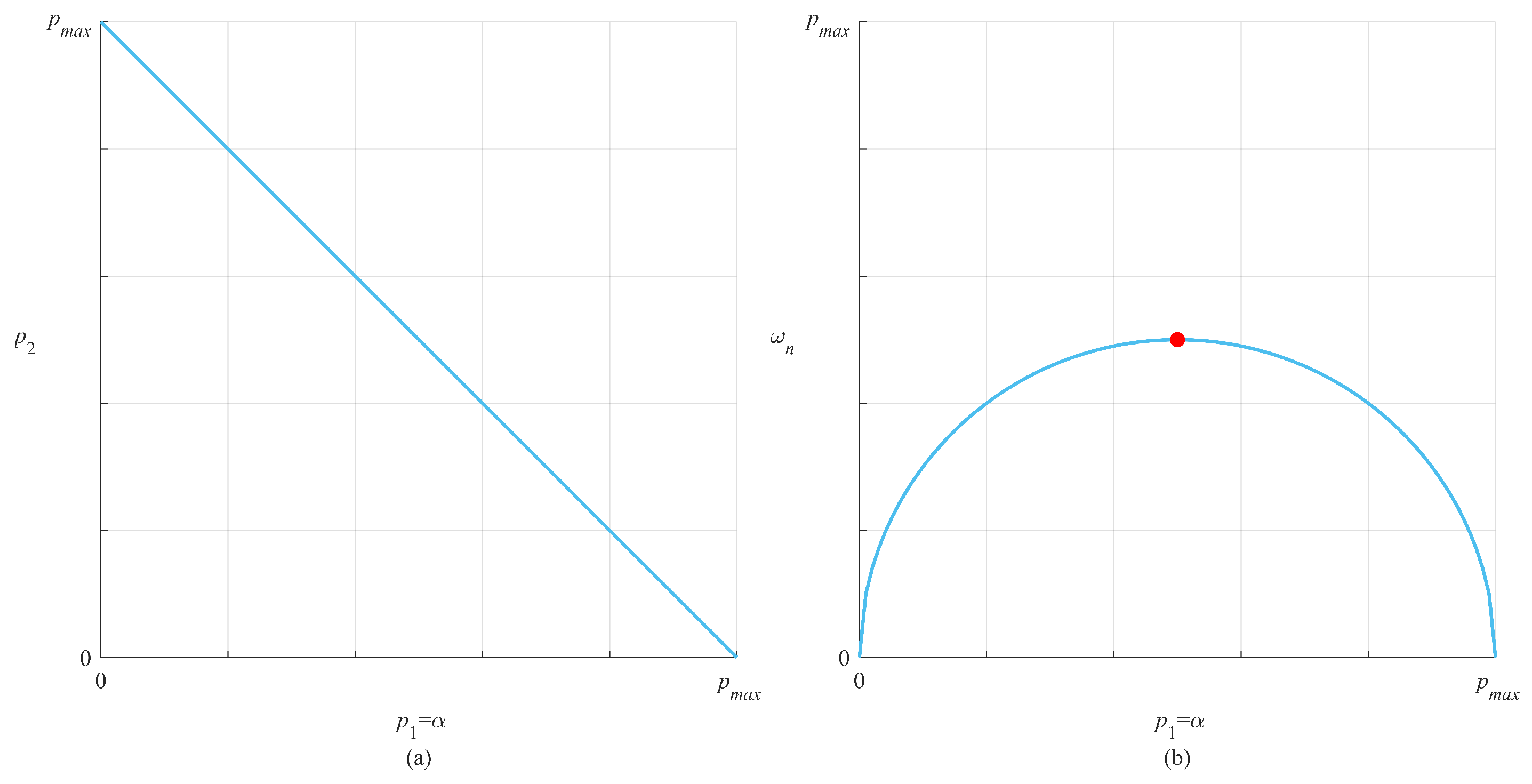
Figure 5.
(a) The ratio between the zero and pole p, (b) the maximum percent overshoot, (c) the ratio between the bandwidth α and the pole p.
Figure 5.
(a) The ratio between the zero and pole p, (b) the maximum percent overshoot, (c) the ratio between the bandwidth α and the pole p.
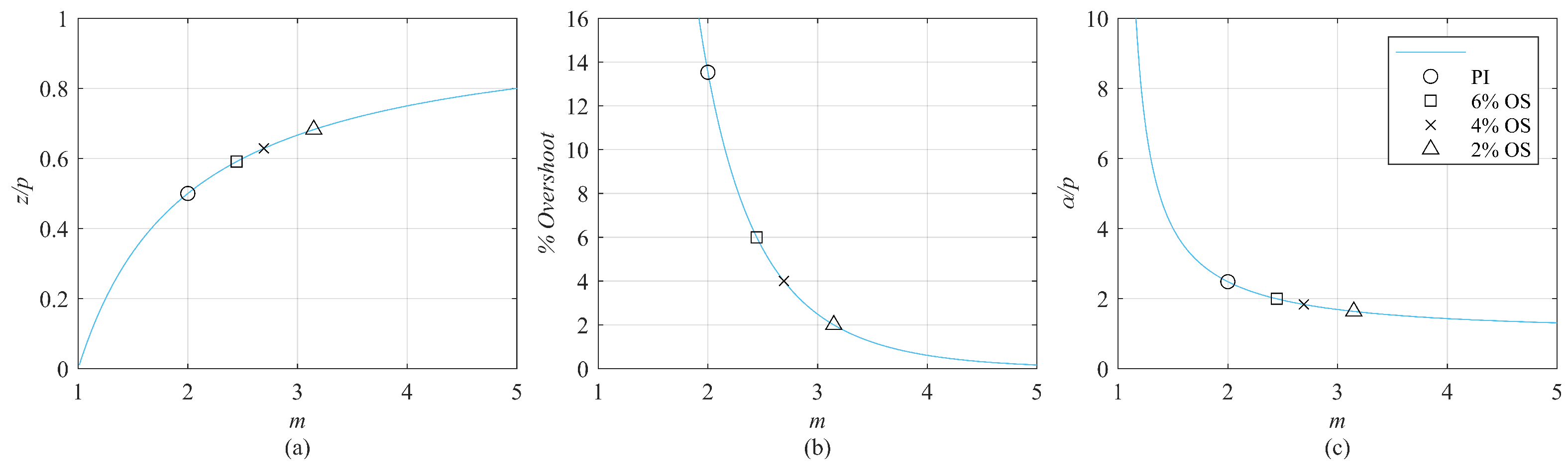
Figure 6.
PLECS model of the grid-interfaced, full-scale, variable-speed wind turbine system where the reference values are indicated using asterisks (*).
Figure 6.
PLECS model of the grid-interfaced, full-scale, variable-speed wind turbine system where the reference values are indicated using asterisks (*).
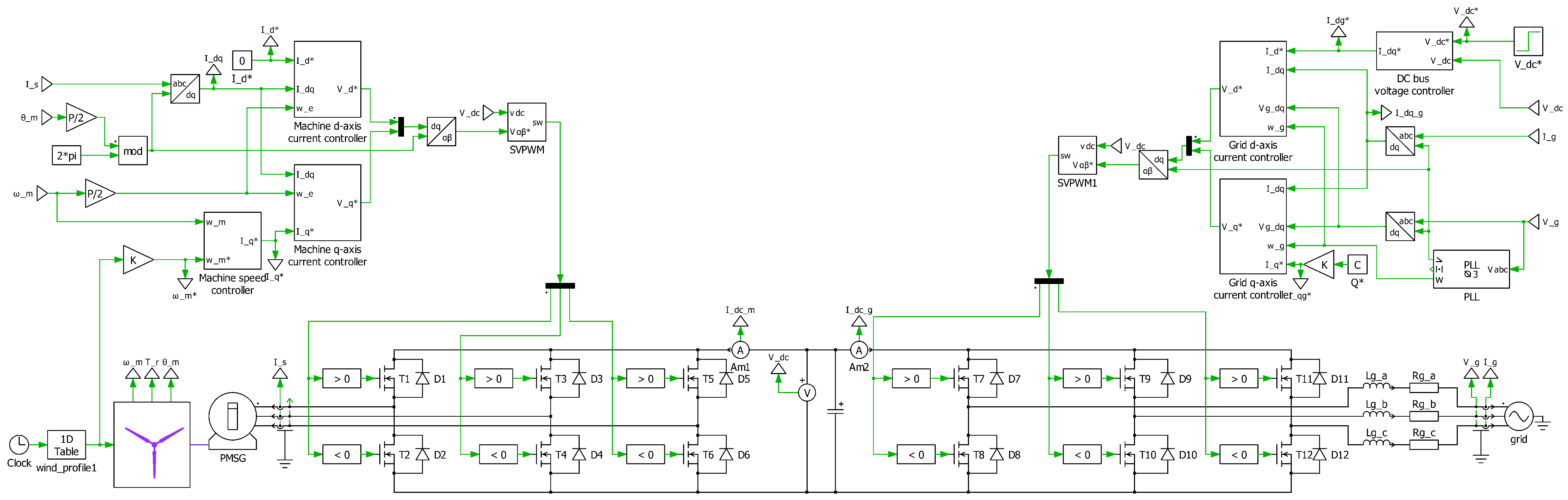
Figure 7.
Bode amplitude plot for the three controllers: (a) reference tracking of the speed controller, (b) disturbance rejection of the speed controller, (c) noise sensitivity of the speed controller, (d) reference tracking of the dc bus controller, (e) disturbance rejection of the dc bus controller, (f) noise sensitivity of the dc bus controller.
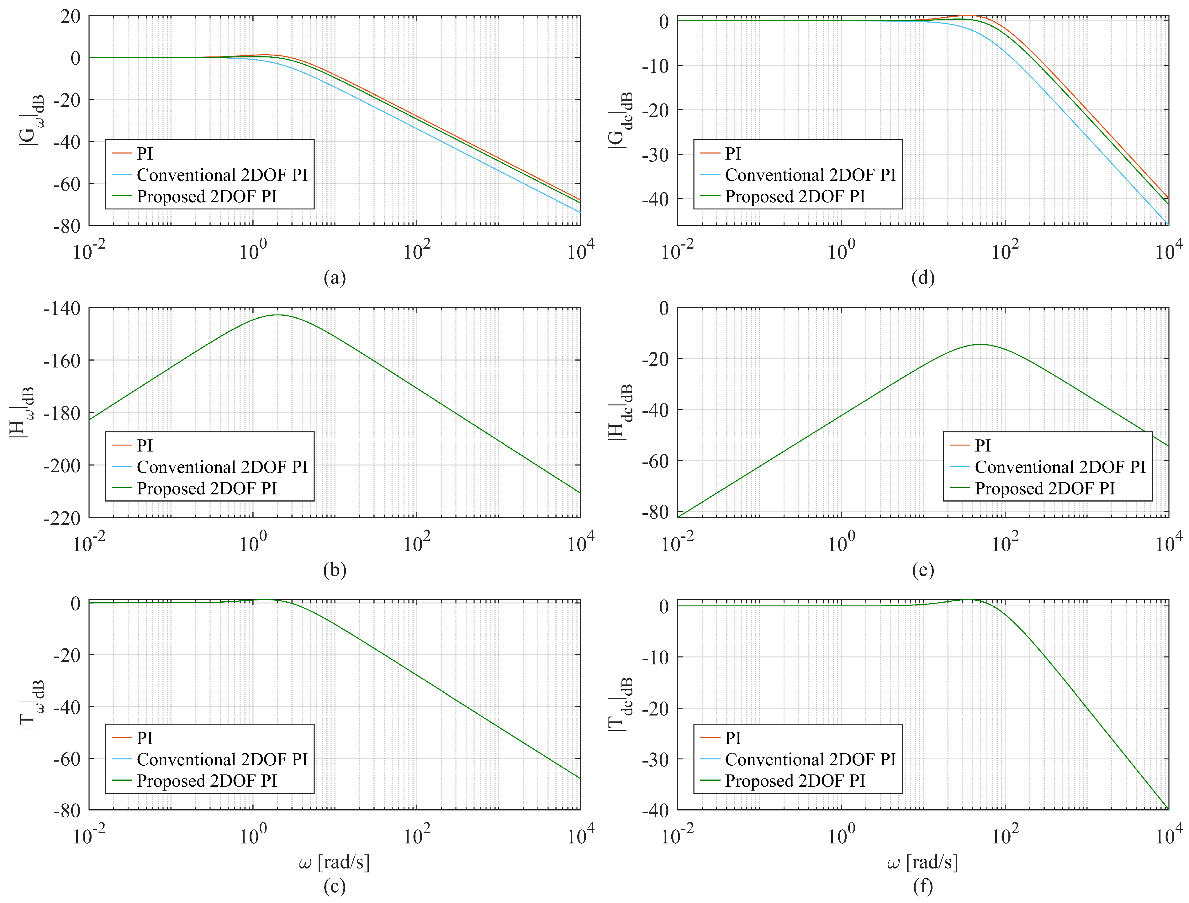
Figure 8.
Simulation results of the conventional PI controller: (a) generator speed, (b) stator d-axis current, (c) stator q-axis current, (d) DC bus voltage, (e) grid d-axis current, (f) grid q-axis current.
Figure 8.
Simulation results of the conventional PI controller: (a) generator speed, (b) stator d-axis current, (c) stator q-axis current, (d) DC bus voltage, (e) grid d-axis current, (f) grid q-axis current.
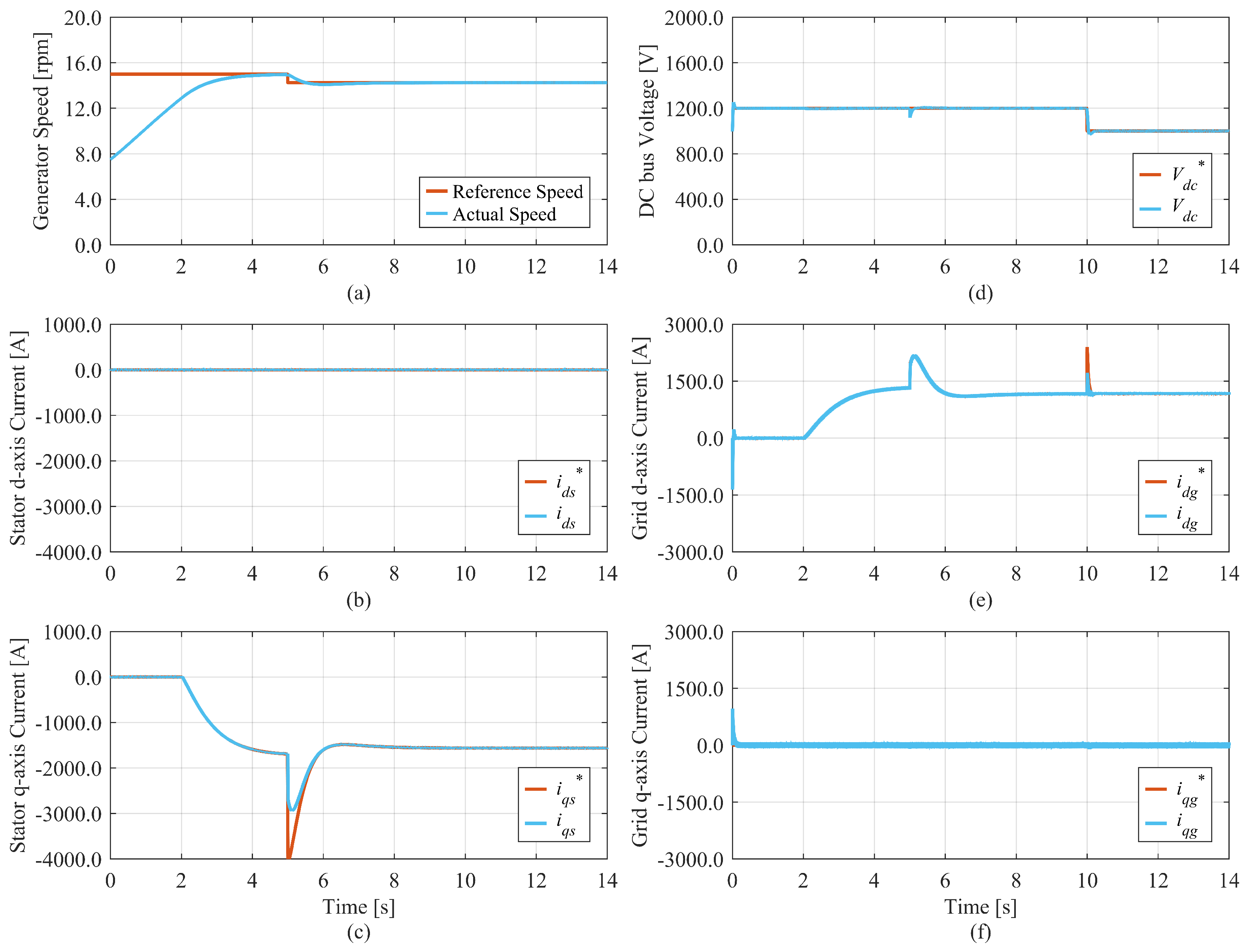
Figure 9.
Simulation results of the conventional 2DOF PI controller: (a) generator speed, (b) stator d-axis current, (c) stator q-axis current, (d) DC bus voltage, (e) grid d-axis current, (f) grid q-axis current.
Figure 9.
Simulation results of the conventional 2DOF PI controller: (a) generator speed, (b) stator d-axis current, (c) stator q-axis current, (d) DC bus voltage, (e) grid d-axis current, (f) grid q-axis current.
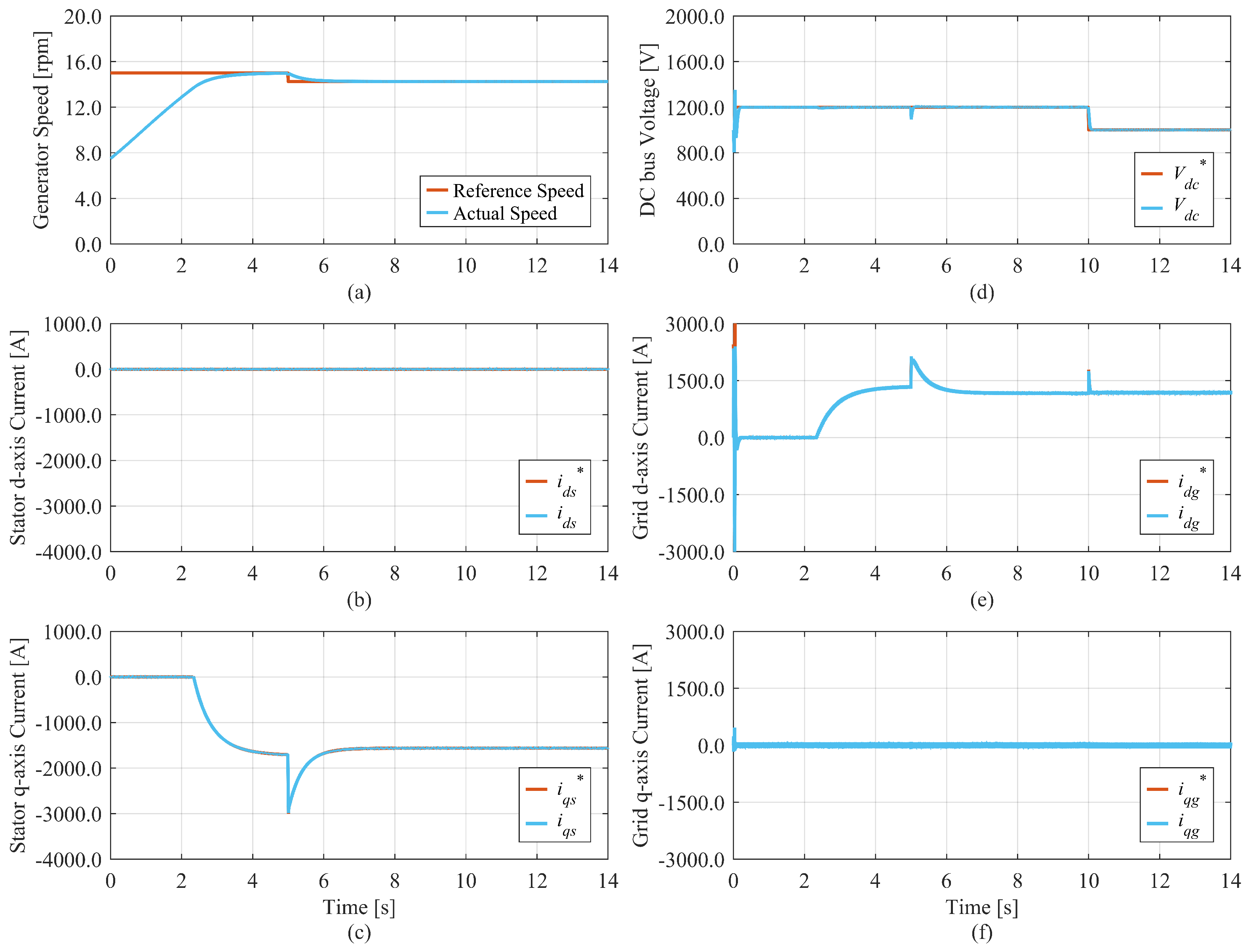
Figure 10.
Simulation results of the proposed 2DOF PI controller: (a) generator speed, (b) stator d-axis current, (c) stator q-axis current, (d) DC bus voltage, (e) grid d-axis current, (f) grid q-axis current.
Figure 10.
Simulation results of the proposed 2DOF PI controller: (a) generator speed, (b) stator d-axis current, (c) stator q-axis current, (d) DC bus voltage, (e) grid d-axis current, (f) grid q-axis current.
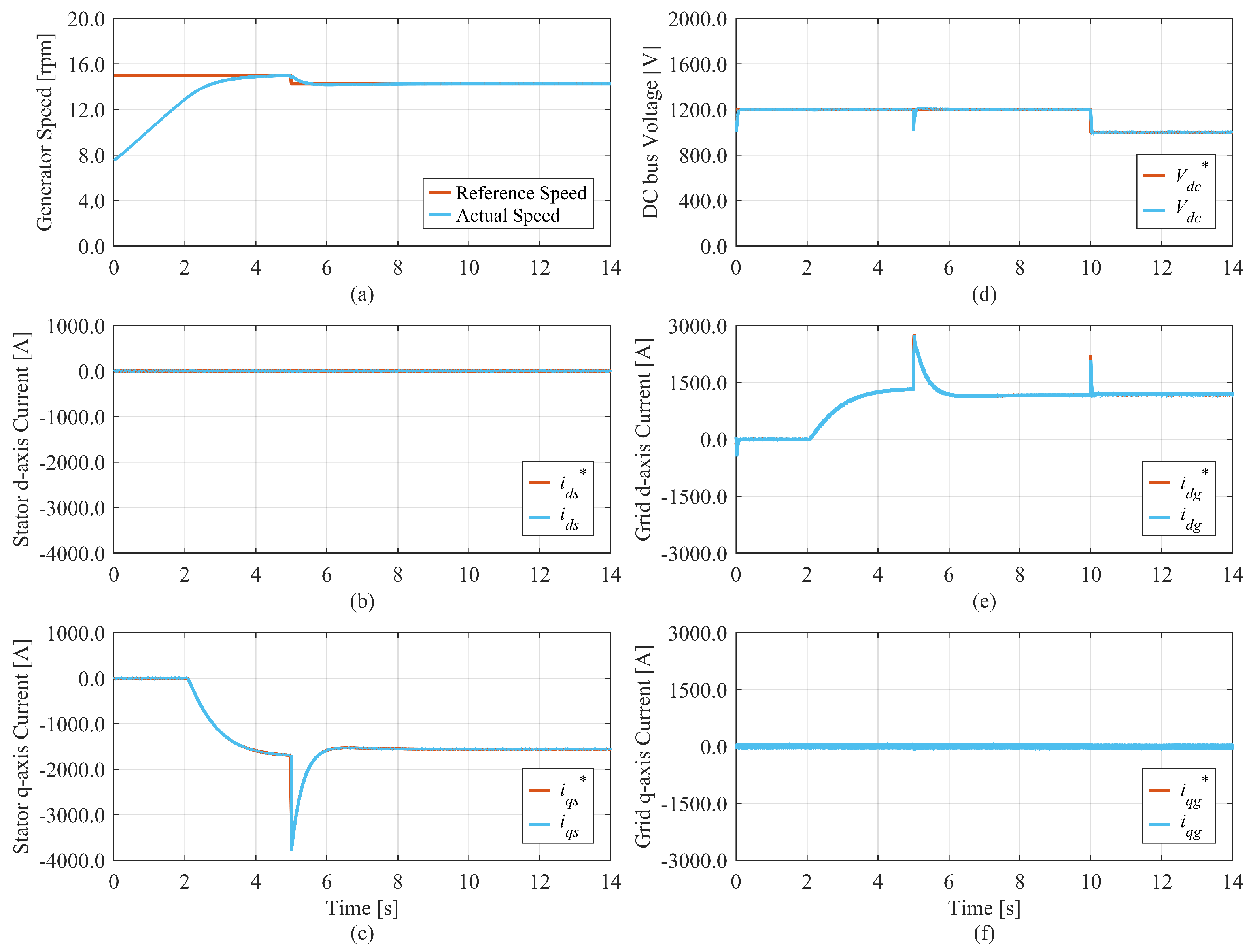
Figure 11.
Comparison of the simulation results of the conventional PI, conventional 2DOF, and the proposed 2DOF PI controller: (a) generator speed, (b) DC bus voltage.
Figure 11.
Comparison of the simulation results of the conventional PI, conventional 2DOF, and the proposed 2DOF PI controller: (a) generator speed, (b) DC bus voltage.

Table 1.
Parameters of the wind turbine subsystems.
| Model | r | y | a | b | d |
|---|---|---|---|---|---|
| stator d-axis | |||||
| stator q-axis | |||||
| mechanical | J | B | |||
| grid d-axis | |||||
| grid q-axis | |||||
| DC bus voltage | 0 |
Table 2.
Simulated system parameters.
| Parameter | Value | Units |
|---|---|---|
| Rated power | 2 | MW |
| Rated voltage | 690 | V |
| Rated speed | 18 | rpm |
| Number of poles | 60 | |
| Radius of the turbine | 41 | m |
| Optimal tip-speed ratio | 6.44 | |
| Stator resistance | 8 | mΩ |
| Stator d-axis inductance | 1.5 | mH |
| Stator q-axis inductance | 1.5 | mH |
| Moment of inertia | Kg·m2 | |
| Cut-in wind speed | 2.5 | m/s |
| Cut-out wind speed | 28 | m/s |
| Rated wind speed | 12 | m/s |
| DC-link voltage | 1200 | V |
| DC-link capacitance | 53 | mF |
| Switching frequency | 3 | kHz |
| Grid voltage | 690 | V |
Table 3.
Parameters of the speed controller and the dc-link controller.
| Generator speed controller | |||
| Parameter | PI | Conventional 2DOF PI | Proposed 2DOF PI |
| bandwidth (rad/s) | 4.9648 | 2 | 4 |
| 2 | 2 | 2 | |
| 2 | 2 | 2 | |
| z | 1 | 2 | 1.1795 |
| 2 | 2 | 2 | |
| DC bus voltage controller | |||
| Parameter | PI | Conventional 2DOF PI | Proposed 2DOF PI |
| bandwidth (rad/s) | 124.12 | 50 | 100 |
| 50 | 50 | 50 | |
| 50 | 50 | 50 | |
| z | 25 | 50 | 29.48 |
| 50 | 50 | 50 | |
Table 4.
Summary of the simulation results.
| Controller | Rise Time (s) | Maximum Percent Overshoot (%) |
|---|---|---|
| Generator speed controller | ||
| PI controller | 0.3647 | 13.5 |
| Conventional 2DOF PI controller | 1.0986 | 0 |
| Proposed 2DOF PI controller | 0.4860 | 6 |
| DC bus voltage controller | ||
| PI controller | 0.0153 | 13.5 |
| Conventional 2DOF PI controller | 0.0441 | 0 |
| Proposed 2DOF PI controller | 0.0193 | 6 |
Disclaimer/Publisher’s Note: The statements, opinions and data contained in all publications are solely those of the individual author(s) and contributor(s) and not of MDPI and/or the editor(s). MDPI and/or the editor(s) disclaim responsibility for any injury to people or property resulting from any ideas, methods, instructions or products referred to in the content. |
© 2023 by the author. Licensee MDPI, Basel, Switzerland. This article is an open access article distributed under the terms and conditions of the Creative Commons Attribution (CC BY) license (https://creativecommons.org/licenses/by/4.0/).
Share and Cite
MDPI and ACS Style
Hussain, H.A. Enhanced Control of Back-to-Back Converters in Wind Energy Conversion Systems Using Two-Degree-of-Freedom (2DOF) PI Controllers. Electronics 2023, 12, 4221. https://doi.org/10.3390/electronics12204221
AMA Style
Hussain HA. Enhanced Control of Back-to-Back Converters in Wind Energy Conversion Systems Using Two-Degree-of-Freedom (2DOF) PI Controllers. Electronics. 2023; 12(20):4221. https://doi.org/10.3390/electronics12204221
Chicago/Turabian StyleHussain, Hussain A. 2023. "Enhanced Control of Back-to-Back Converters in Wind Energy Conversion Systems Using Two-Degree-of-Freedom (2DOF) PI Controllers" Electronics 12, no. 20: 4221. https://doi.org/10.3390/electronics12204221
Note that from the first issue of 2016, this journal uses article numbers instead of page numbers. See further details here.