
Fractional Order Modeling of Thermal Circuits for an Integrated Energy System Based on Natural Transformation


1
College of Electrical Engineering, Guangxi University, Nanning 530004, China
2
Department of Mechanical and Electrical Engineering, Yangjiang Polytechnic, Yangjiang 529500, China
3
School of Computer, Electronics and Information, Guangxi University, Nanning 530004, China
*
Author to whom correspondence should be addressed.
Electronics 2022, 11(6), 914; https://doi.org/10.3390/electronics11060914
Submission received: 18 January 2022
/
Revised: 4 March 2022
/
Accepted: 14 March 2022
/
Published: 15 March 2022
(This article belongs to the Section Power Electronics)
Abstract
:With the development of the economy, energy systems have become the focus of academia and industry. The integrated energy system formed by electricity, gas, and heat networks can improve the utilization efficiency of energy. Heating networks in integrated energy systems play an important role. The consideration of the dynamic characteristics of the heating network can improve the flexibility of the system and reduce the operation cost of the system. In this paper, a thermal circuit model is derived for the heating network from an electrical-analog perspective. Based on the thermal circuit model, the fractional-order model of the thermal circuit is proposed. The Adomian polynomial decomposition method based on natural transformation is used to solve the model. The losses and transfer delays of the heating network are obtained. The computing time is about 0.5 s and the relative error is less than 0.02%. The results show that the thermal circuit analysis theory can describe the complex dynamic characteristics of heating network and that the calculation procedure is simple, fast, and accurate.
1. Introduction
Energy and environment have become important issues in current social development. Multiple energy systems represented by electricity, gas, and heat constitute an integrated energy system (IES) [1]. IES can improve the efficiency of energy utilization so as to protect the environment. Heating networks in IES play an important role in facilitating the low-cost transition to a low-carbon energy system with high penetration of renewable energy [2].
However, the dynamics of the heating network are often ignored. The transient heat transfer process that considers the heat losses and transfer delay must be taken into account. On the one hand, due to time delay, the dynamics of the heating network add complexity to the relationship between heat suppliers and demands. On the other hand, the transfer delays in heating network offer potential for heat storage. Obviously, it is necessary to properly describe the dynamics of the heating network [3]. The branch characteristics and topology constraints of the heating network were described by thermal circuit, which derived the heating network equation. The thermal circuit method can describe the thermal dynamic process in a continuous time domain [4].
IES refers to a complex system formed by the energy generation, conversion, storage, and transmission in the process of construction, planning and operation [5]. IES includes multiple energy forms, complex operation modes, and close coupling links, which bring challenges to its modeling and power flow calculation. In [6], the topological structure of the cold-heat-electric IES is given, the steady-state model of the power system, the heat system, and the energy station are established, and the unified power flow model is created. The integrated electricity and heating system has become one of the main ways to reduce carbon emissions of the power industry. With the development and application of combined heat and power (CHP) technology, the coupling effect of electrical network and heat network has been gradually strengthened [7,8]. In [9], a heat and power dispatch model is presented and an iterative algorithm is proposed to solve the problem, which improved the overall economic efficiency of the integrated heat and power system. The authors of [10] studied the physical interactions related to system safety and economic operation in an electricity-heat IES. Ref. [11] proposes a heat inertia model of the district heating systems and a flexibility assessment method of the IES. The research of heating network is of great significance to the IES, and the dynamics of heating network is very important to optimize the thermal-electric cooperation [12].
The theoretical analysis of power networks has been relatively mature, while the corresponding thermal circuit analysis theory has not yet been formed [13]. Heating network systems have some attributes such as time-delay, nonlinearity, and multi-variability, and the heat transfer process is related to many factors [14]. Some scholars have carried out research on the generalized modeling of heating networks. [15] presents a new numerical model for the simulations and analyses of the thermal transients in the district heating system. Literature [16] establishes the concept of thermal resistance based on the electric circuit analogy method and introduces an equivalent thermal circuit to represent the heat transfer process. In [17], the partial differential equation (PDE) of advection heating network is obtained by finite element method. In [18], a dynamic modeling method is proposed considering heat dissipations in pipes based on the conservation laws of mass and momentum equilibrium in one-dimensional incompressible fluid. This method can achieve high accuracy, but the calculation is large and the solution is complex.
However, in [19], researchers point out the necessity to consider the dynamics of the heating network, as the energy storage in heating network can provide flexibility for the renewables accommodation in power systems [20] considers the dynamics of heating network and only focuses on the delay between large regions in order to reduce the computational complexity. The dynamic characteristics of the urban heating network are important aspects that need to be considered for the operating scheduling [21,22] establishes the dynamic characteristic model of the urban heating network. There is no need to keep the heat source and heat load equal in the dynamic modeling of the heating network at all times. The dynamic characteristics of the heating network can give play to the heat storage characteristics [23]. The dynamic characteristics of heating network consider not only the heat losses but also the transmission delays. In [3], heat losses and transmission delays are modeled from an electrical-analog perspective, the relationship between heat source and heat load is expressed by Laplace operator, and the model is solved in the complex frequency domain. Thus, the problem that the dynamics of district heating networks have not been fully described for large transmission delay is solved. [24] expresses the relationship between the heat source and the heat load with the help of complex numbers, and solves the problem by Fourier transform, thus avoiding the calculation difficulties caused by the fact that the pipe delay and the scheduling period are not integer multiple relationship.
There are two different paradigms of the heat flow control. Control-by-temperature is adopted in China, Nordic countries, and Russia. In these systems, mass flow is adjusted rarely, and the main controls are realized by changing the temperature of the heat sources. The temperature setting changes throughout the day in order to adapt to the changes in heat demand. Control-by-mass flow is adopted in S. European countries, and the amount of heat flow is controlled by adjusting the mass flow [25].
In this paper, we use control-by-temperature. A pipeline model with distributed parameters is established from an electrical-analog perspective. A fractional-order model of the thermal circuit is proposed. The specific contributions are as follows.
- (1)
- Compared with the electricity circuit model, the thermal circuit model is studied.
- (2)
- The fractional-order model of the thermal circuit is proposed.
- (3)
- The natural transform method is used to solve the thermal circuit model.
- (4)
- The influence of different fractional orders is analyzed.
2. Thermal Circuit Analysis of Heating Network
2.1. Classical Mathematical Modeling
The typical structure of a heating network is shown in Figure 1a. The heating network includes water supply pipeline, back water pipeline, booster pump, heat station, and heat consumers. The topologies of the supply and return pipeline of the heating networks are usually symmetric. From an electric circuit-analog perspective, the relative temperature T is regarded as voltage and the heat power of the water flow h is regarded as current. The distributed parameters thermal circuit model is shown in Figure 1b [3].
Compared with the classical electric flow mathematical equation, the thermal circuit model can be expressed as:
where t is time; x is position; T is temperature; h is heat power; Rt is thermal resistance; Lt is thermal inductance; Ct is heat capacity; and Gt is thermal conductivity.
Relative temperature T is defined as the difference between absolute temperature and the surrounding environment in the water. Defining x as a space variable and t as time, the general thermal circuit model can be written as [26]:
where m is the mass flow; c is the specific heat capacity of fluid; ρ is the density; λ is the heat-loss factor of the pipeline; γ0 is radial direction thermal diffusion coefficient; S is the cross-sectional area of the heating pipeline.
Ignoring the second-order term, Equation (3) can be rewritten as Equation (4):
where m is a constant in control-by-temperature mode; h = cmT.
The parameters in Figure 1b can be obtained from Equations (1), (2) and (4):
Therefore, the thermal circuit can be compared to a circuit model from electric circuit-analog perspective. It can improve the solution efficiency of the integrated energy system. The difficulty in analysis of the heating network model will be greatly reduced if the partial differential equation is easy to solve.
2.2. Fractional-Order Mathematical Model
Scholars point out that fractional derivatives are helpful in describing linear viscoelasticity, polymeric chemistry, and so on. Moreover, fractional derivatives have proved to be a very suitable tool for the description of memory properties of various processes. Therefore, fractional-order differential equations are becoming the focus of many studies [27]. Fractional differential equations are increasingly used to model problems in research areas as diverse as mechanical systems, dynamical systems, unification of diffusion and wave propagation phenomenon and others. The advantage of using fractional differential equations is their non-local property. It is well known that the integer order differential operator is a local operator but that the fractional order differential operator is non-local. Fractional differential equations have been shown to better model complex phenomena in physics [28].
The radial direction heat-loss cannot be ignored for the large systems operating at high renumbers. At the same time, considering the influence of system geometry, water evaporation, viscosity change, and other factors, a fractional mathematical model of thermal circuit is proposed in this paper. Equation (3) is converted into fractional-order partial differential equation to time:
So, we get:
where β is fractional-order; A, B, C are determined by the following:
3. Solution Method for Solving Model Based on Natural Transformation
3.1. Natural Transformation
Various integral transformations are widely used to solve differential equations. Laplace transform is the most widely used one. Laplace transforms are widely used in many fields of engineering technology and scientific research, especially in mechanical systems, electrical systems and control systems. Sumudu transform was first proposed by Watugala in 1993 for solving differential equations. However, natural transformation has the property of converging to Sumudu and Laplace transform only by changing parameters. In many cases, complex problems are difficult to apply Laplace transform or Sumudu transform, but natural transformation methods can solve these problems [29].
The natural transform of is defined as [30]:
where u and s are the natural transform variables; t∈(−∞, ∞).
The inverse of a function’s natural transform is defined as:
where b is the real constant.
If is the nth derivative of function , then its natural transform is given by:
If is the natural transform of the function , then the natural transform of fractional derivative of order β is defined as:
3.2. Model Solving
We assume that the initial condition of Equation (7) is:
where:
Taking the natural transform of Equation (7),
So we get:
Applying the inverse natural transform,
We use the Adomian polynomial decomposition procedure:
for i = 0:
where denotes the gamma function.
Similarly:
The solution of Equation (7) can be expressed as:
3.3. Comparison with Existing Thermal Circuit Models
In this paper, the solution of the differential equation of heating network is derived by natural transformation. The solution method is similar to that in [3]. The differences between them are explained below.
In [3], a unified mathematical equation for heterogeneous energy flow in multi-energy networks is established, and a generalized circuit modeling method based on Laplace transform is proposed. The complex transmission characteristics of the multi-energy networks in time domain are transformed into a simple Laplace domain algebra problem, and the thermal circuit model of distribution parameters is proposed. The proposed model can scientifically analyze the steady-state and dynamic characteristics in the heating network. However, if the transfer delay is not integer multiple of the scheduling period, the calculation will be difficult. In [24], a thermal circuit model based on the energy conservation equation is derived for the heating network. The Fourier transform is employed to realize model simplification from partial differential equations to algebraic equations. The branch characteristics and topology constraints of the heating network is described by the thermal circuit, which derived thermal network equation further. Fourier transform is used to solve the equation in the frequency domain, which overcomes the difficulty of calculation when the transfer delay and scheduling period are not integer multiple, but it has a large amount of calculation and needs to satisfy Dirichlet condition. In this paper, the fractional differential equation of thermal circuit is proposed. The radial loss of pipeline in large-scale system is considered. An Adomian polynomial decomposition algorithm based on natural transformation is used to solve fractional differential equation.
4. Main Results and Discussion
4.1. Parameters
A pipeline is used to verify the effectiveness of the proposed model. We take the typical structure of a heating network, including a water supply pipeline and a water return pipeline, as shown in Figure 1a. Two pipes have the same parameters. The pipeline parameters are shown in Table 1. The booster pump at the heat source side operates in constant pressure mode, and its pressure increment is 0.55 MPa. The environment temperature is set to 0 °C. The opening of the flow control valve is fixed, that is control-by-temperature. We assume that the pipeline is horizontal and the pipeline length is 200 m.
4.2. Analysis and Simulation Results
It is assumed that the fractional-order at β = 1 and the temperature at the head end of the pipeline is a constant 60 °C. We compared the numerical solution of Equation (19) with the solution of the original Equation (4). The results are shown in Figure 2. It can be observed that the two curves almost coincide, and the results in this paper are very close to the results of the original equation. Table 2 shows the relative error values for i = 3 and 4. The overall relative error is less than 0.015%, which indicates that the results are accurate. The results of model operation in this paper are algebraic operation, and there is no complex iterative solution. The computing time in this paper is about 0.5 s. However, the computing time is 6 s using finite element method. So, the computing time using the proposed method is shorter.
Figure 3 presents the results by the proposed methods with step function at the head end of the pipeline and t = 5 min. T0 = 40[(exp(t)/(1 + exp(t)) + 1) is assumed to step function. It can be seen that the results of proposed method are very close to those from original partial differential equation. The results in this paper are slightly smaller than the solution of the original partial differential equation. It is mainly due to the fact that the first four terms of the polynomial solution are taken. The relative error is less than 0.02% for i = 3, which can meet the calculation requirements.
If the fractional-order values are different, the temperature curves will be different. Figure 4 shows the temperature curves at different fractional-order β = 0.8, 1, 1.3, 1.4, and the temperature at the head end of the pipeline is 60 °C. It can be seen that the higher fractional order causes a lower temperature. The results show that the fractional order has a certain impact on heat transfer. A thermodynamic constitutive equation can only reflect some main characteristics under certain conditions. The solutions of the equation are different if the conditions change. The prediction results are very similar to those of other models if the fractional order value is properly selected. For example, the movement of liquid is random when the water flow is in turbulence (that is, the velocity and pressure fluctuate irregularly with time and space) and there is water vapor in the pipe.
Figure 5 shows the results of different fractional orders at the heat-loss factor λ = 2.8. It can be seen that the changes in temperature increase. Therefore, the difference between the proposed model and the actual model can be corrected by fractional order. The proposed model will be more similar to actual model if we properly select the fractional-order.
Figure 6 shows the three-dimensional dynamic solution of pipeline temperature at different fractional-order β = 1 and 1.4. It can be seen that the temperature not only decreases with position but also changes with time. Therefore, the results of this model can dynamically display the changes of pipeline temperature with time and position.
4.3. Discussion Based on the Results
The method proposed in this paper provides a good mathematical tool for solving the dynamic characteristics of thermal circuits. However, the results based on proposed method in the heating network have certain application premise. On the one hand, we used control-by-temperature mode and it is assumed that the working fluid flow of the heating network is constant in this paper. On the other hand, the results in this paper may have certain errors since the latter terms of the polynomial are discarded. We can reduce the error by taking more terms of the polynomial.
5. Conclusions
The thermal circuit is an important part of integrated energy systems. Firstly, the time fractional-order partial differential equation of a heating network is proposed, and the fractional-order thermal circuit model is obtained. Secondly, in view of the difficulty of solving the partial differential equation in the thermal circuit, the analytical solution of the thermal circuit model is derived by using the Adomian polynomial decomposition algorithm based on natural transformation. The solution of the partial differential equation is expressed as the sum of polynomials, which reduces the difficulty of heating network analysis. If the fractional order values are different, the temperature change curves will be different. The proposed model will be more similar to an actual model if we properly select the fractional-order. Specifically, we have made the following conclusions:
- (1)
- Compared with the electric circuit model, the thermal circuit model has similar forms.
- (2)
- The proposed method reduces the computational complexity of the thermal circuit model. Compared with other models, the thermal circuit model in this paper can meet the accuracy requirements and the results can dynamically display the changes of pipeline temperature with time and position.
- (3)
- Fractional-order values have an effect on the results of heat transfer. The higher fractional-order causes a lower temperature. Different fractional-order values can be used to correspond to different conditions.
- (4)
- The model in this paper is the thermal circuit analysis theory, which is expected to contribute to the dynamic modeling of integrated energy system in the future. However, different fractional-order values correspond to different models under different conditions, which is the future research direction.
Author Contributions
Conceptualization, M.L. and J.Y.; methodology, M.L. and J.Y.; validation, M.L.; writing—original draft preparation, M.L.; writing—review and editing, J.Y.; supervision, J.Y.; funding acquisition, J.Y. All authors have read and agreed to the published version of the manuscript.
Funding
This research was funded by National Natural Science Foundation of China, grant number 61762030.
Data Availability Statement
The data presented in this study are available on request from the corresponding author.
Acknowledgments
This work was supported by Characteristic Innovation Project of Guangdong Colleges and Universities in China (2020KTSCX345).
Conflicts of Interest
The authors declare no conflict of interest.
Nomenclature
| Abbreviations | |
| IES | integrated energy system |
| CHP | combined heat and power |
| PDE | partial differential equation |
| Parameters and Variables | |
| A\B\C | refers to constant coefficient of partial differential equation |
| c | refers to the specific heat capacity |
| Ct | refers to heat capacity |
| h | refers to heat power (W) |
| Gt | refers to thermal conductivity |
| l | refers to the length of pipeline |
| Lt | refers to thermal inductance |
| m | refers to the mass flow (kg·s−1) |
| Rt | refers to thermal resistance |
| S | refers to the cross-sectional area of the heating pipeline (m2) |
| T | refers to the temperature field (°C) |
| t | refers to time |
| x | refers to the position along the pipe |
| u\s | refer to the natural transform variables |
| ρ | refers to the density (kg·m−3) |
| λ | refers to the heat-loss factor of the pipeline (W·mK−1) |
| γ0 | refers to radial direction thermal diffusion coefficient (m2·s−1) |
| β | refers to fractional-order |
| refers to the gamma function | |
References
- Li, G.; Zhang, R.; Jiang, T.; Chen, H.; Bai, L.; Cui, H.; Li, X. Optimal dispatch strategy for integrated energy systems with CCHP and wind power. Appl. Energy 2016, 192, 408–419. [Google Scholar] [CrossRef]
- Huang, B.; Hu, M.; Chen, L.; Jin, G.; Liao, S.; Fu, C.; Wang, D.; Cao, K. A Novel Electro-Thermal Model of Lithium-Ion Batteries Using Power as the Input. Electrionics 2021, 10, 2753. [Google Scholar] [CrossRef]
- Yang, J.; Zhang, N.; Botterud, A.; Kang, C. On An Equivalent Representation of the Dynamics in District Heating Networks for Combined Electricity-Heat Operation. IEEE Trans. Power Syst. 2020, 35, 560–570. [Google Scholar] [CrossRef]
- Yang, J.; Zhang, N.; Kang, C. Generalized electric circuit analysis theory for multi-energy networks. Part one branch model. Autom. Electr. Power Syst. 2020, 44, 21–32. [Google Scholar] [CrossRef]
- Cheng, H.; Hu, X.; Wang, L.; Liu, Y.; Yu, Q. Review on Research of Regional Integrated Energy System Planning. Autom. Electr. Power Syst. 2019, 43, 2–13. [Google Scholar]
- Qu, L.; Ouyang, B.; Yuan, Z.; Zeng, R. Steady-State Power Flow Analysis of Cold-Thermal-Electric Integrated Energy System Based on Unified Power Flow Model. Energies 2019, 12, 4455. [Google Scholar] [CrossRef] [Green Version]
- Chen, Y.B.; Yao, Y.; Zhang, Y. A robust state estimation method based on SOCP for integrated electricity-heat system. IEEE Trans. Smart Grid 2021, 2, 810–820. [Google Scholar] [CrossRef]
- Dong, H.; Fang, Z.; Ibrahim, A.-W.; Cai, J. Optimized Operation of Integrated Energy Microgrid with Energy Storage Based on Short-Term Load Forecasting. Electronics 2022, 11, 22. [Google Scholar] [CrossRef]
- Li, Z.; Wu, W.; Shahidehpour, M.; Wang, J.; Zhang, B. Combined heat and power dispatch considering pipeline energy storage of district heating network. IEEE Trans. Sustain. Energy 2016, 7, 12–22. [Google Scholar] [CrossRef]
- Zhaoguang, P.; Qinglai, G.; Hongbin, S. Interactions of district electricity and heating systems considering time-scale characteristics based on quasi-steady multi-energy flow. Appl. Energy 2016, 167, 230–243. [Google Scholar]
- Li, X.; Li, W.; Zhang, R.; Jiang, T.; Chen, H.; Li, G. Collaborative scheduling and flexibility assessment of integrated electricity and district heating systems utilizing thermal inertia of district heating network and aggregated buildings. Appl. Energy 2020, 258, 114021. [Google Scholar] [CrossRef]
- Guelpa, E.; Toro, C.; Sciacovelli, A.; Melli, R.; Sciubba, E.; Verda, V. Optimal operation of large district heating networks through fast fluid-dynamic simulation. Energy 2016, 102, 586–595. [Google Scholar] [CrossRef]
- Yang, J.; Zhang, N.; Kang, C. Generalized electric circuit analysis theory for multi-energy networks: Part two network model. Autom. Electr. Power Syst. 2020, 44, 15–29. [Google Scholar] [CrossRef]
- Sarafraz, M.M.; Safaei, M.R.; Tian, Z.; Goodarzi, M.; Bandarra Filho, E.P.; Arjomandi, M. Thermal Assessment of Nano-Particulate Graphene-Water/Ethylene Glycol (WEG 60:40) Nano-Suspension in a Compact Heat Exchanger. Energies 2019, 12, 1929. [Google Scholar] [CrossRef] [Green Version]
- Stevanovic, V.D.; Zivkovic, B.; Prica, S.; Maslovaric, B.; Karamarkovic, V.; Trkulja, V. Prediction of thermal transients in district heating systems. Energy Convers. Manag. 2009, 50, 2167–2173. [Google Scholar] [CrossRef]
- Chen, Q.; Fu, R.H.; Xu, Y.C. Electrical circuit analogy for heat transfer analysis and optimization in heat exchanger networks. Appl. Energy 2015, 139, 81–92. [Google Scholar] [CrossRef]
- Manson, J.R.; Wallis, S.G. An accurate numerical algorithm for adventive transport. Commun. Numer. Methods Eng. 1995, 11, 1039–1045. [Google Scholar] [CrossRef]
- Zhou, S.-J.; Tian, M.-C.; Zhao, Y.-E.; Guo, M. Dynamic modeling of thermal conditions for hot-water district-heating networks. J. Hydrodyn. 2014, 26, 531–537. [Google Scholar] [CrossRef]
- Lin, C.; Wu, W.; Zhang, B.; Sun, Y. Decentralized solution for combined heat and power dispatch through benders decomposition. IEEE Trans. Sustain. Energy 2017, 8, 1361–1372. [Google Scholar] [CrossRef]
- Wu, C.; Gu, W.; Jiang, P.; Li, Z.; Cai, H.; Li, B. Combined economic dispatch considering the time-delay of a district heating network and multiregional indoor temperature control. IEEE Trans. Sustain. Energy 2017, 9, 118–127. [Google Scholar] [CrossRef]
- Wei, W.; Shi, Y.; Hou, K.; Guo, L.; Wang, L.; Jia, H.; Wu, J.; Tong, C. Coordinated Flexibility Scheduling for Urban Integrated Heat and Power Systems by Considering the Temperature Dynamics of Heating Network. Energies 2020, 13, 3273. [Google Scholar] [CrossRef]
- Zheng, J.F.; Zhou, Z.G.; Zhao, J.N.; Wang, J.D. Integrated heat and power dispatch truly utilizing thermal inertia of district heating network for wind power integration. Appl. Energy 2018, 211, 865–874. [Google Scholar] [CrossRef]
- Wu, X.; Zhang, Q.; Chen, C.; Li, Z.; Zhu, X.; Chen, Y.; Qiu, W.; Yang, L.; Lin, Z. Optimal Dispatching of Integrated Electricity and Heating System with Multiple Functional Areas Considering Heat Network Flow Regulation. Energies 2021, 14, 5525. [Google Scholar] [CrossRef]
- Chen, B.; Sun, H.; Wu, W.; Guo, Q.; Qiao, Z. Energy circuit theory of integrated energy system analysis (II): Hydraulic circuit and thermal circuit. Proc. CSEE 2020, 40, 2133–2142. [Google Scholar]
- Chertkov, M.; Novitsky, N.N. Thermal transients in district heating systems. Energy 2019, 184, 22–33. [Google Scholar] [CrossRef] [Green Version]
- Palsson, H.; Larsen, H.V.; Ravn, H.F.; Bohm, B.; Zhou, J. Equivalent Models of District Heating Systems; Technical University of Denmark: Copenhagen, Denmark, 1999. [Google Scholar]
- Azab, M.; Serrano-Fontova, A. Optimal Tuning of Fractional Order Controllers for Dual Active Bridge-Based DC Microgrid Including Voltage Stability Assessment. Electronics 2021, 10, 1109. [Google Scholar] [CrossRef]
- He, J.H. Approximate Analytic Solution for Seepage Flow with Fractional Derivatives in Porous Media. Computer Methods in Appl. Mech. Eng. 1998, 167, 57–68. [Google Scholar] [CrossRef]
- Belgacem, F.B.M.; Silambarasan, R.; VIT University. Theory of Natural Transform. Math. Eng. Sci. Aerosp. 2012, 3, 105–135. [Google Scholar]
- Shah, R.; Khan, H.; Mustafa, S.; Kumam, P.; Arif, M. Analytical Solutions of Fractional-Order Diffusion Equations by Natural Transform Decomposition Method. Entropy 2019, 21, 557. [Google Scholar] [CrossRef] [Green Version]
Figure 1.
Heating pipeline model: (a) Schematic diagram; (b) Distributed-parameter thermal circuit model.
Figure 1.
Heating pipeline model: (a) Schematic diagram; (b) Distributed-parameter thermal circuit model.
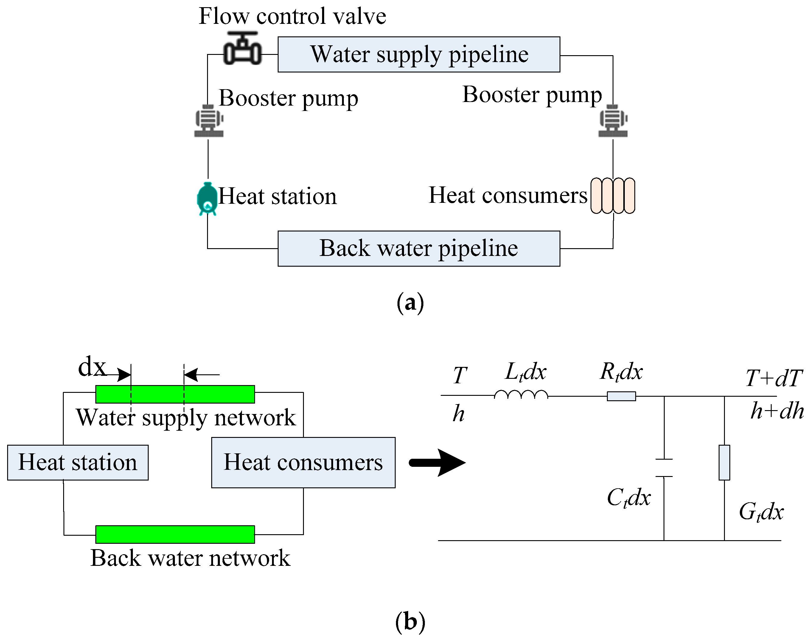
Figure 2.
Pipeline temperature with constant condition.

Figure 3.
Results with step function.
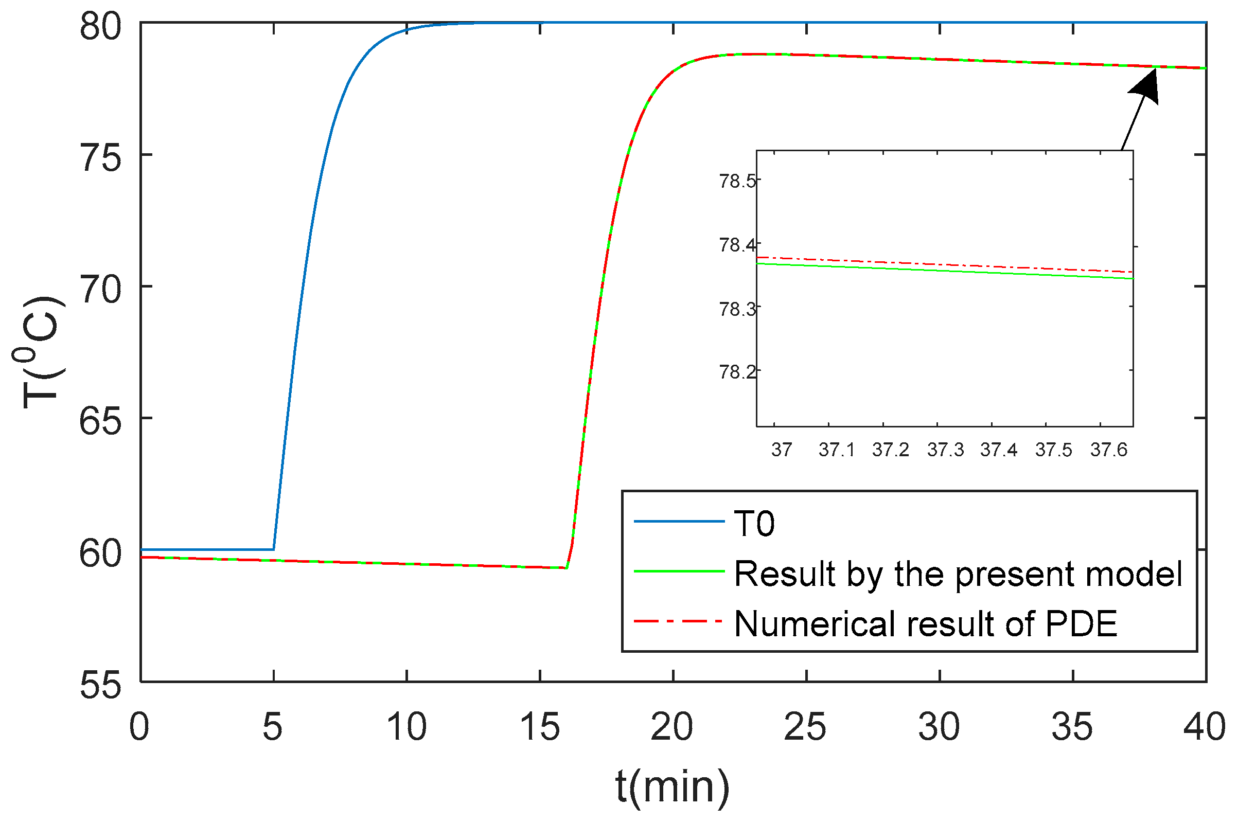
Figure 4.
Pipeline temperature at different fractional-order β = 0.8, 1, 1.3, 1.4 (λ = 0.6).
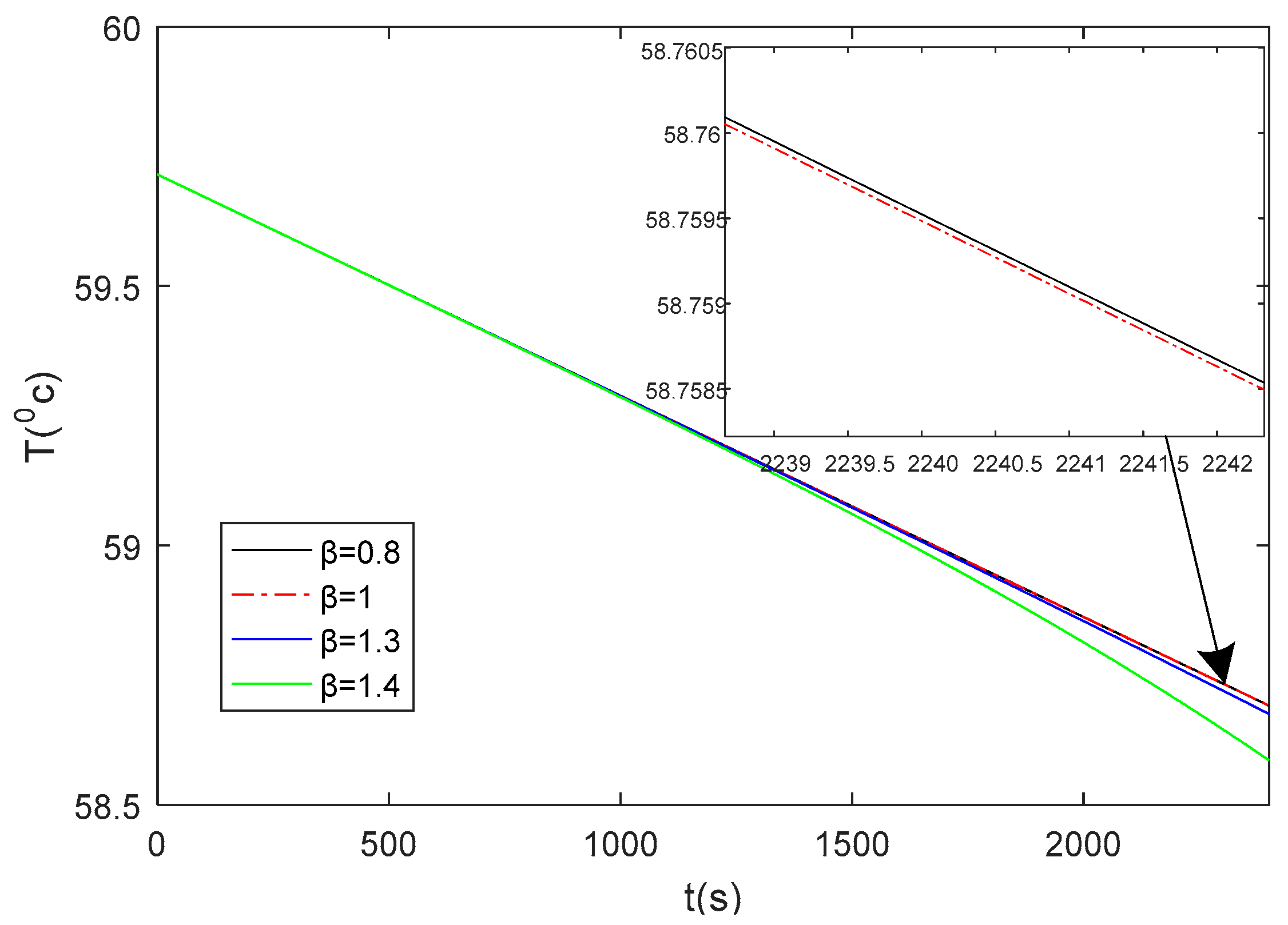
Figure 5.
Pipeline temperature at different fractional-order β = 0.8, 1, 1.3, 1.4 (λ = 2.8).

Figure 6.
Dynamic 3D map of pipeline temperature.


Table 2.
Results using natural transformation for i = 3 and 4.
| t (min) | Numerical Results of PDE | Numerical Results of Proposed Method | |||
|---|---|---|---|---|---|
| T (°C) | i = 3 | i = 4 | |||
| T (°C) | Relative Errors | T (°C) | Relative Errors | ||
| 33 | 58.87636 | 58.87039 | 0.000101 | 58.87042 | 0.000101 |
| 34 | 58.85114 | 58.8448 | 0.000108 | 58.84483 | 0.000107 |
| 35 | 58.82592 | 58.8192 | 0.000114 | 58.81924 | 0.000114 |
| 36 | 58.80071 | 58.79361 | 0.000121 | 58.79364 | 0.00012 |
| 37 | 58.77552 | 58.76801 | 0.000128 | 58.76805 | 0.000127 |
| 38 | 58.75034 | 58.74242 | 0.000135 | 58.74246 | 0.000134 |
| 39 | 58.72516 | 58.71682 | 0.000142 | 58.71687 | 0.000141 |
| 40 | 58.70000 | 58.6912 | 0.000149 | 58.69128 | 0.000149 |
Publisher’s Note: MDPI stays neutral with regard to jurisdictional claims in published maps and institutional affiliations. |
© 2022 by the authors. Licensee MDPI, Basel, Switzerland. This article is an open access article distributed under the terms and conditions of the Creative Commons Attribution (CC BY) license (https://creativecommons.org/licenses/by/4.0/).
Share and Cite
MDPI and ACS Style
Li, M.; Ye, J. Fractional Order Modeling of Thermal Circuits for an Integrated Energy System Based on Natural Transformation. Electronics 2022, 11, 914. https://doi.org/10.3390/electronics11060914
AMA Style
Li M, Ye J. Fractional Order Modeling of Thermal Circuits for an Integrated Energy System Based on Natural Transformation. Electronics. 2022; 11(6):914. https://doi.org/10.3390/electronics11060914
Chicago/Turabian StyleLi, Ming, and Jin Ye. 2022. "Fractional Order Modeling of Thermal Circuits for an Integrated Energy System Based on Natural Transformation" Electronics 11, no. 6: 914. https://doi.org/10.3390/electronics11060914
Note that from the first issue of 2016, this journal uses article numbers instead of page numbers. See further details here.