
Deep Learning Algorithms for Single Image Super-Resolution: A Systematic Review


School of Electrical & Electronic Engineering, Engineering Campus, Universiti Sains Malaysia, Nibong Tebal 14300, Pulau Pinang, Malaysia
*
Author to whom correspondence should be addressed.
Electronics 2021, 10(7), 867; https://doi.org/10.3390/electronics10070867
Submission received: 7 March 2021
/
Revised: 31 March 2021
/
Accepted: 31 March 2021
/
Published: 6 April 2021
(This article belongs to the Special Issue Deep Learning Technologies for Machine Vision and Audition)
Abstract
:Image super-resolution has become an important technology recently, especially in the medical and industrial fields. As such, much effort has been given to develop image super-resolution algorithms. A recent method used was convolutional neural network (CNN) based algorithms. super-resolution convolutional neural network (SRCNN) was the pioneer of CNN-based algorithms, and it continued being improved till today through different techniques. The techniques included the type of loss functions used, upsampling module deployed, and the adopted network design strategies. In this paper, a total of 18 articles were selected through the PRISMA standard. A total of 19 algorithms were found in the selected articles and were reviewed. A few aspects are reviewed and compared, including datasets used, loss functions used, evaluation metrics applied, upsampling module deployed, and adopted design techniques. For each upsampling module and design techniques, their respective advantages and disadvantages were also summarized.
1. Introduction
Image super-resolution is a process to recover an image of high-resolution (HR) from a low-resolution (LR) image [1,2,3,4]. In simple terms, it can also be referred to as image interpolation, scaling, upsampling, zooming, or enlarging [2]. The purpose of image super-resolution is to obtain a high pixel density and refined details from low-resolution (LR) image(s) that cannot be seen with the naked eye. Image super-resolution was very useful in applications that required recognition or detection purposes.
In the past, many image processing-based techniques have been used in image super-resolution before deep learning-based methods were started. Li et al. [5] and Nasrollahi et al. [6] classified image super-resolution methods into three different groups, namely, interpolation-based method, reconstruction-based method, and learning-based method. Several interpolation-based methods such as linear [7], bilinear [8], or bicubic [9,10] interpolations can be found in image super-resolution applications. These methods are simple, but the high-frequency details of the image are not restored and therefore more sophisticated insight may be required to recover the image [5,6].
The reconstruction-based method includes the sharpening of edge details [11], regularization [12,13], and deconvolution [14] techniques. Researchers also used these techniques for image reconstruction. The learning-based method has an advantage over the interpolation-based method by restoring the missing high-frequency details through a relationship established between the LR image and the HR image. The learning-based method can also be divided into three categories.
The first category of the learning-based method is known as neighbor embedding (NE) methods. NE assumed the local geometries property is shared between the LR image and its corresponding HR image. Therefore, the image in the HR feature domain can be computed in a form of a weighted average of local neighbors through the NE method [5]. Chang et al. [15] proposed locally linear embedding (LLE) from manifold learning, assuming two manifolds of the LR image and its corresponding HR image are locally in similar geometrics. Gao et al. [16] introduced sparse neighbor embedding (SNE) that employed a sparse neighbor scheme for super-resolution reconstruction. The idea of NE has greatly influenced the subsequent sparse coding method.
The sparse coding method is one of the learning-based methods. Sparse coding assumes the image as a sparse linear combination of elements, which can be selected from a pre-constructed and sparse enough dictionary [5]. Zhu et al. [17] demonstrated an example of using sparse coding via direction and edge dictionary for image resolution. Yang et al. [18,19] developed a sparse coding network to train a joint dictionary to find a highly sparse and over-complete coefficient matrix. The drawback of this method is that it requires memory usage and low computing speed.
With the development of machine learning technologies, research is now being extended to a new learning-based approach, which is the deep learning method. Deep learning is often applied to image processing applications, such as bank cheque verification [20], medical image processing [21], noise removal [22], and image de-hazing [23]. In 2014, the first convolution neural network (CNN) based image super-resolution algorithm was developed. Super-resolution convolution neural network (SRCNN) developed by Dong et al. [24] was the pioneer development in CNN-based algorithms. Since then, many researchers have put much effort into developing a CNN-based algorithm inspired by the idea of SRCNN.
The efforts put into the algorithm development include overcoming the model performance issues, such as gradient-vanishing problem, reducing the number of memory resources consumed, and reducing the running time of the model. From these efforts, various network design techniques were developed. These techniques include residual learning, recursive learning, multi-path learning, dense connection, and attention network.
In this paper, a systematic review is done to understand the different strategies used in previous studies. The strategies considered in this review are the datasets used for training a model, the loss function used, the evaluation metric deployed, and the network design approaches. These strategies were taken into account for this review because they are the key factors that affect the model performance, which will affect the image quality produced.
There are several surveys or reviews that have been published on deep learning-based image super-resolution algorithms. For example, Li et al. [5], Wang et al. [4], and Yang et al. [25] did comprehensive literature surveys by comparing the CNN-based method and evaluated the performance of each algorithm. In the survey done by Wang [3], and Anwar et al. [2], a list of algorithms corresponding to a network design strategy was explained. However, these reviews only explained the design and compared the performance of each network. Understanding the network design of each algorithm may not help to produce a better quality model. It is essential to understand the pros and cons or the characteristics of each network design approach to provide the correct direction to the developer to choose a correct method for development. Thus, our review paper will mainly provide:
- (1)
- A brief introduction to each proposed network
- (2)
- Pros and cons of each proposed network
- (3)
- Advantages and disadvantages for each upsampling module used
- (4)
- Pros and cons of each network design strategy deployed
2. Methodology
The systematic review was conducted using the Preferred Reporting Items for Systematic Reviews and Meta-analyses (PRISMA) standard [26]. PRISMA provided a proper guideline to select literature corresponding to related work. In this paper, IEEE Xplore and Google Scholar will be used for a comprehensive search strategy with the aid of the flowchart shown in Figure 1.
2.1. Search Strategy
The resources used for finding papers related to image super-resolution were IEEE Xplore and Google Scholar. The search was performed from 2014 to January 2021 with specific keywords as the searching index. IEEE Xplore (https://ieeexplore.ieee.org/Xplore/home.jsp) (access on 1 January 2021) is a digital library database that stores several journals, conference papers, and magazines. The keywords used for the IEEE Xplore searching index were “image super resolution” AND (“deep learning” OR “CNN”) with the combination of operator AND. A total of 850 records were found in the IEEE Xplore database using the condition specified.
As for Google Scholar (https://scholar.google.com/) (access on 1 January 2021), it is a public platform owned by Google that allows users to search different articles that correspond to the keywords inserted. The keyword “image super resolution deep learning” was used as a key index, and a total of 1000 records were found.
2.2. Study Selection
A total of 1850 articles were found, in which 850 records from IEEE Xplore and 1000 records from Google Scholar. Among these articles, 1150 articles were found to be duplicated and were filtered out. The remaining 700 articles were screened on their title and abstract. The articles were included in the systematic review if the following conditions were met: (a) an original article that developed an algorithm; (b) the development was not restricted to a particular application, such as medical diagnosis, surveillance, biometric information identification, and so on; (c) it had to follow standard datasets, such as T91, Set5, Set14, DIV2K, BSDS100, BSDS200, Manga109, and Urban100; (d) article that involved developing a new algorithm; and (e) it had to be a deep learning-based algorithm.
After the screening process, 660 records were filtered out as they did not meet the requirements, leaving 40 articles. The articles were further excluded when the following criteria were not met: (a) unclear model set-up details, such as the number of epochs, optimizer, and loss function used; (b) no model architecture is shown; (c) non-CNN-based network. Among the 40 articles, 20 articles were due to unclear model details, one article was due to model architecture not shown, and another article was due to recurrent neural network (RNN)-based network was used. Therefore, a total of 18 articles were left to be included in the systematic review.
From these 18 articles, the network design used by each article will be compared and reviewed, including the pros and cons of each design deployed. Besides that, the summary details of datasets, loss function, and evaluation metrics used in the researches will be reviewed as well.
3. Results
This section will discuss the relevant works on image super-resolution techniques that have been proposed by researchers. Section 3.1 will discuss the type of datasets being used by researchers for image super-resolution development. In Section 3.2, the loss function that is introduced into the model training as learning strategies will be summarized. Next, the performance metric to evaluate the model performance will be studied in Section 3.3. Lastly, the algorithm techniques developed by different researchers will be compared and reviewed in Section 3.4.
3.1. Datasets
A dataset is commonly used in machine learning applications, including deep learning, to teach a model network to solve a specific problem. In the image super-resolution development field, there are various types of datasets being used by many researchers to build a model and to test the model performance. From the 18 articles that have been reviewed, 11 datasets were discovered.
The T91 dataset that contains 91 images is one of the image datasets used for model training. The T91 dataset has an average resolution of 264 × 204 pixels and average pixels of 58,853. The contents in the dataset are made up of car, flower, fruit, human face, and so on [3]. SRCNN [24], fast super resolution convolution neural network (FSRCNN) [27], very deep super resolution (VDSR) [28], deep recursive convolution network (DRCN) [29], deep recursive residual network (DRRN) [30], global learning residual learning (GLRL) network [31], deep residual dense network (DRDN) [32] and fast global learning residual learning (FGLRL) network [33] are the algorithms that used T91 datasets as a training dataset.
Since the number of images in T91 was insufficient for the training purpose, some researchers included the Berkeley segmentation dataset 200 (BSDS200). The BSDS200 dataset contains images of animals, buildings, food, landscape, people, and plants as content. A total of 200 images can be found in this dataset with an average resolution of 435 × 367 pixels, and average pixels of 154,401 [34]. VDSR, DRRN, GLRL, DRDN, and FGLRL were the models built with BSDS200 as an additional training dataset. However, for FSRCNN, this dataset was used as a testing dataset. Dilated residual dense network (Dilated-RDN) [35] was another algorithm that used BSDS200 for training the model.
Another dataset that is widely used by many researchers is the DIVerse 2K resolution (DIV2K) image dataset. DIV2K dataset consists of 800 training images and 200 validation images. The images have an average resolution of 1972 × 1437 pixels and average pixels of 2,793,250. Environment, flora, fauna, handmade objects, people, and scenery are the key items found in the dataset [36]. Enhanced deep residual network (EDSR) [37], multi-connected convolutional network for super-resolution (MCSR) [38], cascading residual network (CRN) [39], enhanced residual network (ERN) [39], residual dense network (RDN) [40], Dilated-RDN [35], dense space attention network (DSAN) [41] and dual-branch convolutional neural network (DBCN) [42] were the algorithms that used the DIV2K dataset as their training dataset.
The ImageNet dataset is also used in two algorithms among the 18 articles. Efficient sub-pixel convolutional neural network (ESPCN) [43] and super resolution dense connected convolutional network (SRDenseNet) [44] were the two algorithms that use this dataset to train a model. The ImageNet dataset is one of the largest datasets with more than 3.2 million images that are open publicly for data analytics development purposes [45]. The ImageNet dataset contains images of mammals, birds, fish, reptiles, amphibians, vehicles, furniture, musical instruments, geological formations, tools, flowers and fruit.
The DIV2K and BSDS200 datasets were also used as testing datasets to evaluate model performance. EDSR, MCSR, CRN, ERN, and RDN included DIV2K for model evaluation, whereas FSRCNN, ESPCN, and DRDN included BSDS200 to evaluate the model. There are two datasets, which are Set5 and Set14, used by all algorithms, except for MCSR and DRDN, for model evaluation. The Set5 dataset contained only five images, which are images of a baby, a bird, a butterfly, a head, and a woman. The images are in PNG format at an average resolution of 313 × 336 pixels and average pixels of 113,491. The Set14 dataset consisted of 14 images with key items of humans, animals, insects, flowers, vegetables, comics, and slides. The average resolution and average pixels of the images in this dataset were 492 × 446 pixels and 230,203, respectively.
Three more types of datasets were also found to be used for model evaluation. They were the Berkeley segmentation dataset 100 (BSDS100), Urban100, and Manga109 [46]. BSDS100 was used by VDSR, EDSR, CRN, ERN, DRCN, DRRN, GLRL, FGLRL, SRDenseNet, RDN, Dilated-RDN, DBCN, and SICNN as testing dataset. This dataset contained 100 images with key contents of animals, buildings, food, landscapes, people, and plants. Meanwhile, Urban100 contained 100 images and an average resolution of 984 × 797 pixels with average pixels of 774,314. The contents of the images were related to objects, such as architecture, cities, structures, and urban. It was used by VDSR, EDSR, CRN, ERN, DRCN, FGLRL, SRDenseNet, RDN, Dilated-RDN, DBCN, and SICNN.
The Manga109 dataset was a dataset with manga volumes [47]. There were 109 PNG format images found in this dataset at an average resolution of 826 × 1169 pixels and average pixels of 966,111. Only RDN and SICNN included Manga109 datasets as testing datasets for the model. Table 1 summarizes the characteristics of datasets that have been used in image super-resolution algorithm development. Table 2 lists all the algorithms with their corresponding training and testing datasets. In Table 2, the label “T” stands for training dataset, whereas “E” stands for evaluation or testing dataset.
3.2. Loss Function
A loss function is a type of learning strategy used in machine learning to measure prediction error or reconstruction error, and it provides a guide for model optimization [3]. Two common loss functions were found in the 18 articles. One of the loss functions was a mean square error (MSE), which is also known as L2 loss. MSE can be expressed as in Equation (1).
where h is the height of the image, w is the width of the image, c is the number of channels of the image, was the constructed individual pixels value at row i, column j and channel k, was the original individual pixel value. L2 loss is good for a model to get a high peak-signal-to-noise ratio (PSNR) [48], an indicator to evaluate model performance which will be discussed in Section 3.3. SRCNN, FSRCNN, ESPCN, VDSR, DRRN, GLRL, DRDN, FGLRL and SRDenseNet were the algorithms that use MSE as learning strategies.
Another type of loss is the mean absolute error (MAE), also known as L1 loss. Although L1 loss may not help the model in achieving a better PSNR as compared to L2 loss, L1 loss provides a powerful accuracy and convergence ability to the model [39]. EDSR, CRN, ERN, DRCN, RDN, Dilated-RDN, DSAN, DBCN, and SICNN were using MAE as learning strategies during the model training. MAE can be expressed as in Equation (2).
MCSR proposed a custom loss function capable of coping with the outliers properly, which MSE and MAE cannot do. The proposed loss function, L(r,α,β) was defined as in Equation (3)
where r is the pixel-wise error between predicted and actual HR images, ρ(α) = max(1,2-α), α is the shape parameter that controls the robustness of the loss, and β is the scale parameter that controls the size of the loss’s quadratic bowl. Equation (3) was a generalized equation that can be represented as L1 loss, L2 loss, Charbonnier loss (L1 − L2 loss) by changing the value of α [49]. For example, when α = 2, Equation (3) will behave similarly to the L2 loss. When α = 1, Equation (3) will behave like the L1 loss. Therefore, the tunable parameters provided a flexibility to the model to minimize the loss value and optimizing the training process without constraining use to a single type of loss function. As such, MCSR used α = 1.11 and β = 0.05 as the loss function settings. Table 3 summarized all the algorithms corresponding to the loss function used.
3.3. Evaluation Metrics
Evaluation metrics provided an indicator to researchers to evaluate the model performance developed. It is also a standard benchmarking so that the performance between the different models can be compared. Two types of metric indicators were found, which were the peak signal-to-noise ratio (PSNR) and structural similarity (SSIM).
PSNR was used to measure the quality of the reconstruction image [3]. It was defined as the ratio of the maximum pixel value over the mean squared error between the original image and the reconstructed image. In simple expression, PSNR can be expressed as in Equation (4):
where L was the maximum pixel value (equals to 255 when an 8-bit pixel value was used), N was the number of images, was the original image, and was the reconstructed image.
SSIM measured the structural similarity between images in terms of luminance, contrast, and structures [3]. The comparison expression for luminance and contrast denoted as and can be obtained from Equations (5) and (6), respectively:
where is the mean value of the original image intensity, is the mean value of the reconstructed image intensity, is the standard deviation of the original image intensity, and is the standard deviation of the reconstructed image intensity. and were the constants for avoiding instability, which were expressed as and , respectively, where k1 << 1 and k2 << 1.
Image structure was related to the correlation coefficient between the original image I and the reconstructed image . Therefore, for structure comparison, it can be obtained from Equation (7):
where was the covariance between and that can be expressed as Equation (8) and C3 was the constant for stability.
From Equations (5)–(7), SSIM can be calculated as in Equation (9):
where α, β, and γ were the control parameters for adjusting the importance of luminance, contrast, and structure, respectively. Table 3 visualized the evaluation metrics used by different algorithms.
3.4. Algorithms
In this subsection, a total of 18 algorithms will be reviewed. Their network design deployed and the results obtained will be compared.
3.4.1. Super-Resolution Convolutional Neural Network (SRCNN)
SRCNN was the pioneering work of using a convolutional neural network (CNN) in image super-resolution reconstruction development [24,48]. The idea of SRCNN was inspired by sparse coding-based super-resolution methods. SRCNN consisted of three main parts, namely patch extraction, non-linear mapping, and image reconstruction, which can be observed in Figure 2. The patch extraction extracts features from the bicubic interpolation. Extracted features were then passed through non-linear mapping, where each of the high-dimensional features was mapped on another high-dimensional feature. Finally, the output feature from the last layer of non-linear mapping was reconstructed into the HR image through the convolution process.
When comparing SRCNN with sparse coding-based methods, they have similar operations, which include patch extraction, non-linear mapping, and image reconstruction. The difference observed between them was that the filters in SRCNN were available for optimization through end-to-end mapping, but in a sparse coding-based method, only certain operations were. Another advantage observed from SRCNN was that different filter sizes can be set in non-linear mapping, and therefore the whole operation can utilize the information obtained. These two advantages have shown that the PSNR value of SRCNN was greater than the sparse coding-based method.
3.4.2. Fast Super-Resolution Convolutional Neural Network (FSRCNN)
Dong et al. [27] later discovered that SRCNN required more convolutional layers in the non-linear mapping to get a better result. However, increasing the number of layers increases the running time, and is difficult for the PSNR value to converge during the training process. Therefore, FSRCNN was proposed to overcome these problems. FSRCNN contained five major parts, shown in Figure 3, namely, feature extraction, shrinking, non-linear mapping, expanding, and image reconstruction. One of the differences in FSRCNN from SRCNN was the addition of a shrinking layer and an expanding layer in FSRCNN. The shrinking layer reduces the dimension of extracted features from the previous layer. Meanwhile, the expanding layer works in reverse to the shrinking process, where it expands the output feature of the last layer in non-linear mapping. Besides, FSRCNN used deconvolution as an upsampling module.
FSRCNN was significantly proven that its PSNR value achieved a 1.3% improvement compared to SRCNN. Besides, FSRCNN also achieved an average 78% reduction in running time compared to SRCNN. The improvements were due to the following changes: (a) deconvolutional kernel was used instead of bicubic interpolation which proved that deconvolutional kernel outperformed the bicubic kernel; (b) shrinking layer was used, which reduced the overall number of parameters in the model, which saved training time and reduced memory consumption; (c) number of filters used in FSRCNN was less than that in SRCNN, which in turn improved the model performance and reduced running time; (d) filter size in FSRCNN was smaller than SRCNN, resulting in fewer parameters and the network was able to train more efficiently in a shorter time.
3.4.3. Efficient Sub-Pixel Convolutional Neural Network (ESPCN)
ESPCN was developed to overcome the complexity issue in SRCNN as it grew quadratically. This drawback in SRCNN caused high computation cost with a factor of n2 when upscaling factor, n, was applied to LR image using bicubic interpolation. Besides, the interpolation method did not bring additional information to solve the ill-posed reconstruction problem [43]. The design of ESPCN is shown in Figure 4. The design was the same as that in SRCNN, exception for the upsampling module. In ESPCN, sub-pixel convolution was used instead of bicubic interpolation.
The deployment of sub-pixel convolution in ESPCN has demonstrated a positive result in PSNR value compared to SRCNN. It was observed that the weight of the first layer filter and the last layer filter in ESPCN after using sub-pixel convolution has a strong similarity in terms of their features. Shi et al. [39] performed an additional experiment to compare the effect of using a tanh function and rectifier linear unit (ReLU) as activation functions after the sub-pixel convolution. As a result, the tanh activation function showed better results when compared to the ReLU activation function.
3.4.4. Very Deep Super Resolution (VDSR)
The network design of VDSR is shown in Figure 5. It was proposed by Kim et al. [28] to overcome the problem of requiring more mapping layers to get better model performance in SRCNN. VDSR introduced residual learning between the input and output of the final feature mapping layer. Residual learning added output features from the final layer to the interpolated features through a skip connection. Since low-level features and high-level features are highly correlated, the skip connection helped to utilize the features from the low-level layer by combining them with the high-level features and improved the model performance. Therefore, the skip connection was able to solve the vanishing gradients problem caused by the increasing number of layers in the model. The deployment of residual learning in VDSR has two benefits over SRCNN. First, it helped the network to achieve convergence in a shorter time since the LR image has a high correlation with the HR image. A total of 93.9% reduction in running time was observed in the VDSR model. Second, VDSR provided a better PSNR value than SRCNN.
3.4.5. Enhanced Deep Residual Network (EDSR)
Inspired by the residual network in VDSR and network architecture in SRResNet, EDSR was proposed to overcome the problem of heavy computation time and memory consumption due to the application of bicubic interpolation as an upsampling technique [37]. EDSR as showed in Figure 6 contained three major modules, which were feature extraction, residual block module, and upsampling module. The idea of the residual block came from SRResNet, whereas the skip connection idea was from VDSR. Within the individual residual block, residual learning was also applied between the input and output features. The difference between VDSR and EDSR was that some of the layers in VDSR were replaced with residual blocks. Besides, EDSR used sub-pixel convolution as an upsampling module while VDSR used bicubic interpolation. As compared to SRResNet, batch normalization (BN) layers were removed in the residual block in the EDSR model.
EDSR utilized the information from each residual block by introduced residual learning within the block, and this significantly improved the PSNR value by about 3.84% compared to VDSR. Besides, the adoption of sub-pixel interpolation also helped model performance improvement, other than computation time and memory consumption reduction. By comparing with SRResNet, removing BN that contained the same amount of memory as the preceding convolution layer also saved about 40% of memory usage during the training process. Besides, removing BN can improve model performance as BN will get rid of the range of flexibility after normalizing the features.
3.4.6. Multi-Connected Convolutional Network for Super-Resolution (MCSR)
Chu et al. [38] mentioned that EDSR failed to utilize the low-level features although it reduced the vanishing-gradient problem, in which EDSR still has the potential to get better performance. Besides, the residual learning in VDSR is only adopted in between the first layer and last layer of non-linear mapping in which the performance may degrade. Therefore, MCSR, with network design shown in Figure 7, was developed to overcome the problems. Instead of using a single path network in the residual block from EDSR, MCSR modified it to a multi-connected block (MCB) that used a multi-path network. In MCSR, the residual learning used the concatenation technique to concatenate features instead of adding the features as in EDSR.
The custom design loss function used in MCSR provided flexibility to the model to minimize loss value and optimized the training process. As a result, MCSR showed an improvement of 0.79% in PSNR value compared to EDSR. Besides the help from the loss function, the improvement made was also due to rich information in local features (feature in multi-connected block) being extracted and combined with high-level features via concatenation.
3.4.7. Cascading Residual Network (CRN)
Recently, Lee et al. [39] designed CRN, as shown in Figure 8, to overcome the massive parameters in the EDSR network structure caused by increasing depth substantially to improve the performance of the EDSR model. The network design of CRN was also inspired by the EDSR network by replacing the residual block in EDSR with a locally sharing group (LSG). The LSG consisted of a number of local wider residual blocks (LWRB). LWRB were the same as the residual block in EDSR except that the number of the channel used in the convolutional layer before ReLU activation was bigger, whereas a smaller channel was used in the second convolutional layer. Each LSG and each LWRB were adopted with the residual learning network, which can be observed in Figure 8.
The experiment showed that the performance of the CRN model was comparative with the EDSR model. Although the PSNR value of CRN was slightly lower than that in EDSR, CRN performed four times faster than EDSR. This is because CRN utilized all the features, including LWRB, with the aid of residual learning. As a result, CRN required smaller depth to achieve the close performance to EDSR, and thus shorter time was required to achieve convergence in PSNR value. For example, EDSR used 32 residual blocks; while CRN used 4 LSGs with each LSG made up of 4 LWRBs, which is equivalent to 16 residual blocks.
3.4.8. Enhanced Residual Network (ERN)
Lee et al. [39] also proposed another network called ERN, which performed slightly better than CRN. The structure of ERN was also an idea coming from EDSR with an additional skip connection between LR and output of the last LWRB via multiscale block (MSB), which has been illustrated in Figure 9. The purpose of MSB was to extract low-level features directly from the original image at different scales. Instead of using LSG, ERN deployed LWRB in non-linear mapping.
By comparing ERN with EDSR, ERN’s performance still has some small gaps to achieve the same performance as EDSR. However, ERN worked better than CRN. Since ERN only used 16 LWRBs in the model, which was a significantly smaller depth compared to EDSR, CRN has a shorter running time, which is four times faster than EDSR. As both CRN and ERN adopted residual learning to utilize all the feature information from low levels in the network, this also became one of the benefits over FSRCNN and ESPCN.
3.4.9. Deep-Recursive Convolutional Network (DRCN)
DRCN was the first algorithm that applied a recursive method for image super-resolution [29]. As shown in Figure 10, DRCN consisted of three major parts, namely embedding net, inference net, and reconstruction net. The embedding net extracted features from the interpolated image. Extracted features were then passed through an inference net in which all the filters sharing the same weight. All the intermediate outputs from each convolutional layer in the inference net and interpolated features were convoluted before they were added together to form an HR image.
DRCN was designed to overcome the problem of requiring many mapping layers to achieve better performance in SRCNN. Since the recursive method was used, shared weight allowed the network to widen the receptive field without increasing the model capacity, and therefore, fewer resources were required during the training process. Besides, the assembling of all intermediate outputs from the inference net significantly improved the model. The residual learning was also included in the network, which gave additional benefit to the model to achieve better convergence. Overall, an improvement of 2.44% was observed in DRCN compared to SRCNN.
3.4.10. Deep-Recursive Residual Network (DRRN)
Two drawbacks were observed from DRCN; one of them was that DRCN requires supervision on every recursion, which was a burdening process. Second, there was only a single type of weight being shared among all convolutional layers in the inference net. With these drawbacks observed, DRRN was developed with the network structure shown in Figure 11a. By using the basic idea from DRCN, the inference net was replaced with the recursive block. The recursive block consisted of multiple residual units, with each residual unit having two convolutional layers. One of the convolutional layers in each residual unit (light blue block in Figure 11b) shared the same weight, while the other convolutional layers (light green block in Figure 11b) shared the other same weight.
The PSNR value of DRRN showed a 0.7% improvement compared to DRCN. The improvement made was observed for the following points. First, the involvement of residual learning in the residual block helped to solve the degradation problem affecting the model performance. Second, many computation resources can be saved as many layers share the same weights. Besides that, DRRN relieved the burden of supervision on every recursion by designing a recursive block with a multi-path structure.
3.4.11. Global Learning Residual Learning Network (GLRL)
Inspired by the work in SRCNN, DRCN, and DRRN, GLRL was developed by Han et al. [31] with the network structure illustrated in Figure 12. GLRL combined the basic design from SRCNN, intermediate output design from DRCN, and recursive block design from DRRN. In non-linear mapping, a local residual block (LRB) was used, and each residual block has a similar structure with the recursive block in DRRN. Some modifications have been made for the residual block. First, a parameter rectifier linear unit (PReLU) was applied after the convolutional layer. Second, an additional process was made to the input feature before they were added to each residual unit. All the intermediate outputs from each local residual block performed a similar step as in DRCN for reconstruction purposes.
A comparison has been made between SRCNN and GLRL in terms of their PSNR value. The results showed that GLRL achieved a 0.8% improvement as compared to SRCNN. An additional experiment was carried out to compare the effect of the number of LRB on the model performance. The greater the number of LRBs, the better the performance of the model. The adoption of the PReLU layer consisted of a learnable negative coefficient able to avoid the “death structure” caused by zero gradients in the ReLU.
3.4.12. Fast Global Learning Residual Learning Network (FGLRL)
Han et al. [33] later extended their work to modify the network structure in GLRL, and FGLRL was created. In GLRL, SRCNN design was used as a base design, but in FGLRL, FSRCNN was used as a base design. Therefore, FGLRL consisted of five parts, as shown in Figure 13, which were patch extraction, shrinking, non-linear mapping, expanding, and reconstruction. PReLU was used as an activation function in this network. In GLRL, bicubic interpolation was used as upsampling kernel, whereas, in FGLRL, the deconvolutional layer was used in the upsampling module.
FGLRL worked better in the Set5 dataset at the scale factor when compared to the DRCN model. When compared to GLRL, FGLRL showed a 1.3% improvement in PSNR value. Although the model performance of FGLRL may not be satisfactory, the model running time still got the advantage over DRCN and GLRL. FGLRL was running two times faster than DRCN and GLRL. This is because the shrinking layer that reduced the dimension of patch extraction features helped to reduce memory resources and running time.
3.4.13. Deep Residual Dense Network (DRDN)
In DRRN, the skip-connection is only applied between the input feature and the output of the residual unit. DRRN was modified for further improvement, and DRDN was created. DRDN’s structure is illustrated in Figure 14. DRDN consisted of shallow feature extraction, residual dense network, and fusion reconstruction. Since the dense connection was introduced within the residual block, the residual block in DRDN was also known as a dense block (DB). Fusion reconstruction concatenated all the intermediate output from each dense block before the HR image was reconstructed.
Dense connection brought all the input features to all inputs of each convolutional layer. Besides, every output from each convolutional layer will also be brought to the input of the subsequent layer. Therefore, a dense connection linked all the features from each of the convolutional layers within the DB. DRDN benefitted in terms of computing cost and ran faster than DRRN because the number of network layers used in DRDN was less than that in DRRN. Besides, the combination of all intermediate outputs from the dense block at different depths helped the model to converge faster, which was two times faster than DRRN.
3.4.14. Super Resolution Dense Connected Convolutional Network (SRDenseNet)
In SRCNN and VDSR, these two networks did not fully utilize all the features, especially only involving the high-level features at the very deep end for reconstruction. This may be caused by loss of rich information, and the model performance will be limited. Therefore, SRDenseNet, as shown in Figure 15, was proposed to overcome the problem. SRDenseNet design was inspired by the idea of DenseNet that has the capability of improving the flow of information through the network. Five major parts were performed in the network design, namely, feature extraction, residual dense network, bottleneck layer, upsampling module, and reconstruction module. In the residual dense network, the individual dense block contained a series of convolutional process with deployed dense connections.
SRDenseNet improved the PSNR value by about 4.3% when compared to SRCNN. The model also improved the PSNR value by 2.0% when compared to VDSR and DRCN. Therefore, the adoption of dense connection in dense blocks significantly showed that it was able to solve the gradient vanishing problem, which often happens when the network becomes deeper. Besides, the adoption of the deconvolutional layer also helped in improving the reconstruction process since the layers are able to learn the upscaling filters.
3.4.15. Residual Dense Network (RDN)
SRDenseNet still had a minor disadvantage, although it performed well compared to SRCNN, VDSR, and DRCN. The disadvantage was that the mode will be hard to train when it got wider with dense blocks. Thus, RDN [40] was proposed, with its network design shown in Figure 16. In RDN, residual dense block (RDB) was used instead of DB. Other than dense connection, residual learning is also adopted within RDB. The residual learning in RDB is also known as local residual learning. Other than that, the intermediate output from each RDB was fused through concatenation before global residual learning was applied.
The combination of global residual learning, local residual learning, and dense connection have shown that RDN performed better compared to SRDenseNet. An improvement of 1.3% was achieved compared to SRDenseNet. The improvement can be explained by the contiguous memory mechanism used in the network, which allowed the state of preceding RDBs to direct each layer of the current RDB, which strengthens the relationship between a lower feature and a high feature. Besides, the local feature fusion in RDB allowed a larger growth rate while maintaining the stability of the network.
3.4.16. Dilated Residual Dense Network (Dilated-RDN)
Dilated-RDN as shown in Figure 17 was developed by Shamsolmoali et al. [35]. The network design was inspired by the idea from DenseNet and RDN, and therefore the overall structure was very similar to the RDN network. One of the unit parts in this network was the introduction of an optimized unit (OUnit) activation function. OUnit was a learnable activation function that was better than ReLU activation that depended on the threshold settings of the function. RDB structure was the same as that in RDN. One of the major differences between Dilated-RDN and RDN was the upsampling module. Dilated-RDN used bicubic interpolation, while RDN used sub-pixel convolution for upsampling.
An improvement of about 3.0% was observed in the PSNR value when compared to RDN and DRRN. By looking at running time as well, Dilated-RDN also ran faster than RDN and DRRN. The secret behind the improvement achieved was the use of dilated filters for all convolutional layers. Shamsolmoali et al. mentioned that removing striding was able to improve the image resolution, but it reduced the receptive field in the subsequent layers, which resulted in a lot of rich information possibly being lost. Therefore, dilated convolution was used to increase the receptive field in higher layers and in removing the striding.
3.4.17. Dense Space Attention Network (DSAN)
A recent algorithm called DSAN [41] was developed with inspiration from RDN. Both DSAN and RDN have a similar structure except in the residual block. In RDN, the residual dense block (RDB) was used, whereas, in DSAN, dense space attention block (DSAB) was used. The difference between DSAB and RDB was the addition of the convolution block attention module (CBAM) in DSAB, which can be observed in Figure 18. CBAM was an attention mechanism that adaptively amplified and shrank features from each channel.
The PSNR value of DSAN when compared to SRDN, SRCNN and VDSR showed an improvement of 1.2%, 5.5%, and 2.5%, respectively. The improvement result showed that the adoption of SBAM gave a great advantage to the network by giving more attention to the useful channel of the features and enhances its discrimination abilities. Besides, both global residual learning and local residual learning also helped to utilize all features from low feature till the end of the network to improve the model performance. Other than that, the deployment of dense connection further utilized the features within DSAB, which gave an additional benefit to the model.
3.4.18. Dual-Branch Convolutional Neural Network (DBCN)
For most of the algorithms that have been reviewed in the previous section, they have simply stacked convolution layers in a chain way. This has increased the running time and memory complexity of the model. Therefore, a dual branch-based image super-resolution algorithm was proposed by Gao et al. [42], named DBCN. Figure 19 showed the network design of a DBCN. In DBCN, the network split into two branches, where one branch adopted a convolutional layer with Leaky ReLU as the activation function, while the other branch adopted dilated convolutional layer with Leaky ReLU as the activation function. The output from each branch would then be fused through the concatenation process before it was upsampled. Another point that showed that DBCN was different from other networks was the combination of both bicubic interpolation with other upsampling methods, such as deconvolutional kernel for the reconstruction process.
A few beneficial aspects can be observed from the DBCN network perspective. First, the dual-branch structure solved the complex network problem that is often observed in chain-way-based networks. Second, the adoption of a dilated convolutional filter enhanced image quality during the reconstruction. Third, residual learning gave additional benefit to the model to achieve convergence faster. From these aspects mentioned, DBCN improved at a rate of 0.68% compared to DRCN, whereas 0.74% improvement was made compared to VDSR.
3.4.19. Single Image Convolutional Neural Network (SICNN)
Another type of dual-branch-based network was proposed, known as SICNN, as shown in Figure 20. The operation of SICNN was slightly different from DBCN. In SICNN, one of the branches was processed using deconvolutional kernel as upsample kernel; meanwhile, the other branch was processed using a bicubic interpolation kernel. The output from each branch was then fused through concatenation. Similar to DBCN, features from the bicubic interpolated image were added to the fused features before an HR image was reconstructed.
SICNN achieved about 2.0% improvement in PSNR value compared to RDN, while it achieved about 4.4% improvement when compared to SRCNN. The contribution to the improvement was due to the following behaviors. First, a different scale from the LR image was extracted through different branches, which allowed useful information to be included during the model training. Besides, the deconvolutional layer enlarged the feature map and simplified the calculation, and sped up the convergence. Finally, the adoption of residual learning gave an additional point to the model by making the model converge faster. Table 4 summarizes the quantitative results obtained by authors for each of the algorithms developed.
In terms of qualitative evaluation, the characteristics of the images produced by each algorithm were observed. By comparing SRCNN with the bicubic interpolation method, it can be seen that the image produced by the interpolation method was blurry, and a lot of details cannot be observed clearly as compared to SRCNN. Not much difference can be observed from the outputs of FSRCNN and ESPCN when these outputs are being compared with the output from SRCNN. However, FSRCNN and ESPCN have a better running speed compared to SRCNN.
With the introduction of residual learning in VDSR, the texture of the image was better than SRCNN. The enhancement of the model through residual learning, such as EDSR, MCSR, CRN, and ERN made the image texture better. DRCN that deployed both recursive and residual learning produced sharper edges with respect to patterns. When compared to SRCNN, the edge of SRCNN was blurred. DRRN achieved even better and sharper edges when compared to DRCN. Both GLRL and FGLRL produced much clearer images than DRCN. However, the texture of the images in GLRL and FGLRL were not as good as DRCN.
The image produced by DRDN achieved a better texture compared to VDSR. SRDenseNet reconstructed images with a better texture pattern and was able to avoid the distortions, which DRCN, VDSR, and SRCNN could not surpass. RDN and dilated-RDN suppressed the blurring artifacts and recovered sharper edges which DRRN could not do better. DSAN recovered high-frequency information in both texture and edge areas; thus, the texture and edge were better compared to SRCNN and VDSR. DBCN showed a better restoration of collar texture without extra artifacts, thus having a better visual result than DRCN. SICNN had better ability to restore edges and textures when compared to SRCNN and RDN.
3.4.20. Summary
4. Discussion
In this section, an overall review of the upsampling technique and network design strategies used for all the algorithms discussed in Section 3.4 will be presented. Section 4.1 will summarize all the upscale modules, and their pros and cons will be stated. Meanwhile, Section 4.2 will review each of the network strategies, and their benefits will be discussed.
4.1. Upsampling Modules
Upsampling modules were used to enlarge an image to a higher resolution image through a scale factor. A total of three different techniques were found in the 18 articles read to upscale an image. They were the bicubic interpolation, deconvolution, and subpixel convolution.
Bicubic interpolation was widely used in the pre-upsampling super-resolution framework. Algorithms that adopted bicubic interpolation were SRCNN, VDSR, DRCN, DRRN, GLRL, DRDN, and Dilated-RDN. The advantage of this technique was that it was able to produce an HR image with good quality. However, some significant drawbacks were observed as well. First, it cost high computational cost and memory when it was deployed as pre-upsampling because low-level features were expanded by r2, where r represented the scale factor, resulting in the subsequent mapping layer requiring more memory to store the weight and more time required to calculate the weight. Besides, since the bicubic kernel was not learnable, expanding the LR image through this technique may lose some useful information.
With these disadvantages observed in bicubic interpolation, some researchers used deconvolution as an upsampling module. Deconvolution was also known as transposed convolution, which was a reverse process of the convolution process. The deconvolution process was observed in FSRCNN, SRDenseNet, and FGLRL models. These models adopt a deconvolution layer as a post-upsampling module and the model out performed that of using bicubic interpolation. Tong et al. [44] also proved that the use of deconvolution accelerated the image super-resolution process. This was because upsampling was done after the feature mapping, and therefore the computational cost was reduced by a factor of r2.
Another technique that was widely used was the sub-pixel convolution. Sub-pixel convolution was a process of reshaping the convoluted features into a new feature. A convolution process was taken on an input feature and forming a new feature with the shape of width, W, height, H, and channels, r2C. After that, the newly formed features will be reshaped or transformed into a shape of width, rW, height, rH, and channels, C. The algorithms that used this technique as the upsampling module proved that the result was better than using the bicubic interpolation.
4.2. Network Design Strategies
Many researchers have taken a different design approach to improve the image super-resolution model. A total of five different designs were found from 18 articles. The most fundamental design was the linear network, as illustrated in Figure 21a. The design idea came from the residual neural network (ResNet), which is widely used for object detection in an image. SRCNN, FSRCNN, and ESPCN were examples that used the linear network technique. Although these three networks used the same design technique, the interior design and the upsampling module used may be different. For example, SRCNN only has feature extraction, non-linear mapping, and upsampling module. Whereas FSRCNN has feature extraction, a shrinking layer, non-linear mapping, an expanding layer, and an upsampling module. SRCNN, FSRCNN, and ESPCN applied bicubic interpolation, deconvolution, and sub-pixel convolution, respectively, to upscale an image.
However, the linear network technique did not utilize all the feature information from the input feature. Low-level features, such as the input feature from the LR image contained rich information which was highly correlated to the high-level feature [3,38]. Therefore, only utilizing a linear network may lose some of the useful information. As a solution to counter this problem, residual learning was introduced, which can be seen in Figure 21b. VDSR, EDSR, MCSR, CRN, ERN, and GLRL adopted residual learning in their network. The adoption of residual learning helped the model to achieve training convergence faster. Besides, it also helped to alleviate the degradation problem caused by the increment of network depths. Two types of residual learning were observed among the algorithms read, namely, local residual learning and global residual learning. All the algorithms except VDSR have implemented both local residual learning and global residual learning. Local residual learning mainly connecting the input and the output of the residual block, whereas global residual learning connecting the input feature from the LR image to the final high-level feature of the network. VDSR only adopted local residual learning in the network.
Recursive learning, as shown in Figure 21c, was also introduced in some algorithms for model improvement. According to Huang et al. [51], the parameters for each convolutional layer were very similar when CNN was trained to converge. Therefore, convolutional layers are able to share the same parameters. The sharing of parameters allowed the network to learn more by increasing the number of layers or filters without increasing the number of parameters. Thus, the redundancy to the memory consumption is able to be reduced. However, recursive learning cannot reduce computational time because the learning process will be longer as the depth of the network increases.
Adding a low-level feature from LR to a high-level feature through skip connection was not sufficient enough in utilizing all the features or information for some researchers. Therefore, a dense connection was introduced and can be seen in Figure 21d. A dense connection linked all the feature maps as input for all subsequent layers in a dense block. SRDN, RDN, Dilated-RDN, and DSAN were found using the dense connection in their network design. The dense connections have a few benefits to the network design. First, it helps to alleviate the gradient vanishing problem. Besides, the behavior of feature reuse in dense connection helped to reduce the model size without reducing the performance of the model. This is done by employing a small number of channels in dense blocks and concatenating the intermediate output from each dense block before squeezing the channels.
Last but not least, multi-path learning found in DBCN and SICNN was one of the strategies in network design. The basic multi-path learning design was shown in Figure 21e. The purpose of multi-path learning was to extract features from different aspects of the images through the dual-branch network. As seen in the network structure in DBCN and SICNN, one of the branches extracted features directly from the LR image and expanded the features through the deconvolution layer. Meanwhile, the other branch extracted features from the interpolated image. Two extracted features were then fused via concatenation. The advantage of this type of network has reduced the memory complexity of the model without stack convolutional layers in a chain way. Moreover, since the different aspects of features were extracted, it is able to provide more information to the model, which results in better performance being achieved. To have a clearer picture of each upsampling module and network design strategies, Table 7 summarizes the advantages and disadvantages of each upsampling modules and network design strategies.
4.3. Number of Filter Channel, Number of Filter Sizes, Depth of Network
Many people often will think that increasing the depth of the network helped in improving model performance. However, Dong et al. [48] have demonstrated the effect of increasing the number of filter channels and the network depth during the development of SRCNN, and the observation was not as many people expected. The model with deeper network depth did not perform as well as compared to that of shallow depth. This was because as network depth increased, appropriate learning rate will be difficult to set for the network to achieve convergence.
The incrementing of the filter number was able to help in model performance. In the experiment done by Dong et al. [48], it was significantly shown that models with more filters performed better than that of little filters. However, the drawback behind it was that long-running time was required by the model to reconstruct an HR image. This effect was also observed when increasing the number of filter sizes.
Today, there is no proper formula or calculation to determine an appropriate number of filter channels, filter sizes, and depths of the network. Different network designs may have different optimal settings for filters channel, filter size, and depth of the network. Thus, this has become another challenge in developing CNN for image super-resolution. To date, many researchers were still conducting experiments to determine the relationship between the settings with the performance before identifying a setting. Before training a model, it is essential to understand the hyperparameters required for a model. Table 8 summarized the hyperparameters required for a model.
4.4. Domain-Specific Applications
Image super-resolution has been deployed in many different applications in the last three decades [52]. Applications such as medical, surveillance, and biometric information identification are examples that adopted image super-resolution techniques. The following subsection will explain the usage of image super-resolution on each application.
4.4.1. Medical
Medical diagnosis judgment is part of the important skills required in medical fields. The image obtained from computed tomography (CT), magnetic resonance imaging (MRI), and positron emission computed tomography (PET-CT) often have low resolution, inherent noise, and lack of structural information in which it becomes a big challenge in the medical field to make a correct diagnosis judgment [53]. Thus, the image super-resolution technique has obtained wide attention to enable zooming into images.
Umehara et al. [54] adopted SRCNN to enhance the image resolution for chest CT images. The results showed that SRCNN outperformed linear interpolation methods in enhancing the CT images. Park et al. [55] implemented another type of CNN-based algorithm, called U-Net, in producing high-resolution CT brain images. As an outcome, the CNN method has a better result than the traditional method, such as the Richardson–Lucy deblurring (RL deblurring) algorithm.
A modified FGLRL network was demonstrated by Shi et al. [56] in MRI brain images for tumor detection. Zhao [57] also implemented channel splitting network (CSN), a modified network from SRCNN in MRI brain images. Both applications have shown the advantages of the CNN based algorithm compared to the traditional method, such as bicubic interpolation in terms of PSNR and SSIM value.
4.4.2. Surveillance
Surveillance systems have been widely used worldwide for security monitoring and recording. The video from the surveillance system is often used to help in criminal case solving. However, in some scenarios, the video from the surveillance system is unclear due to small image size or poor quality of closed-circuit television (CCTV). Therefore, the image super-resolution technique was used to overcome poor image quality from the video. The deep convolutional neural network proposed by Shamsolmoali et al. [58] for surveillance record super-resolution has demonstrated the benefit of CNN-based algorithm over random forest learning (RFL) and self-exemplars (SelfEx), which were traditional machine learning techniques. The application of image super-resolution in the surveillance system is still a big challenge today due to various factors, such as complex motion and large feature data from video data, the varying image quality produced by CCTV, and so on [52].
4.4.3. Biometric Information Identification
Face recognition, fingerprint recognition, and iris recognition are examples of biometric identification. The resolution of face, fingerprint, and iris images is essential for recognition and detection purposes. SRCNN was used by Rasti et al. [59] to enhance facial images, which is required for surveillance monitoring. Another example demonstrated by Deshmukh and Usha [60] which used deep CNN to enhance facial image resolution. The resolution of fingerprint images was enhanced by Shen, Xu, and Lu [61] through progressive feature extraction network (PFE-Net), a type of CNN-based algorithm for pore detection. Ribeiro et al. [62] performed the CNN algorithm for iris super-resolution, and the results also showed that the CNN method outperformed the bilinear and bicubic interpolation methods.
4.5. Benefit of CNN-Based Method over Traditional Method
Before the CNN-based method was used, many traditional methods that have been mentioned in Section 1, like the interpolation method and reconstruction, were used widely in image super-resolution applications. It was observed that the CNN-based method results obtained were better than that of the traditional method, especially in terms of PSNR and SSIM values. By taking the CNN-based method’s pioneer algorithm, SRCNN, and comparing it with the traditional methods, several points can be observed as beneficial in the CNN-based method.
First, the CNN-based method extracted a lot of features from the input source compared to the other three methods mentioned. The number of features, which can also be represented as the number of parameters, can vary according to the number of filters used during feature extraction. With a large number of parameters available for feature extraction, this provided the model with the flexibility in optimize the parameter values so that the relationship between the reconstructed output and actual output can be as close as possible. Unlike the interpolation-based method, it relies on a neighbor point value and calculates the value at a certain point only.
Second, the CNN-based method has a feedback loop mechanism that allows parameter fine-tuning. For every iteration of model training, the loss difference between the reconstructed output and actual output will be calculated and fed back to the model network to fine-tune the parameter values. The ultimate purpose of parameter fine-tuning is to get minimal loss in the model prediction. However, in the interpolation method and reconstruction method, the output was calculated based on a certain parameter, which was often fixed based on a particular scenario only.
5. Conclusions
Image super-resolution technology has received great attention in different application fields. The development of deep learning inspired many researchers to develop CNN-based image super-resolution to achieve a better model with lower running time and memory consumption. Since the first CNN-based method, SRCNN, was born; many different techniques, such as upsampling modules and network design strategies have been deployed in image super-resolution algorithm development. A total of three upsampling modules and five different network strategies were used by researchers in this study.
Looking at the method or techniques used by researchers may not be helpful in model development. It is important to understand the characteristics, like the advantages and disadvantages behind each method. The understanding of the characteristics will help a developer to wisely choose a correct design towards improving a model. Based on all these reviews, it is believed that it will be useful for developers who wish to improve the performance of the image super-resolution model in terms of running time and quality performance. This review will serve as guidance for future image super-resolution development.
Author Contributions
Conceptualization, Y.K.O.; methodology, Y.K.O. and H.I.; writing—original draft preparation, Y.K.O.; writing—review and editing, H.I.; supervision, H.I.; funding acquisition, H.I. All authors have read and agreed to the published version of the manuscript.
Funding
This research is supported by the Universiti Sains Malaysia, under Research University Grant 1001/PELECT/8014052.
Conflicts of Interest
The authors declare no conflict of interest.
References
- Li, K.; Yang, S.; Dong, R.; Wang, X.; Huang, J. Survey of single image super-resolution reconstruction. IET Image Process. 2020, 14, 2273–2290. [Google Scholar] [CrossRef]
- Anwar, S.; Khan, S.; Barnes, N. A deep journey into super-resolution: A survey. arXiv 2019, arXiv:1904.07523. [Google Scholar] [CrossRef]
- Wang, Z.; Chen, J.; Hoi, S.C. Deep Learning for Image Super-resolution: A Survey. IEEE Trans. Pattern Anal. Mach. Intell. 2020. [Google Scholar] [CrossRef] [Green Version]
- Wang, W.; Hu, Y.; Luo, Y.; Zhang, T. Brief Survey of Single Image Super-Resolution Reconstruction Based on Deep Learning Approaches. Sens. Imaging: Int. J. 2020, 21, 1–20. [Google Scholar] [CrossRef]
- Li, X.; Wu, Y.; Zhang, W.; Wang, R.; Hou, F. Deep learning methods in real-time image super-resolution: A survey. J. Real-Time Image Process. 2020, 17, 1885–1909. [Google Scholar] [CrossRef]
- Nasrollahi, K.; Moeslund, T.B. Super-resolution: A comprehensive survey. Mach. Vis. Appl. 2014, 25, 1423–1468. [Google Scholar] [CrossRef] [Green Version]
- Tong, C.S.; Leung, K.T. Super-resolution reconstruction based on linear interpolation of wavelet coefficients. Multidimens. Syst. Signal Process. 2007, 18, 153–171. [Google Scholar] [CrossRef]
- Sun, N.; Li, H. Super Resolution Reconstruction of Images Based on Interpolation and Full Convolutional Neural Network and Application in Medical Fields. IEEE Access 2019, 7, 186470–186479. [Google Scholar] [CrossRef]
- Liu, J.; Gan, Z.; Zhu, X. Directional Bicubic Interpolation—A New Method of Image Super-Resolution. In 3rd International Conference on Multimedia Technology(ICMT-13); Atlantis Press: Paris, France, 2013; pp. 470–477. [Google Scholar]
- Kumar, G.; Singh, K. Image Super Resolution on the Basis of DWT and Bicubic Interpolation. Int. J. Comput. Appl. 2013, 65, 1–6. [Google Scholar]
- Dai, S.; Han, M.; Xu, W.; Wu, Y.; Gong, Y. Soft Edge Smoothness Prior for Alpha Channel Super Resolution. In Proceedings of the 2007 IEEE Conference on Computer Vision and Pattern Recognition, Minneapolis, MN, USA, 17–22 June 2007; pp. 1–8. [Google Scholar]
- Chang, K.; Ding, P.L.K.; Li, B. Single Image Super Resolution Using Joint Regularization. IEEE Signal Process. Lett. 2018, 25, 596–600. [Google Scholar] [CrossRef]
- Yu, L.; Cao, S.; He, J.; Sun, B.; Dai, F. Single-image super-resolution based on regularization with stationary gradient fidelity. In Proceedings of the 2017 10th International Congress on Image and Signal Processing, BioMedical Engineering and Informatics (CISP-BMEI), Shanghai, China, 14–16 October 2017; pp. 1–5. [Google Scholar]
- Shan, Q.; Li, Z.; Jia, J.; Tang, C.-K. Fast image/video upsampling. ACM Trans. Graph. 2008, 27, 1–7. [Google Scholar] [CrossRef]
- Chang, H.; Yeung, D.-Y.; Xiong, Y. Super-resolution through neighbor embedding. In Proceedings of the 2004 IEEE Computer Society Conference on Computer Vision and Pattern Recognition, Washington, DC, USA, 27 June–2 July 2004. [Google Scholar]
- Gao, X.; Zhang, K.; Tao, D.; Li, X. Image Super-Resolution with Sparse Neighbor Embedding. IEEE Trans. Image Process. 2012, 21, 3194–3205. [Google Scholar] [CrossRef] [PubMed]
- Zhu, X.; Wang, X.; Wang, J.; Jin, P.; Liu, L.; Mei, D. Image Super-Resolution Based on Sparse Representation via Direction and Edge Dictionaries. Math. Probl. Eng. 2017, 2017, 1–11. [Google Scholar] [CrossRef] [Green Version]
- Yang, J.; Wright, J.; Huang, T.S.; Ma, Y. Image Super-Resolution Via Sparse Representation. IEEE Trans. Image Process. 2010, 19, 2861–2873. [Google Scholar] [CrossRef] [PubMed]
- Yang, J.; Wright, J.; Huang, T.; Ma, Y. Image super-resolution as sparse representation of raw image patches. In Proceedings of the 2008 IEEE Conference on Computer Vision and Pattern Recognition, Anchorage, AK, USA, 23–28 June 2008; pp. 1–8. [Google Scholar]
- Agrawal, P.; Chaudhary, D.; Madaan, V.; Zabrovskiy, A.; Prodan, R.; Kimovski, D.; Timmerer, C. Automated bank cheque verification using image processing and deep learning methods. Multimedia Tools Appl. 2021, 80, 5319–5350. [Google Scholar] [CrossRef]
- Maier, A.; Syben, C.; Lasser, T.; Riess, C. A gentle introduction to deep learning in medical image processing. Z. Med. Phys. 2019, 29, 86–101. [Google Scholar] [CrossRef]
- Khan, M.A.; Dharejo, F.A.; Deeba, F.; Ashraf, S.; Kim, J.; Kim, H. Toward developing tangling noise removal and blind inpainting mechanism based on total variation in image processing. Electron. Lett. 2021. [Google Scholar] [CrossRef]
- Lu, H.; Li, Y.; Nakashima, S.; Serikawa, S. Single image dehazing through improved atmospheric light estimation. Multimed. Tools Appl. 2016, 75, 17081–17096. [Google Scholar] [CrossRef] [Green Version]
- Dong, C.; Loy, C.C.; He, K.; Tang, X. Learning a deep convolutional network for image super-resolution. In European Conference on Computer Vision; Springer: Cham, Switzerland, 2014; pp. 184–199. [Google Scholar]
- Yang, W.; Zhang, X.; Tian, Y.; Wang, W.; Xue, J.-H.; Liao, Q. Deep Learning for Single Image Super-Resolution: A Brief Review. IEEE Trans. Multimed. 2019, 21, 3106–3121. [Google Scholar] [CrossRef] [Green Version]
- Moher, D.; Liberati, A.; Tetzlaff, J.; Altman, D.G. Preferred reporting items for systematic reviews and meta-analyses: The PRISMA statement. Int. J. Surg. 2010, 8, 336–341. [Google Scholar] [CrossRef] [PubMed] [Green Version]
- Dong, C.; Loy, C.C.; Tang, X. Accelerating the Super-Resolution Convolutional Neural Network. In European Conference on Computer Vision; Springer: Cham, Switzerland, 2016; pp. 391–407. [Google Scholar] [CrossRef] [Green Version]
- Kim, J.; Lee, J.K.; Lee, K.M. Accurate image super-resolution using very deep convolutional networks. In Proceedings of the IEEE Conference on Computer Vision and Pattern Recognition, Las Vegas, NV, USA, 27–30 June 2016; pp. 1646–1654. [Google Scholar]
- Kim, J.; Lee, J.K.; Lee, K.M. Deeply-Recursive Convolutional Network for Image Super-Resolution. In Proceedings of the 2016 IEEE Conference on Computer Vision and Pattern Recognition (CVPR), Las Vegas, NV, USA, 27–30 June 2016; pp. 1637–1645. [Google Scholar]
- Tai, Y.; Yang, J.; Liu, X. Image Super-Resolution via Deep Recursive Residual Network. In Proceedings of the IEEE Computer Vision and Pattern Recognition, Honolulu, HI, USA, 21–26 July 2017. [Google Scholar]
- Hou, J.; Si, Y.; Li, L. Image Super-Resolution Reconstruction Method Based on Global and Local Residual Learning. In Proceedings of the 2019 IEEE 4th International Conference on Image, Vision and Computing (ICIVC), Xiamen, China, 5–7 July 2019; pp. 341–348. [Google Scholar] [CrossRef]
- Wei, W.; Yongbin, J.; Yanhong, L.; Ji, L.; Xin, W.; Tong, Z. An Advanced Deep Residual Dense Network (DRDN) Approach for Image Super-Resolution. Int. J. Comput. Intell. Syst. 2019, 12, 1592–1601. [Google Scholar] [CrossRef] [Green Version]
- Hou, J.; Si, Y.; Yu, X. A Novel and Effective Image Super-Resolution Reconstruction Technique via Fast Global and Local Residual Learning Model. Appl. Sci. 2020, 10, 1856. [Google Scholar] [CrossRef] [Green Version]
- Arbelaez, P.; Maire, M.; Fowlkes, C.; Malik, J. Contour Detection and Hierarchical Image Segmentation. IEEE Trans. Pattern Anal. Mach. Intell. 2011, 33, 898–916. [Google Scholar] [CrossRef] [PubMed] [Green Version]
- Shamsolmoali, P.; Li, X.; Wang, R. Single image resolution enhancement by efficient dilated densely connected residual network. Signal Process. Image Commun. 2019, 79, 13–23. [Google Scholar] [CrossRef]
- Agustsson, E.; Timofte, R. NTIRE 2017 Challenge on Single Image Super-Resolution: Dataset and Study. In Proceedings of the 2017 IEEE Conference on Computer Vision and Pattern Recognition Workshops (CVPRW), Honolulu, HI, USA, 21–26 July 2017; pp. 1122–1131. [Google Scholar] [CrossRef]
- Lim, B.; Son, S.; Kim, H.; Nah, S.; Lee, K.M. Enhanced Deep Residual Networks for Single Image Super-Resolution. In Proceedings of the 2017 IEEE Conference on Computer Vision and Pattern Recognition Workshops (CVPRW), Honolulu, HI, USA, 21–26 July 2017; pp. 1132–1140. [Google Scholar] [CrossRef] [Green Version]
- Chu, J.; Zhang, J.; Lu, W.; Huang, X. A Novel Multiconnected Convolutional Network for Super-Resolution. IEEE Signal Process. Lett. 2018, 25, 946–950. [Google Scholar] [CrossRef]
- Lan, R.; Sun, L.; Liu, Z.; Lu, H.; Su, Z.; Pang, C.; Luo, X. Cascading and Enhanced Residual Networks for Accurate Single-Image Super-Resolution. IEEE Trans. Cybern. 2021, 51, 115–125. [Google Scholar] [CrossRef]
- Xu, J.; Chae, Y.; Stenger, B.; Datta, A. Dense Bynet: Residual Dense Network for Image Super Resolution. In Proceedings of the 2018 25th IEEE International Conference on Image Processing (ICIP), Athens, Greece, 7–10 October 2018; pp. 71–75. [Google Scholar]
- Duanmu, C.; Zhu, J. The Image Super-Resolution Algorithm Based on the Dense Space Attention Network. IEEE Access 2020, 8, 140599–140606. [Google Scholar] [CrossRef]
- Gao, X.; Zhang, L.; Mou, X. Single Image Super-Resolution Using Dual-Branch Convolutional Neural Network. IEEE Access 2019, 7, 15767–15778. [Google Scholar] [CrossRef]
- Shi, W.; Caballero, J.; Huszar, F.; Totz, J.; Aitken, A.P.; Bishop, R.; Rueckert, D.; Wang, Z. Real-Time Single Image and Video Super-Resolution Using an Efficient Sub-Pixel Convolutional Neural Network. In Proceedings of the 2016 IEEE Conference on Computer Vision and Pattern Recognition (CVPR), Las Vegas, NV, USA, 27–30 June 2016; pp. 1874–1883. [Google Scholar]
- Tong, T.; Li, G.; Liu, X.; Gao, Q. Image Super-Resolution Using Dense Skip Connections. In Proceedings of the 2017 IEEE International Conference on Computer Vision (ICCV), Venice, Italy, 22–29 October 2017; pp. 4809–4817. [Google Scholar] [CrossRef]
- Fei-Fei, L.; Deng, J.; Li, K. ImageNet: Constructing a large-scale image database. J. Vis. 2010, 9, 1037. [Google Scholar] [CrossRef]
- Huang, J.-B.; Singh, A.; Ahuja, N. Single image super-resolution from transformed self-exemplars. In Proceedings of the 2015 IEEE Conference on Computer Vision and Pattern Recognition (CVPR), Boston, MA, USA, 7–12 June 2015; pp. 5197–5206. [Google Scholar]
- Matsui, Y.; Ito, K.; Aramaki, Y.; Fujimoto, A.; Ogawa, T.; Yamasaki, T.; Aizawa, K. Sketch-based manga retrieval using manga109 dataset. Multimed. Tools Appl. 2017, 76, 21811–21838. [Google Scholar] [CrossRef] [Green Version]
- Dong, C.; Loy, C.C.; He, K.; Tang, X. Image Super-Resolution Using Deep Convolutional Networks. IEEE Trans. Pattern Anal. Mach. Intell. 2015, 38, 295–307. [Google Scholar] [CrossRef] [Green Version]
- Barron, J.T. A General and Adaptive Robust Loss Function. In Proceedings of the 2019 IEEE/CVF Conference on Computer Vision and Pattern Recognition (CVPR), Long Beach, CA, USA, 15–20 June 2019; pp. 4326–4334. [Google Scholar]
- Liu, J.; Xue, Y.; Zhao, S.; Li, S.; Zhang, X. A Convolutional Neural Network for Image Super-Resolution Using Internal Dataset. IEEE Access 2020, 8, 201055–201070. [Google Scholar] [CrossRef]
- Hung, K.-W.; Zhang, Z.; Jiang, J. Real-Time Image Super-Resolution Using Recursive Depthwise Separable Convolution Network. IEEE Access 2019, 7, 99804–99816. [Google Scholar] [CrossRef]
- Yue, L.; Shen, H.; Li, J.; Yuan, Q.; Zhang, H.; Zhang, L. Image super-resolution: The techniques, applications, and future. Signal Process. 2016, 128, 389–408. [Google Scholar] [CrossRef]
- Ren, S.; Jain, D.K.; Guo, K.; Xu, T.; Chi, T. Towards efficient medical lesion image super-resolution based on deep residual networks. Signal Process. Image Commun. 2019, 75, 1–10. [Google Scholar] [CrossRef]
- Umehara, K.; Ota, J.; Ishida, T. Application of Super-Resolution Convolutional Neural Network for Enhancing Image Resolution in Chest CT. J. Digit. Imaging 2018, 31, 441–450. [Google Scholar] [CrossRef]
- Park, J.; Hwang, D.; Kim, K.Y.; Kang, S.K.; Kim, Y.K.; Lee, J.S. Computed tomography super-resolution using deep convolutional neural network. Phys. Med. Biol. 2018, 63, 145011. [Google Scholar] [CrossRef]
- Shi, J.; Liu, Q.; Wang, C.; Zhang, Q.; Ying, S.; Xu, H. Super-resolution reconstruction of MR image with a novel residual learning network algorithm. Phys. Med. Biol. 2018, 63, 085011. [Google Scholar] [CrossRef]
- Zhao, X.; Zhang, Y.; Zhang, T.; Zou, X. Channel Splitting Network for Single MR Image Super-Resolution. IEEE Trans. Image Process. 2019, 28, 5649–5662. [Google Scholar] [CrossRef] [Green Version]
- Shamsolmoali, P.; Zareapoor, M.; Jain, D.K.; Jain, V.K.; Yang, J. Deep convolution network for surveillance records super-resolution. Multimed. Tools Appl. 2018, 78, 23815–23829. [Google Scholar] [CrossRef]
- Rasti, P.; Uiboupin, T.; Escalera, S.; Anbarjafari, G. Convolutional Neural Network Super Resolution for Face Recognition in Surveillance Monitoring. In Articulated Motion and Deformable Objects; Springer: Cham, Switzerland, 2016; pp. 175–184. [Google Scholar]
- Deshmukh, A.B.; Rani, N.U. Face video Super Resolution using Deep Convolutional Neural Network. In Proceedings of the 2019 5th International Conference on Computing, Communication, Control and Automation (ICCUBEA), Pune, India, 19–21 September 2019; pp. 1–6. [Google Scholar]
- Shen, Z.; Xu, Y.; Lu, G. CNN-based High-Resolution Fingerprint Image Enhancement for Pore Detection and Matching. In Proceedings of the 2019 IEEE Symposium Series on Computational Intelligence (SSCI), Xiamen, China, 6–9 December 2019; pp. 426–432. [Google Scholar] [CrossRef]
- Ribeiro, E.; Uhl, A.; Alonso-Fernandez, F.; Farrugia, R.A. Exploring deep learning image super-resolution for iris recognition. In Proceedings of the 2017 25th European Signal Processing Conference (EUSIPCO), Kos, Greece, 28 August–2 September 2017; pp. 2176–2180. [Google Scholar]
Figure 1.
PRISMA flowchart of the paper selection process. (CNN stands for convolutional neural network, RNN stands for recurrent neural network, CT stands for computed tomography, MRI stands for magnetic resonance imaging, PET stands for positron emission computed tomography).
Figure 1.
PRISMA flowchart of the paper selection process. (CNN stands for convolutional neural network, RNN stands for recurrent neural network, CT stands for computed tomography, MRI stands for magnetic resonance imaging, PET stands for positron emission computed tomography).
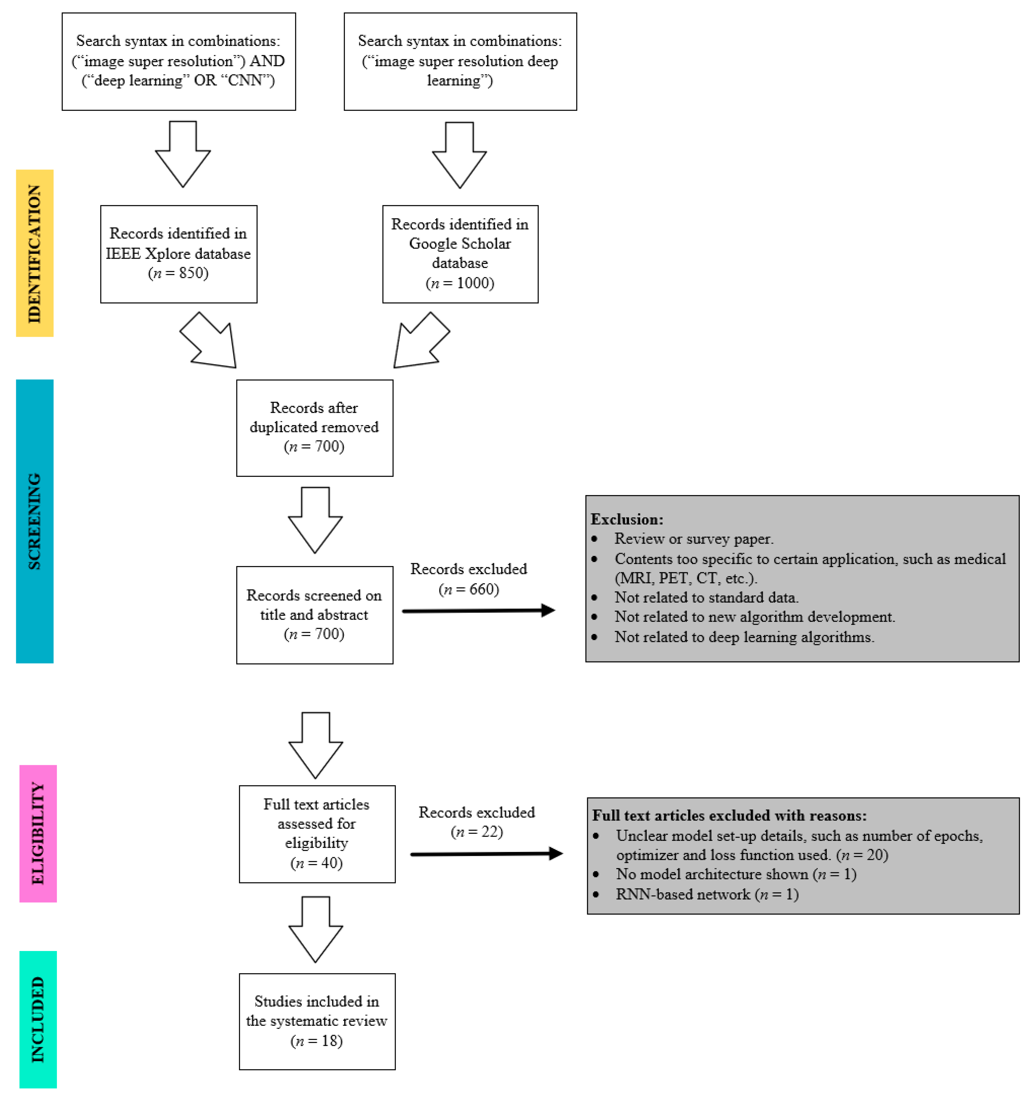
Figure 2.
SRCNN network structure (LR stands for low-resolution, HR stands for high-resolution).

Figure 3.
FSRCNN network structure.

Figure 4.
ESPCN network structure.

Figure 5.
VDSR network structure (ReLU stands for Rectifier Linear Unit).

Figure 6.
EDSR network structure.

Figure 7.
MCSR network structure.

Figure 8.
CRN network structure.

Figure 9.
ERN network structure.

Figure 10.
DRCN network structure.

Figure 11.
(a) DRRN network structure; (b) Network structure of recursive block in DRRN.

Figure 12.
GLRL network structure (PReLU stands for Parametric Rectifier Linear Unit).

Figure 13.
FGLRL network structure.

Figure 14.
DRDN network structure.

Figure 15.
SRDenseNet network structure.

Figure 16.
RDN network structure.

Figure 17.
Dilated-RDN network structure (OUnit stands for optimized unit).

Figure 18.
DSAN network structure (DSAB stands for dense space attention block).

Figure 19.
DBCN network structure.

Figure 20.
SICNN network structure.

Figure 21.
Network design strategies: (a) Linear network; (b) Residual learning; (c) Recursive learning; (d) Dense connections; (e) Dual-branch learning.
Figure 21.
Network design strategies: (a) Linear network; (b) Residual learning; (c) Recursive learning; (d) Dense connections; (e) Dual-branch learning.


Table 1.
Characteristics of datasets (modified from Wang, Chen and Hui [3]).
Table 1.
Characteristics of datasets (modified from Wang, Chen and Hui [3]).
| Datasets | Amount | Avg. Resolution | Avg Pixels | Format | Key Contents |
|---|---|---|---|---|---|
| T91 | 91 | 264 × 204 | (58,853) | PNG | car, flower, fruit, human face, etc. |
| Set5 | 5 | 313 × 336 | (113,491) | PNG | baby, bird, butterfly, head, woman |
| Set14 | 14 | 492 × 446 | (230,203) | PNG | humans, animals, insects, flowers, vegetables, comic, slides, etc. |
| DIV2K | 1000 | 1972 × 1437 | (2,793,250) | PNG | environment, flora, fauna, handmade object, people, scenery, etc. |
| BSDS100 | 100 | 432 × 370 | (154,401) | JPG | animal, building, food, landscape, people, plant, etc. |
| BSDS200 | 200 | 435 × 367 | (154,401) | JPG | animal, building, food, landscape, people, plant, etc. |
| Manga109 | 109 | 826 × 1169 | (966,111) | PNG | manga volume |
| Urban100 | 100 | 984 × 797 | (774,314) | PNG | architecture, city, structure, urban, etc. |
| ImageNet | >3.2 million | - | - | JPG | mammal, bird, fish, reptile, amphibian, vehicle, furniture, musical instrument, geological formation, tool, flower, fruit |
Table 2.
List of algorithms used in different algorithms (T stands for training datasets whereas E stands for evaluation datasets).
Table 2.
List of algorithms used in different algorithms (T stands for training datasets whereas E stands for evaluation datasets).
| Algorithms | T91 | Set5 | Set14 | DIV2K | BSDS100 | BSDS200 | Manga109 | Urban100 | ImageNet |
|---|---|---|---|---|---|---|---|---|---|
| SRCNN | T | E | E | ||||||
| FSRCNN | T | E | E | E | |||||
| ESPCN | E | E | E | T | |||||
| VDSR | T | E | E | E | T | E | |||
| EDSR | E | E | T/E | E | E | ||||
| MCSR | T/E | ||||||||
| CRN | E | E | T/E | E | E | ||||
| ERN | E | E | T/E | E | E | ||||
| DRCN | T | E | E | E | E | ||||
| DRRN | T | E | E | E | T | ||||
| GLRL | T | E | E | E | T | ||||
| DRDN | T/E | T/E | |||||||
| FGLRL | T | E | E | E | T | E | |||
| SRDenseNet | E | E | E | E | T | ||||
| RDN | E | E | T/E | E | E | E | |||
| Dilated-RDN | E | E | T | E | T | E | |||
| DSAN | E | E | T | ||||||
| DBCN | E | E | T | E | E | ||||
| SICNN | E | E | E | E | E |
Table 3.
Summary table of algorithms corresponding to their loss functions and evaluation metrics used.
Table 3.
Summary table of algorithms corresponding to their loss functions and evaluation metrics used.
| Algorithms | Loss Functions | Evaluation Metrics | |||
|---|---|---|---|---|---|
| MSE (L2) | MAE (L1) | Custom Loss | PSNR | SSIM | |
| SRCNN | √ | √ | √ | ||
| FSRCNN | √ | √ | √ | ||
| ESPCN | √ | √ | |||
| VDSR | √ | √ | √ | ||
| EDSR | √ | √ | √ | ||
| MCSR | √ | √ | √ | ||
| CRN | √ | √ | √ | ||
| ERN | √ | √ | √ | ||
| DRCN | √ | √ | √ | ||
| DRRN | √ | √ | √ | ||
| GLRL | √ | √ | √ | ||
| DRDN | √ | √ | √ | ||
| FGLRL | √ | √ | √ | ||
| SRDenseNet | √ | √ | √ | ||
| RDN | √ | √ | √ | ||
| Dilated-RDN | √ | √ | √ | ||
| DSAN | √ | √ | |||
| DBCN | √ | √ | √ | ||
| SICNN | √ | √ | √ | ||
Table 4.
Mean PSNR and SSIM for each of the algorithms. The “-” indicates no result found in the study.
Table 4.
Mean PSNR and SSIM for each of the algorithms. The “-” indicates no result found in the study.
| Scale | Algorithms | Set5 | Set14 | BSD100 | BSD200 | Urban100 | DIV2K | Manga109 | |||||||
|---|---|---|---|---|---|---|---|---|---|---|---|---|---|---|---|
| PSNR | SSIM | PSNR | SSIM | PSNR | SSIM | PSNR | SSIM | PSNR | SSIM | PSNR | SSIM | PSNR | SSIM | ||
| 2 | SRCNN | 36.66 | 0.9542 | 32.45 | 0.9067 | - | - | - | - | - | - | - | - | - | - |
| FSRCNN | 37.00 | 0.9558 | 32.63 | 0.9088 | - | - | 31.80 | 0.9074 | - | - | - | - | - | - | |
| ESPCN | - | - | - | - | - | - | - | - | - | - | - | - | - | - | |
| VDSR | 37.53 | 0.9587 | 33.03 | 0.9124 | 31.90 | 0.8960 | - | - | 30.76 | 0.9140 | - | - | - | - | |
| EDSR | 38.11 | 0.9601 | 33.92 | 0.9195 | 32.32 | 0.9013 | - | - | 32.93 | 0.9351 | 35.03 | 0.9695 | - | - | |
| MCSR | - | - | - | - | - | - | - | - | - | - | 35.09 | 0.9702 | - | - | |
| CRN | 38.17 | 0.9610 | 33.84 | 0.9203 | 32.30 | 0.9012 | - | - | 32.69 | 0.9334 | - | - | - | - | |
| ERN | 38.18 | 0.9610 | 33.88 | 0.9195 | 32.30 | 0.9011 | - | - | 32.66 | 0.9332 | - | - | - | - | |
| DRCN | 37.63 | 0.9588 | 33.04 | 0.9118 | 31.85 | 0.8942 | - | - | 30.75 | 0.9133 | - | - | - | - | |
| DRRN | 37.74 | 0.9591 | 33.23 | 0.9136 | 32.05 | 0.8973 | - | - | 31.23 | 0.9188 | - | - | - | - | |
| GLRL | 36.54 | 0.9550 | 32.56 | 0.9102 | 31.41 | 0.8890 | - | - | - | - | - | - | - | - | |
| FGLRL | 37.75 | 0.9633 | 33.11 | 0.9133 | 32.30 | 0.8842 | - | - | 29.99 | 0.9102 | - | - | - | - | |
| DRDN | - | - | - | - | - | - | - | - | - | - | - | - | - | - | |
| SRDenseNet | 32.02 | 0.8934 | 28.50 | 0.7782 | 27.53 | 0.7337 | - | - | 26.05 | 0.7819 | - | - | - | - | |
| RDN | 38.30 | 0.9616 | 34.10 | 0.9218 | 32.40 | 0.9022 | - | - | 33.09 | 0.9368 | - | - | 39.38 | 0.9784 | |
| Dilated-RDN | 38.33 | 0.9619 | 34.15 | 0.8223 | 32.44 | 0.9026 | - | - | 33.13 | 0.9372 | - | - | - | - | |
| DSAN | - | - | - | - | - | - | - | - | - | - | - | - | |||
| DBCN | 37.66 | 0.9586 | 33.15 | 0.9135 | 31.94 | 0.8961 | - | - | 31.10 | 0.9169 | - | - | - | - | |
| SICNN | 33.76 | 0.9017 | 33.23 | 0.8524 | 33.21 | 0.8309 | - | - | 32.65 | 0.8301 | - | - | 32.91 | 0.8164 | |
| 3 | SRCNN | 32.75 | 0.9090 | 29.30 | 0.8215 | - | - | - | - | - | - | - | - | - | - |
| FSRCNN | 33.16 | 0.9140 | 29.43 | 0.8242 | - | - | 28.60 | 0.8137 | - | - | - | - | - | - | |
| ESPCN | 33.13 | - | 29.49 | - | - | - | - | - | - | - | - | - | - | - | |
| VDSR | 33.66 | 0.9213 | 29.77 | 0.8314 | 28.82 | 0.7976 | - | - | 27.14 | 0.8279 | - | - | - | - | |
| EDSR | 34.65 | 0.9282 | 30.52 | 0.8462 | 29.25 | 0.8093 | - | - | 28.80 | 0.8653 | 31.26 | 0.9340 | - | - | |
| MCSR | - | - | - | - | - | - | - | - | - | - | 31.36 | 0.9359 | - | - | |
| CRN | 34.60 | 0.9286 | 30.48 | 0.8455 | 29.20 | 0.8081 | - | - | 28.62 | 0.8620 | - | - | - | - | |
| ERN | 34.62 | 0.9285 | 30.51 | 0.8450 | 29.21 | 0.8080 | - | - | 28.61 | 0.8614 | - | - | - | - | |
| DRCN | 33.82 | 0.9226 | 29.76 | 0.8311 | 28.80 | 0.7963 | - | - | 27.15 | 0.8276 | - | - | - | - | |
| DRRN | 34.03 | 0.9244 | 29.96 | 0.8349 | 28.95 | 0.8004 | - | - | 27.53 | 0.8378 | - | - | - | - | |
| GLRL | 33.09 | 0.9124 | 29.59 | 0.8705 | 28.59 | 0.7891 | - | - | - | - | - | - | - | - | |
| FGLRL | 32.95 | 0.9105 | 29.51 | 0.8325 | 28.66 | 0.7870 | - | - | 27.30 | 0.8280 | - | - | - | - | |
| DRDN | - | - | - | - | - | - | - | - | - | - | - | - | - | - | |
| SRDenseNet | - | - | - | - | - | - | - | - | - | - | - | - | - | - | |
| RDN | 34.78 | 0.9300 | 30.67 | 0.8482 | 29.33 | 0.8105 | - | - | 29.00 | 0.8683 | - | - | 34.43 | 0.9498 | |
| Dilated-RDN | 34.83 | 0.9304 | 30.68 | 0.8481 | 29.35 | 0.8109 | - | - | 29.06 | 0.8686 | - | - | - | - | |
| DSAN | 34.39 | - | 30.28 | - | - | - | - | - | - | - | - | - | - | - | |
| DBCN | 33.97 | 0.9232 | 29.95 | 0.8345 | 28.91 | 0.7993 | - | - | 27.45 | 0.8350 | - | - | - | - | |
| SICNN | 31.25 | 0.7869 | 30.97 | 0.7792 | 32.62 | 0.7902 | - | - | 31.87 | 0.8133 | - | - | 31.98 | 0.7902 | |
| 4 | SRCNN | 30.49 | 0.8628 | 27.50 | 0.7513 | - | - | - | - | - | - | - | - | - | - |
| FSRCNN | 30.71 | 0.8657 | 27.59 | 0.7535 | - | - | 26.98 | 0.7398 | - | - | - | - | - | - | |
| ESPCN | 30.90 | - | 27.73 | - | - | - | - | - | - | - | - | - | - | - | |
| VDSR | 31.35 | 0.8838 | 29.77 | 0.8314 | 27.29 | 0.7251 | - | - | 25.18 | 0.7524 | - | - | - | - | |
| EDSR | 32.46 | 0.8968 | 28.80 | 0.7876 | 27.71 | 0.7420 | - | - | 26.64 | 0.8033 | 29.25 | 0.9017 | - | - | |
| MCSR | - | - | - | - | - | - | - | - | - | - | 29.44 | 0.9020 | - | - | |
| CRN | 32.34 | 0.8971 | 28.74 | 0.7855 | 27.66 | 0.7395 | - | - | 26.44 | 0.7967 | - | - | - | - | |
| ERN | 32.39 | 0.8975 | 28.75 | 0.7853 | 27.70 | 0.7398 | - | - | 26.43 | 0.7966 | - | - | - | - | |
| DRCN | 31.53 | 0.8854 | 28.02 | 0.7670 | 27.23 | 0.7233 | - | - | 25.14 | 0.7510 | - | - | - | - | |
| DRRN | 31.68 | 0.8888 | 28.21 | 0.7720 | 27.38 | 0.7284 | - | - | 25.44 | 0.7638 | - | - | - | - | |
| GLRL | 30.37 | 0.8635 | 27.53 | 0.8102 | 26.97 | 0.7190 | - | - | - | - | - | - | |||
| FGLRL | 31.44 | 0.8846 | 28.05 | 0.7688 | 27.26 | 0.7244 | - | - | 25.13 | 0.7501 | - | - | - | - | |
| DRDN | - | - | - | - | 26.92 | - | - | - | 24.53 | - | - | - | - | - | |
| SRDenseNet | - | - | - | - | - | - | - | - | - | - | - | - | - | - | |
| RDN | 32.61 | 0.9003 | 28.92 | 0.7893 | 27.80 | 0.7434 | - | - | 26.82 | 0.8069 | - | - | 31.39 | 0.9184 | |
| Dilated-RDN | 32.64 | 0.9008 | 28.91 | 0.7892 | 27.84 | 0.7436 | - | - | 26.87 | 0.8073 | - | - | - | - | |
| DSAN | - | - | - | - | - | - | - | - | - | - | - | - | - | - | |
| DBCN | 31.78 | 0.8885 | 28.27 | 0.7733 | 27.40 | 0.7291 | - | - | 25.55 | 0.7656 | - | - | - | - | |
| SICNN | - | - | - | - | - | - | - | - | - | - | - | - | - | - | |
Table 5.
Summary table of algorithms corresponding to the upsampling module and network design strategies.
Table 5.
Summary table of algorithms corresponding to the upsampling module and network design strategies.
| Year | Algorithms | Upsampling Module | Linear Network | Residual Learning | Recursive Learning | Dense Connection | Dual-branch Learning |
|---|---|---|---|---|---|---|---|
| 2014 | SRCNN [24] | Bicubic | √ | ||||
| 2016 | FSRCNN [27] | Deconvolution | √ | ||||
| 2016 | ESPCN [43] | Sub-pixel | √ | ||||
| 2016 | VDSR [28] | Bicubic | √ | ||||
| 2017 | EDSR [37] | Sub-pixel | √ | ||||
| 2018 | MCSR [38] | Sub-pixel | √ | ||||
| 2021 | CRN [39] | Sub-pixel | √ | ||||
| 2021 | ERN [39] | Sub-pixel | √ | ||||
| 2016 | DRCN [29] | Bicubic | √ | √ | |||
| 2017 | DRRN [30] | Bicubic | √ | √ | |||
| 2019 | GLRL [31] | Bicubic | √ | √ | |||
| 2019 | DRDN [32] | Bicubic | √ | √ | |||
| 2020 | FGLRL [33] | Deconvolution | √ | √ | |||
| 2017 | SRDenseNet [44] | Deconvolution | √ | ||||
| 2018 | RDN [40] | Sub-pixel | √ | √ | |||
| 2019 | Dilated-RDN [35] | Bicubic | √ | √ | |||
| 2020 | DSAN [41] | Sub-pixel | √ | √ | |||
| 2019 | DBCN [42] | Bicubic + Deconvolution | √ | √ | |||
| 2020 | SICNN [50] | Bicubic + Deconvolution | √ | √ |
‘+’ indicated the combination particular module used.
Table 6.
Advantage and disadvantage of each algorithm.
| Algorithms | Advantages | Disadvantages |
|---|---|---|
| SRCNN [24] |
|
|
| FSRCNN [27] |
|
|
| ESPCN [43] |
|
|
| VDSR [28] |
|
|
| EDSR [37] |
|
|
| MCSR [38] |
| - |
| CRN [39] |
| - |
| ERN [39] |
| - |
| DRCN [29] |
|
|
| DRRN [30] |
|
|
| GLRL [31] |
| - |
| DRDN [32] |
| - |
| FGLRL [33] |
| - |
| SRDenseNet [44] |
|
|
| RDN [40] |
|
|
| Dilated-RDN [35] |
| - |
| DSAN [41] |
| - |
| DBCN [42] |
| - |
| SICNN [50] |
| - |
Table 7.
Advantages and disadvantage of each upsampling modules and network design strategies.
| Type | Methods | Advantages | Disadvantages |
|---|---|---|---|
| Upsampling Modules | Bicubic Interpolation |
|
|
| Deconvolution |
| - | |
| Sub-pixel Convolution |
| - | |
| Network Design Strategies | Linear Network |
|
|
| Residual Learning |
| - | |
| Recursive Learning |
|
| |
| Dense Connections |
| - | |
| Dual-branch Learning |
| - |
Table 8.
List of hyperparameters required to define a deep learning model.
| Hyperparameters | Description |
|---|---|
| Epochs | The number of iterations required for model training. |
| Batch size | The number of training image used per training step. |
| Number of filters | Refers to channel quantity of the filter in a layer. |
| Filter sizes | Refers to the two-dimensional (2D) matrix size of the filter. |
| Filter strides | Defines the number moving steps of filter in the horizontal and vertical directions. |
| Network depth | The number of layers in a model. |
| Loss functions | Learning strategies used in machine learning to measure prediction error or reconstruction error. |
Publisher’s Note: MDPI stays neutral with regard to jurisdictional claims in published maps and institutional affiliations. |
© 2021 by the authors. Licensee MDPI, Basel, Switzerland. This article is an open access article distributed under the terms and conditions of the Creative Commons Attribution (CC BY) license (https://creativecommons.org/licenses/by/4.0/).
Share and Cite
MDPI and ACS Style
Ooi, Y.K.; Ibrahim, H. Deep Learning Algorithms for Single Image Super-Resolution: A Systematic Review. Electronics 2021, 10, 867. https://doi.org/10.3390/electronics10070867
AMA Style
Ooi YK, Ibrahim H. Deep Learning Algorithms for Single Image Super-Resolution: A Systematic Review. Electronics. 2021; 10(7):867. https://doi.org/10.3390/electronics10070867
Chicago/Turabian StyleOoi, Yoong Khang, and Haidi Ibrahim. 2021. "Deep Learning Algorithms for Single Image Super-Resolution: A Systematic Review" Electronics 10, no. 7: 867. https://doi.org/10.3390/electronics10070867
Note that from the first issue of 2016, this journal uses article numbers instead of page numbers. See further details here.