Alterations in Canadian Hydropower Production Potential Due to Continuation of Historical Trends in Climate Variables


Department of Building, Civil and Environmental Engineering, Concordia University, Montreal, QC H3G 1M8, Canada
*
Author to whom correspondence should be addressed.
Resources 2019, 8(4), 163; https://doi.org/10.3390/resources8040163
Submission received: 26 August 2019
/
Revised: 16 September 2019
/
Accepted: 24 September 2019
/
Published: 29 September 2019
Abstract
:The vitality, timing, and magnitude of hydropower production is driven by streamflow, which is determined by climate variables, in particular precipitation and temperature. Accordingly, changes in climate characteristics can cause alterations in hydropower production potential. This delineates a critical energy security concern, especially in places such as Canada, where recent changes in climate are substantial and hydropower production is important for both domestic use and exportation. Current Canadian assessments, however, are limited as they mainly focus on a small number of power plants across the country. In addition, they implement scenario-led top-down impact assessments that are subject to large uncertainties in climate, hydrological, and energy models. To avoid these limitations, we propose a bottom-up impact assessment based on the historical information on climatic trends and causal links between climate variables and hydropower production across political jurisdictions. Using this framework, we estimate expected monthly gain/loss in regional hydropower production potential under the continuation of historical climate trends. Our findings show that Canada’s production potential is expected to increase, although the net gain/loss is subject to significant variations across different regions. Our results suggest increasing potential in Yukon, Ontario, and Quebec but decreasing production in the North Western Territories and Nunavut, British Columbia, and Alberta.
1. Introduction
Increasing global energy demand, limiting fossil fuel resources as well as looming effects of climate change have created the urgency for looking at alternative energy resources, in particular renewable energy supplies [1]. In contrast to fossil fuels, renewable energy sources are sustainable, constantly replenished, easily convertible to electricity, and are not associated with large greenhouse gas emissions. These characteristics make renewable energy sources ideal for moving towards a carbon-free global economy [2,3]. Currently hydropower accounts for the highest proportion of renewable energy supply globally [4]. There are several countries, such as Canada, where national energy security is largely dependent on the hydropower. The majority of Canada’s hydropower facilities are located in the provinces of Quebec, British Columbia, and Ontario [5,6,7], that include the largest population and concentration of socio-economic activities. Hydropower is currently the first source of electricity supply in Canada. In 2015, hydropower supplied 95% of the electricity need in Québec, 97% in Manitoba, 95% in Newfoundland and Labrador, and 86% in British Columbia [8]. In the same year, Canada was the second largest hydroelectric exporter in the world, generating 10% of the world’s hydroelectricity exportation [9], half of which was contributed by Québec only [10].
Canada owes this massive production potential to a large network of rivers and lakes, distributed coast to coast. From the hydrological perspective, running water is the main driver of hydropower production. The seasonal, annual, and interannual characteristics of runoff, however, are largely controlled by climate variables in particular precipitation and temperature [11,12,13]. As a result, alterations in climate variables can consequently lead to changes in hydropower production potential [14,15,16]. This, in fact, is a global concern considering significant increasing trends in temperature since the mid 20th century [17,18,19] including in Canada [20,21,22,23], where the rate of warming is nearly twice of the global average [24]. Such significant warmings are mainly attributed to the increase in the concentration of greenhouse gases and can cause major changes in other climate variables such as precipitation and evaporation [25,26,27]. Such changes, in turn, alter natural runoff regimes [28,29] with large temporal and spatial differences [19,30,31,32]. This is particularly the case for precipitation [33,34,35], as not only the amount, but also the form of precipitation can also change due to warming [36,37].
The effects of warming are expected to be more intensified under future conditions [38,39,40,41,42] and can largely affect hydropower generation potential globally, regionally, and locally [43,44]. Projections of future runoff show significant decreases in mid-latitudes and some dry tropics by the end the 21st century, which can jeopardize hydropower production potential in southern Europe, northern Africa as well as the Middle East [45,46,47,48,49]. Analyses of hydropower production potential under warming climate in northern countries, such as Canada, highlight the opportunity for increasing power generation potential due to increased glacial melts, which act as additional sources of runoff [50,51,52]. Having said that, climate change-induced shifts in timing of the runoff can offset the effect of increasing the annual runoff volume [53,54,55,56], as the surplus runoff may translate to unproductive spill, depending on the available reservoir storage and/or the turbine capacity [57,58,59].
Current studies portray an overall increase in Canadian hydropower production potential, with increasing and decreasing trends in northern and southern parts of the country, respectively [60,61,62]. These findings however are quite uncertain. Primarily, climate impacts on hydropower generation often involves multiple intermediate physical processes that are not fully known, particularly at larger scales [63]. In addition, climate impacts on runoff can transcend across different temporal scales [43], and are subject to large spatial differences [16,64,65]. Apart from inherent complexity in physical processes that determine hydropower production potential, methodological frameworks, with which the climate change impacts are assessed, are still incomplete. For instance, current studies only focus on a small number of hydropower plants across the large Canadian landmass; and therefore, extrapolation of the results to political jurisdictions, where management decisions are made, is not readily possible. In addition, the majority of impact assessments are built upon the IPCC-endorsed top-down and scenario-led impact assessment framework [25], which includes a cascade use of climate along with hydrological and energy simulation models. These models are still limited. For instance, climate models still struggle to accurately represent the historical climate, particularly with respect to precipitation [37,66,67]. Furthermore, hydrological models that convert the climate forcing to streamflow sequences have major issues in their structures, parameterizations, and data support [68,69,70,71]. Most importantly, climate change impacts can be largely offset or amplified by human intervention in land and water management [72,73,74], however current hydrological models are limited in terms of representing human activities within hydrological cycle [75,76]. Finally, energy simulation models, with which power production is estimated based on water availability and socio-economic variables, can be another source of uncertainty. A study in Canada showed that by changing the energy simulation model only, the estimated magnitude of change in hydropower production can differ up to 50% [77]. The total uncertainty can be therefore substantially large and can hinder their application in real-world decision making processes [78].
An alternative approach to top-down impact assessments is to use historical data or synthetic hydroclimatic scenarios as a basis for doing “stress-tests”. Such assessments, which are particularly useful for management purposes, are geared toward representing critical thresholds under which the system under consideration becomes vulnerable. Applications of bottom-up impact assessments have been growing recently [79,80], including in the hydropower domain [11,81,82,83,84,85]. Here, we aim at developing a fully bottom-up, empirically-based impact assessment framework to provide a synoptic look at the impacts of climate change on hydropower production across political jurisdictions in Canada. We recognize that current assessments (1) may not be relevant at larger scales, particularly across political jurisdictions where management decisions are made; and (2) are subject to large uncertainties due to limitations in current modeling technology that support impact assessment. To avoid these gaps, we focus on understanding empirical trends in regional climate variables, as well as dependency and causal links between regional climate variables and hydropower production. On the one hand, regional climate trends can provide a set of plausible scenarios for changing climate conditions at the larger scales. On the other hand, understanding causal links between climate variables and hydropower production can provide a basis for developing data-driven predictive tools, with which the expected gain/loss in monthly hydropower production across Canadian jurisdictions can be assessed. Section 2 provides more details on the rationale and assessment procedure used in this study. Section 3 introduces the data availability for historical monthly hydropower generation in Canada along with climate data used to compile regional climate variables across Canadian jurisdictions. Section 4 introduces the methods used for upscaling climate data, quantifying climate trends, understanding the dependency and casualty between climate and hydropower generation, as well as developing predictive models for simulating monthly regional hydropower production. Section 5 presents and discusses our results. Section 6 applies the findings towards assessing the sensitivity of regional hydropower production to continuation of the historical climate trends. Finally, Section 7 concludes this study and provides some further remarks.
2. Rationale and Assumptions
We aim at introducing a fully bottom-up scheme that can reveal expected change in hydropower production potential, if historical trends in climate variables continue in the future. Figure 1 shows a schematic view to the proposed framework. The procedure starts with estimating regional climate variables based on a number of in situ climate measurements. We then use a statistical trend test to investigate monotonic changes in regional climate variables across monthly, seasonal, and annual scales. In parallel, we use two other statistical tests to assess the dependency and casual links between lagged climate variables and hydropower production. After understanding specific climatic causes of hydropower generation at each political region, different competing hypotheses for simulating monthly hydropower generation are formed and tested to infer the best predictive model for impact assessment. We then plug the historical trends in regional climate variables to the non-falsified predictive models to portray what would be the historical hydropower production, if historical trends continue as-is in the future. Using this framework, the sensitivity of hydropower production to continuation of climatic trends can be assessed without using climate, hydrological, and energy simulation models.
Our proposed framework is based on two key assumptions. Most importantly, we use the observed trends in climate variables as a basis to perform the impact assessment. Accordingly, our assessment aims at understanding “what would be the change in the historical hydropower production, if current trends in climate variables continue in future”. This implies that no other variable, e.g., generation capacity, demand-production balance, etc., is changed. We recognize that the hydropower production is also driven by the electricity demand, for which the drivers of change can go well beyond the climate variables at the region where hydropower is produced. As a result, our proposed assessment essentially addresses the change in “hydropower production potential” rather than actual change in hydropower production itself. Second, our assessment essentially considers each political region as a standalone hydropower production unit, in which the fluctuations around the expected production can be described by the fluctuations in relevant climate variables at the same regional scale. Due to this conceptualization, we can consider developing a set of predictive Box-Jenkins models, with which the monthly hydropower productions at each political jurisdictions can be described as a set of autoregressive functions with inputs from corresponding regional climate variables across a range of temporal scales. This assumption, however, is not taken for granted and will be tested rigorously through a comprehensive setup/falsification procedure to evaluate the credibility of the predictive models and accordingly the assessments made.
3. Data Support
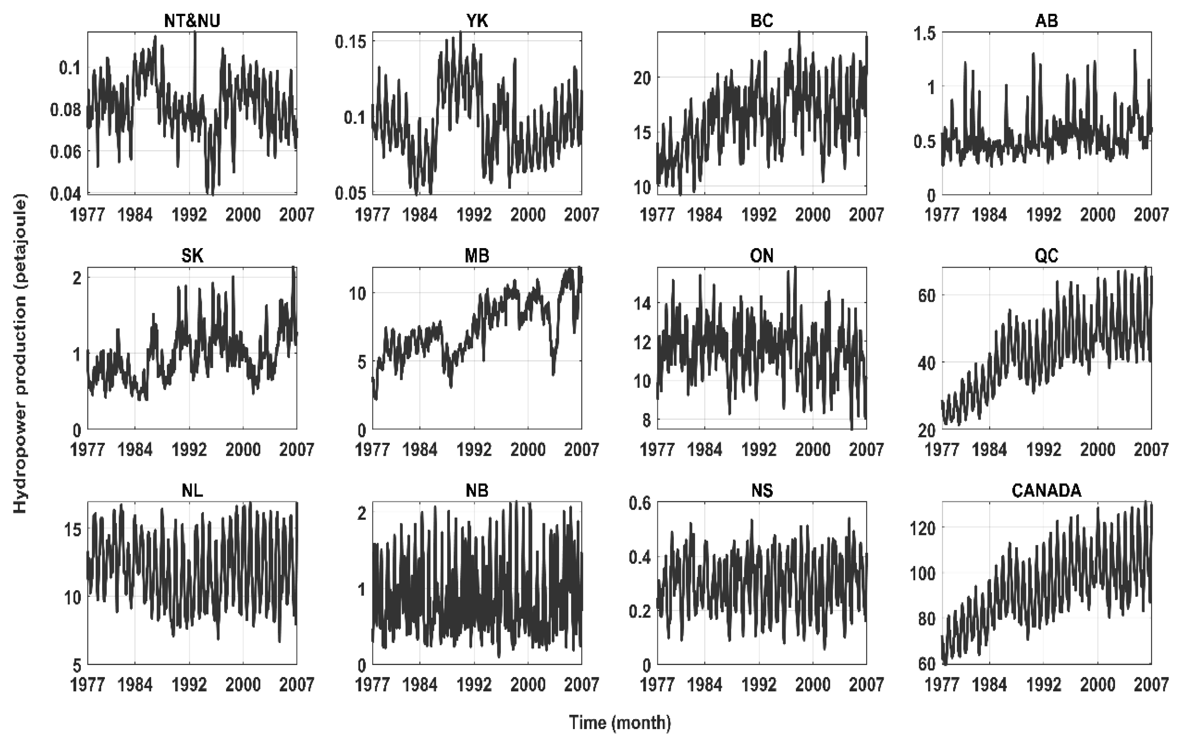
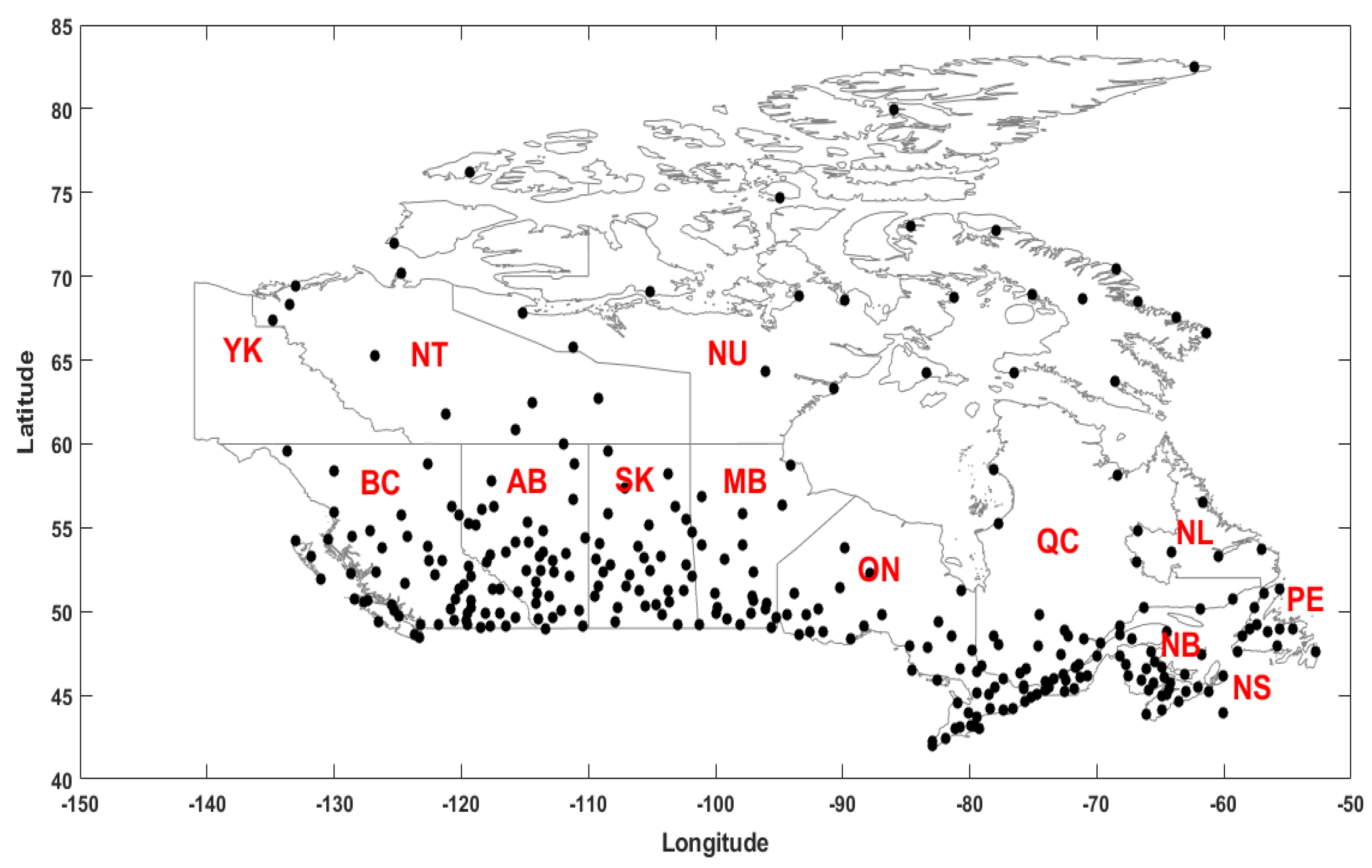
The data related to monthly hydropower production across Canadian jurisdictions, covering the period of January 1977 to December 2007, are publicly available through Statistics Canada’s key socioeconomic database (CANSIM; http://www5.statcan.gc.ca/cansim). It should be noted that the data for Nanuvat and Northwest Territories are given as one regional unit and there are no data for Prince Edward Island due to insignificant hydropower production. Figure A1 in Appendix shows the monthly time series of hydropower production across Canadian political regions.
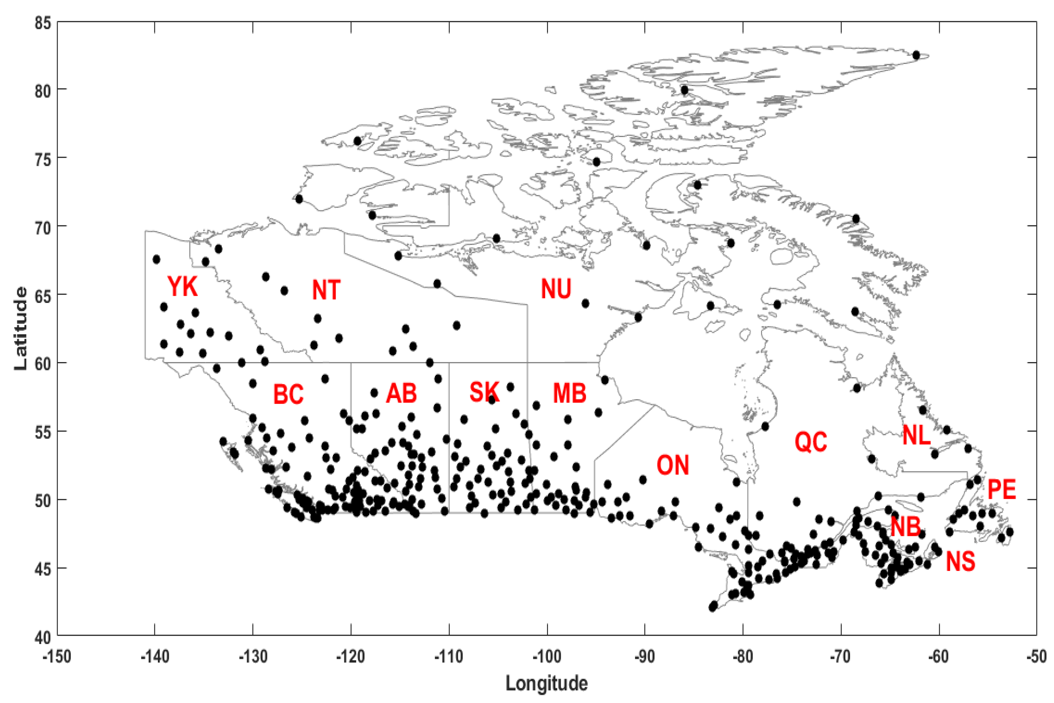
The historical climate data are taken from the APC2 archive, developed by the Environment and Climate Change Canada. The data have been already used for addressing climate change impacts in Canada [86,87,88] and is publicly available at https://www.canada.ca/en/environment-climate-change/services/climate-change/science-research-data/climate-trends-variability/adjusted-homogenized-canadian-data.html. We consider total monthly values of precipitation, rainfall, and snowfall along with monthly mean temperature across a large number of Canadian climate stations that have data during the period of 1977 to 2007. Precipitation data are available at daily scale and include adjusted rain and snowfall amounts across 450 climate stations. For each station, we aggregate the daily data to come up with monthly estimates. The stations with more than 15% of missing data are discarded from our analyses. This results into selecting 379 precipitation stations. The distribution of selected precipitation stations are shown in Figure A2 in the Appendix. Similar to precipitation, the daily temperature data are aggregated into mean monthly estimates and stations with more than 15% of missing data during 1977 to 2007 are discarded from the analysis. Accordingly, 308 stations from the total of 338 stations are selected. The distribution of the selected stations are shown in Figure A3 in Appendix.
4. Methodology
4.1. Upscaling Climate Variables
There is a scale mismatch between local climate and regional hydropower data. Accordingly, we upscale the available monthly climate data at each Canadian jurisdiction to come up with regional estimates of climate variables. To do so, we use a gridding scheme, proposed by Han et al. [89]. The algorithm divides the whole landmass into a finite number of grids and calculates the weights of association of each station to each grid. The grid size can be predetermined based on the total area and total number of stations, respectively. Weighting is based on the inverse of squared Euclidian distance between the centre of the grid and each station, i.e., closer stations have a higher weight compared to distant stations. After the weights of all stations to each grid is assigned, the grid-wide estimate for the considered climate variable can be calculated as the weighted average of all stations in the considered region. Accordingly, the regional climate variable can be estimated using the arithmetic mean of all grids in that region—see [89] for more details.
4.2. Quantifying Trends in Regional Climate Variables
The analysis of trend involves detecting the signal of a monotonic temporal change in a particular climate variable and includes quantifying direction, magnitude, and significance of the change [90]. Here, we apply the Mann-Kendall trend test [91,92]. The method is non-parametric, and therefore, does not require any assumption about statistical properties of data [92]. This makes the test particularly suitable for detecting monotonic changes in hydroclimatic data [93,94,95,96,97]. The null hypothesis of the Mann-Kendall test is the existence of no trend. The rejection of the null hypothesis requires a significant upward or downward slope. Like any other formal statistical test, the significance can be objectively inspected using the p-value. Here, we consider the p-value of 0.05 as the threshold for distinguishing between significant and insignificant trends. The slope is often calculated by the Sen’s slope, which is a robust estimation of the linear trend [98]. The advantages of using Sen’s slope estimator is its insensitivity to extreme values that can dampened or exaggerate the true trend. Due to the different scales and/or dimension of climate variables, the trend test is performed on the anomaly of the time series, so that the results from various regions and/or variables can be comparable. The anomaly can be calculated as the following:
where and are the transferred and raw data; and and σ are the mean and standard deviation of the raw data.
4.3. Analysing Dependency between Hydropower Production and Climate Variables
The analysis of dependency aims at understanding the statistical association between a pair of random variables and is a commonly-used inference in hydrology and water resource management [99,100,101]. Here, we used Kendall’s tau [102], which is a scaled and non-parametric measure for evaluating the degree of similarity between two sets of random variables [103]. The absolute value of the Kendall’s tau shows the magnitude and its sign indicates the direction, where one is the complete positive dependence, zero is no dependence, and −1 is the complete negative dependence. Again, we consider p-value of 0.05 as the threshold for distinguishing between significant and insignificant test results. We consider analyzing the dependency between the hydropower and lagged climate for lags between zero to 11 months. This is due to the fact that hydrological processes that affect runoff generation have annual recurrence and therefore the considered range can fully reveal the intra-annual links between climate drivers and hydropower production at the same regional scale.
4.4. Diagnosing Climate Causes of Hydropower Production across Canadian Jurisdictions
Statistical dependency between climate variables and hydropower production does not necessarily imply causality [104]. Testing causality requires an exclusive statistical framework to quantify the significance of how occurrence of causes (here regional monthly climate variables) makes changes in the effect (here monthly regional hydropower generation). One of the most intuitive explanations of causal relation between two time series was introduced by Wiene [105] and later formalized by Granger in 1969 as a formal statistical test, known as “Granger causality test” [106]. The test has been used in several milestone hydroclimatological studies. Most importantly, in understanding the causal effect of CO2 on the global warming [107,108], El Nino’s southern oscillation on the Indian monsoon [109], sea surface temperature on the northern Atlantic oscillation [110], and feedback effects between land cover on the local climate [111,112].
Granger causality works based on the concept of prediction using linear autoregressive models with or without considering exogenous variables [106]. The test is built upon two main assumptions: First, the cause is always prior to the effect in terms of the occurrence. Second, knowing the cause improves the prediction of the effect. To better understand the concept of Granger’s causality test, assume and are two separate time series. If we are better able to predict by using the past value of both and rather than only using the value of , then is the Granger cause of [113]. This means that the past values of have additional information to help predicting with more accuracy. The procedure of Granger causality starts from modeling a particular effect (here hydropower) only based on its own past values using a simple autoregressive model (hereafter AR). Considering the AR with the order , with can be calculated as:
where is the predicted time series, is the prediction error, and are model coefficients in the AR model. The order can be empirically found by analyzing the autocorrelation structure of . Considering the AR model, the quality of predicting depends only on the past values of . The prediction error of the AR model can be formally assessed with the unbiased variance of prediction error, calculated as the following:
here, is the length of the time series, and is the sum of squared errors in the AR model. Alternatively, an autoregressive model with an exogenous variable (hereafter ARX) can be considered with the same order to simulate by considering both values of and [106]:
where is the predicted time series, is the prediction error, and are the coefficients of the ARX model, associated with the past values of both effect (here hydropower production) and cause (here one climate variable), respectively. The variance of the prediction error of for the ARX model can be estimated as:
where the prediction error of depends on the past values of both the effect and the cause. According to the definition of Granger causality, if the prediction error of ARX model is smaller than the prediction error of the AR model, then it can be inferred that is a Granger cause of [106]. To objectively compare the prediction errors, the complexity of AR and ARX models should be also considered, given the fact that they contain different number of parameters. For this purpose, the Bayesian information criterion (BIC) can be used [114]:
where is the sample size, is the sum of squared residuals, and is the number of free parameters in the model. The lower the BIC is, the more efficient the model.
4.5. Developing Predictive Models for Regional Hydropower Production
By knowing the climatic causes of hydropower production at each political region, different predictive models can be set up for simulating regional hydropower production by combining past values of hydropower production as well as climatic causes. To avoid dimensional inconsistencies and scaling issues, regional hydropower and climate time series should be first mapped into a homogeneous space. We considered standardizing data within 0.1 and 0.9 to allow extrapolation capability in both predictors and predict beyond the observed range [115,116]. Here, four schemes for setting up the autoregressive models are considered that differ from one another in terms of how climate causes are considered within the formulation of the autoregressive models. In Scheme A, only the dominant climate cause of hydropower generation at each time lag is considered. The dominant climate cause at each time step is the climate variable that makes the highest improvement in the prediction of hydropower production. Scheme B is similar to Scheme A, but instead of considering only the dominant climate causes at each time step, their corresponding values at the previous time steps are also considered. In Scheme C, all climatic causes of hydropower at each previous time lag are considered. Scheme D is similar to Scheme B but apart from the dominant climate cause at each time step, all climate causes are considered. Table 1 summarizes the four setups considered for developing predictive models for simulating hydropower production at each region. In terms of complexity, Scheme A resembles the most parsimonious model and Scheme D is the most parametrically-complex representation. For each region, several competing hypotheses for simulating hydropower generation are formed using the four schemes and considering all possible time lags from one month to the critical number of time lags, after which there is no trace of climatic causes in the hydropower time series.
To systematically develop, compare, and falsify predictive models at each region, the available data is divided into two parts, related to calibration and validation of predictive models. For this, we used the first 80% of the data for calibration and the last 20% for validation. During calibration, the parameters of the predictive models are identified using the least square estimator. Using the extracted parameters, the monthly hydropower production is simulated for the remaining 20% of the data. Each modeling hypothesis is utilized in two different simulation modes, related to offline and online simulations. Offline simulation mode refers to the simulation condition, in which current hydropower generation is simulated using observed hydropower production as well as climate causes in the previous time step. In the online mode, in contrast, past hydropower productions are obtained from past simulation time steps and therefore simulation errors can transcend from one time step to the next simulation time steps. The performance of the developed models during the training and testing periods are inspected using the BIC, root mean square error (RMSE) and the coefficient of determination . For each region, the modeling alternative that has the best online performance based on R2 in the testing period is chosen as the non-falsified predictive model, which can be further used for impact assessment.
5. Results and Discussion
5.1. Validating Upscaled Climate Data
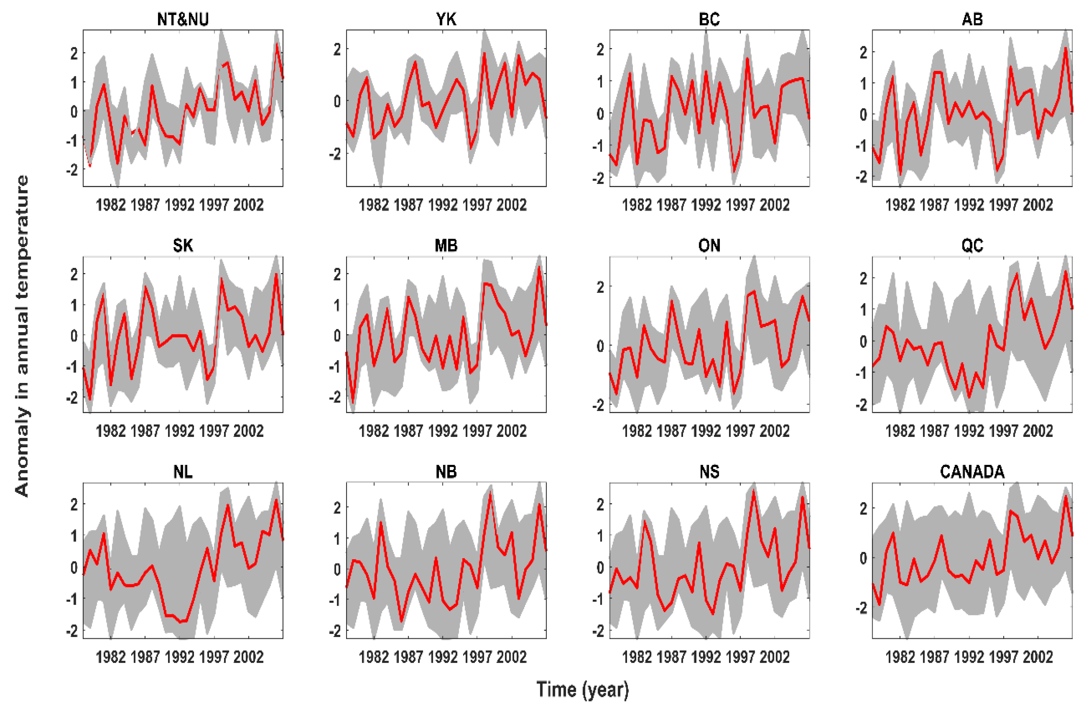
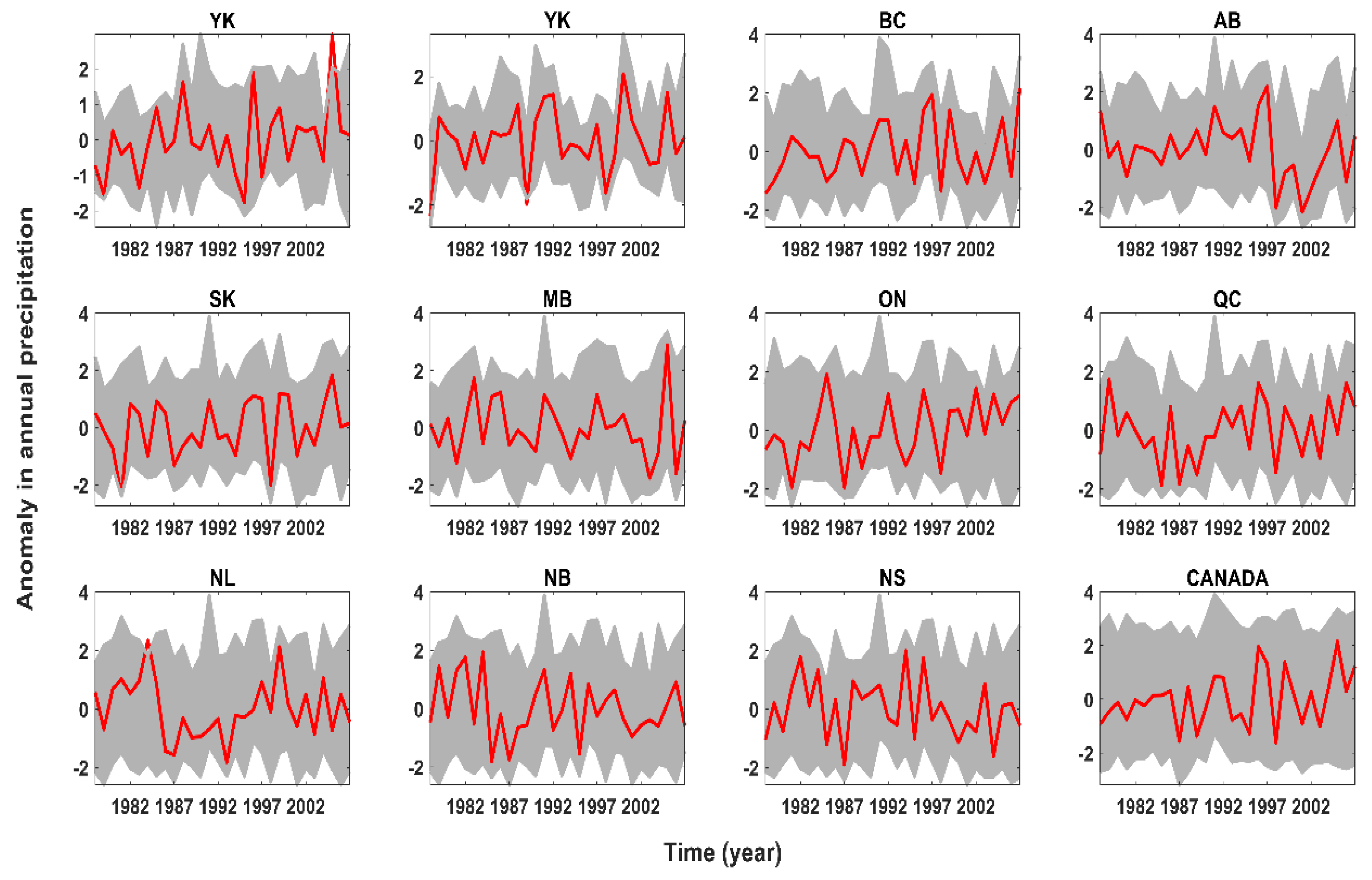
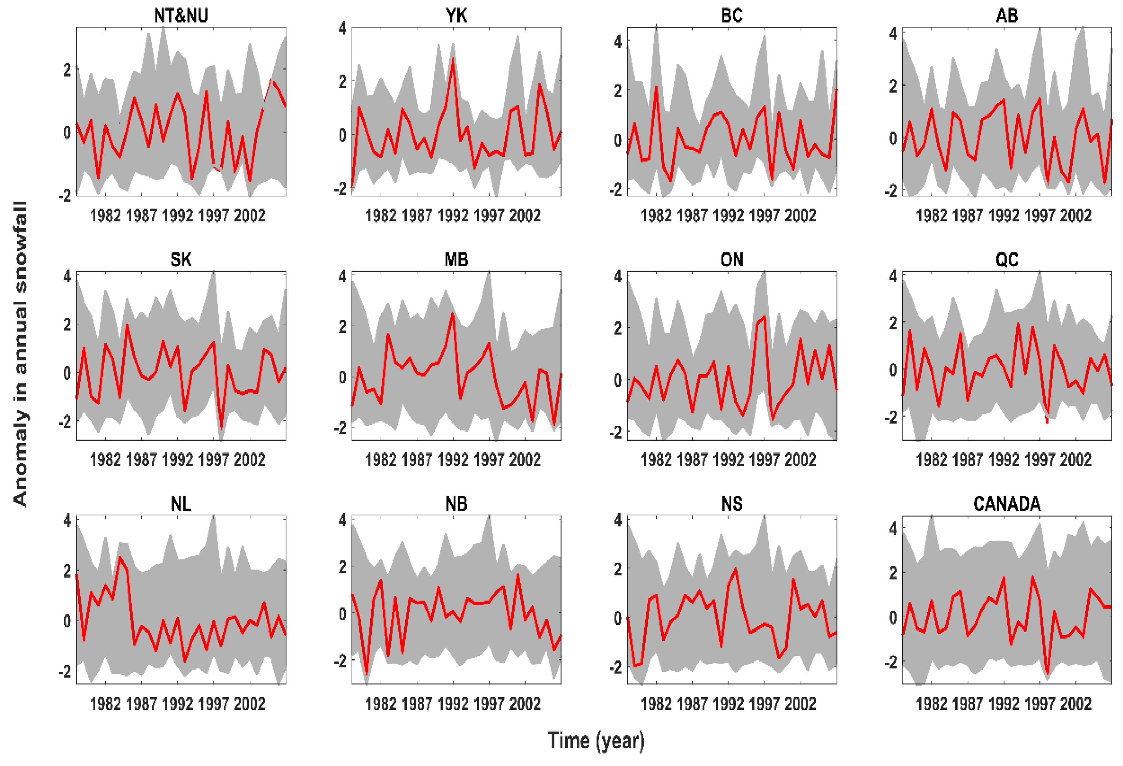
Before using the regional climate data for further analyses, we evaluate the skills of upscaled climate variables in capturing spatiotemporal variability at each region. For this purpose, we calculate the anomalies in annual climate variables across all stations located in a given region and compare them with the anomaly in corresponding upscaled regional climate variables—see Figure A4, Figure A5, Figure A6 and Figure A7 in Appendix for temperature, precipitation, snowfall, and rainfall, respectively. In all regions and for all climate variables, the upscaled climate variables are within the empirical variability observed collectively in the in situ data. We also look at how trends in anomalies of climate variables across climate stations can be maintained by corresponding upscaled climate variables. The results are presented in Figure A8 in the Appendix for temperature, precipitation, snowfall, and rainfall, respectively. The results confirm that the trends of upscaled climate anomalies are within the empirical range in all cases, expect for Nunavut (NU) and Northwest Territories (NT) for mean temperature. This is due to sparse networks of stations distributed unevenly within this large region.
5.2. Trends in Regional Climate Variables
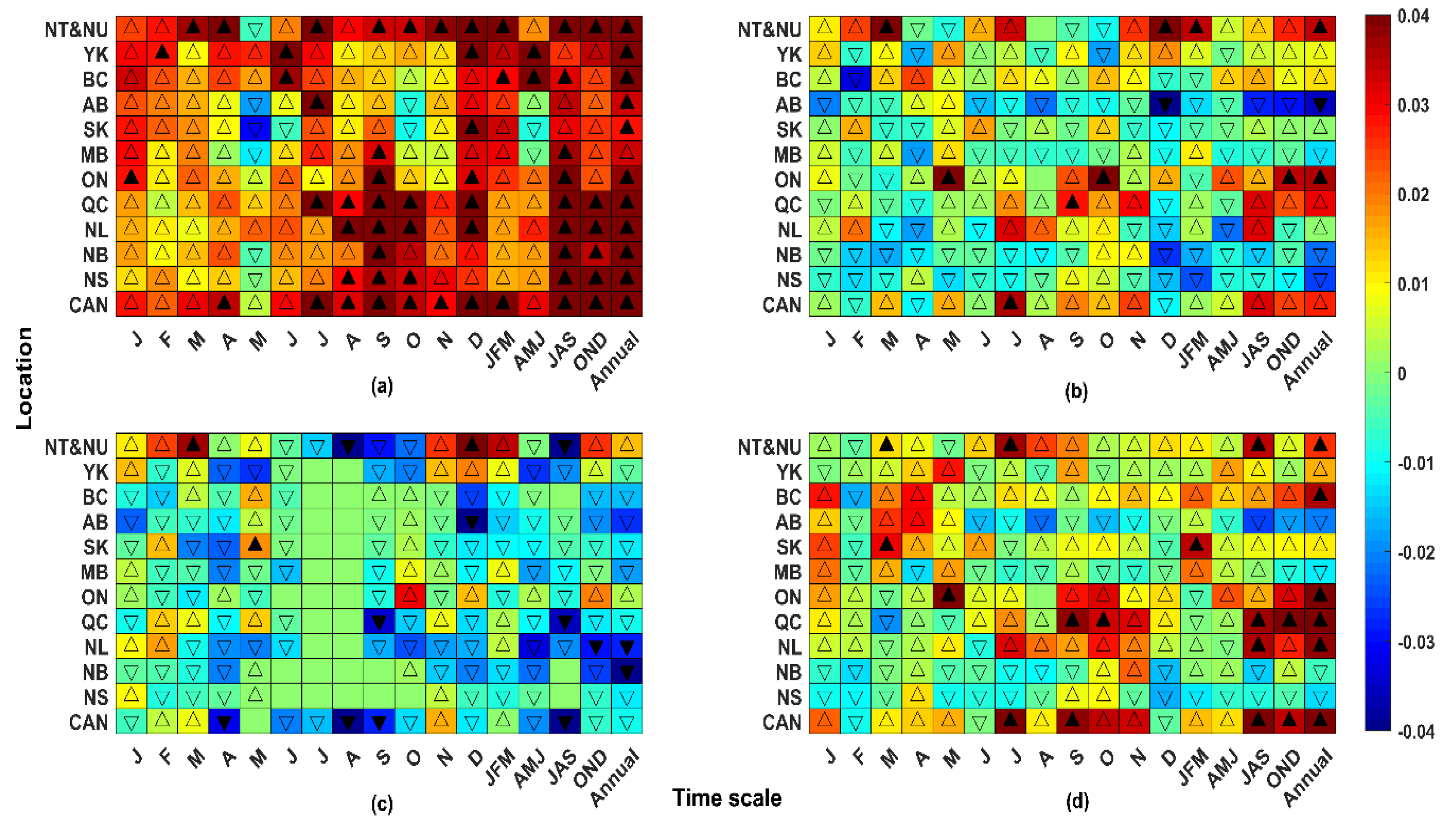
We apply the Mann-Kendall trend test to the anomalies of upscaled climate variables at monthly, seasonal, and annual scales. The results are illustrated in Figure 2 using a set of standardized heat maps, in which x-axis indicates, monthly, seasonal, and annual time scales, respectively from left to right. Political regions are shown in the y-axis and are ordered based on their location. From top to bottom, it starts with northern regions, then goes from west to east and finally shows Canada as a whole. In each cell, the magnitude of trend in anomalies of climate variables are color coded based on a unified scheme to allow comparison between different variables. Upside and downside triangles indicate positive and negative trend, respectively. Significant trends at 95% confidence limit are shown by filled triangles.
With respect to the mean temperature, the majority of trends are positive across considered temporal and spatial scales. In addition, all significant trends are positive showing that Canada is extensively warming. During the winter of 1977 to 2007, all provinces experienced an increase in mean temperature, with significant increases in NU and NT, British Columbia (BC), and Canada as a whole. During spring, trends are significant and positive in Yukon (YK) and BC; but they are insignificant and negative in Saskatchewan (SK) and Manitoba (MB), and insignificant and positive in other regions. The mean temperature increased during the summer across all provinces. The captured trends are significant in all provinces except in YK, Alberta (AB) and SK. During the study period of 1977 to 2007, mean temperature in the fall increased across all regions. These increasing trends are significant in NU and NT, Quebec (QC), and the Atlantic provinces. In the annual scale, significant and positive trends are captured in all regions except in MB, which is still positive but insignificant. Such warmings can cause significant alteration in hydrological processes that affect runoff generation.
Regarding monthly precipitation, trends can be divergent across various spatial and temporal scales. For instance, in the northern regions, trends are positive in January, March, June, July, November, and December but negative in April and October. In the western provinces, precipitation increased mainly in January and May, but decreased in February, July, and December. The trends are also positive in the eastern provinces through May to July, as well as September to November. In terms of seasonal trends, northern regions experienced increments in total precipitation during the winter. The trend was also positive in MB, QC, and Newfoundland (NL), but the significant trends have only occurred in NU and NT. BC, AB, SK, Ontario (ON), New Brunswick (NB), and Nova Scotia (NS) experienced insignificant negative trends in total precipitation. In spring, positive trends are captured in NU and NT, BC, and ON, however, other regions show insignificant negative trends. During the summer season, most regions experienced insignificant increments in total precipitation except in AB, MB, NB, and NS. Total precipitation has increased across the northern regions, BC, SK, as well eastern provinces but decreased in other regions during the fall. In the annual scale, northern regions experienced increments in total precipitation, which is significant in NU and NT. In AB, annual precipitation significantly decreased, while ON experienced a significant increase.
Similar to precipitation, trends in snowfall show different patterns across various temporal and spatial scales. In general, during the winter, snowfall increased insignificantly in northern regions; however, it decreased along western, eastern, and Atlantic Canada except in MB, QC, and NL. Having said that both negative and positive trends are insignificant. In spring, all regions show negative trends in snowfall except in ON, which shows an insignificant positive trend. During the summer, northern regions show negative trends, which is significant in NU and NT. The amount of snowfall decreased during fall across the whole country except in the northern regions and ON. Considering the annual scale, the snowfall insignificantly increased in NU and NT, but decreased over western, eastern, and Atlantic provinces except in ON. The negative trends are found to be significant in NL and NB. In general, our study confirms the overall decrease in snowfall throughout Canadian regions. With respect to rainfall, in contrast, it seems that positive events outnumber negative trends and increasing trends are stronger in summer and fall. Total rainfall has increased across the country except in ON, QC, and NS during the winter. Having said that, the only significant positive trend captured in SK. Total rainfall increased across Canada during the spring except in AB, NL and NS; however, all trends are insignificant. During the summer, all regions experienced increments in rainfall except AB, NB, and NS. The captured increasing trends are significant in NU and NT, QC, and NL. During the fall, trends in rainfall are positive in all provinces except in AB, MB, and NS. These trends are significant over QC and Canada as a whole. In the annual scale, trends are positive in northern regions, which is significant in NU and NT. In western provinces, BC and SK experienced increments in rainfall and the trend is significant in BC. Decreasing trends however are observed in AB and MB. At the annual scale, rainfall has increased significantly in eastern provinces; however, across Atlantic provinces, only NL has experienced a significant increase in rainfall.
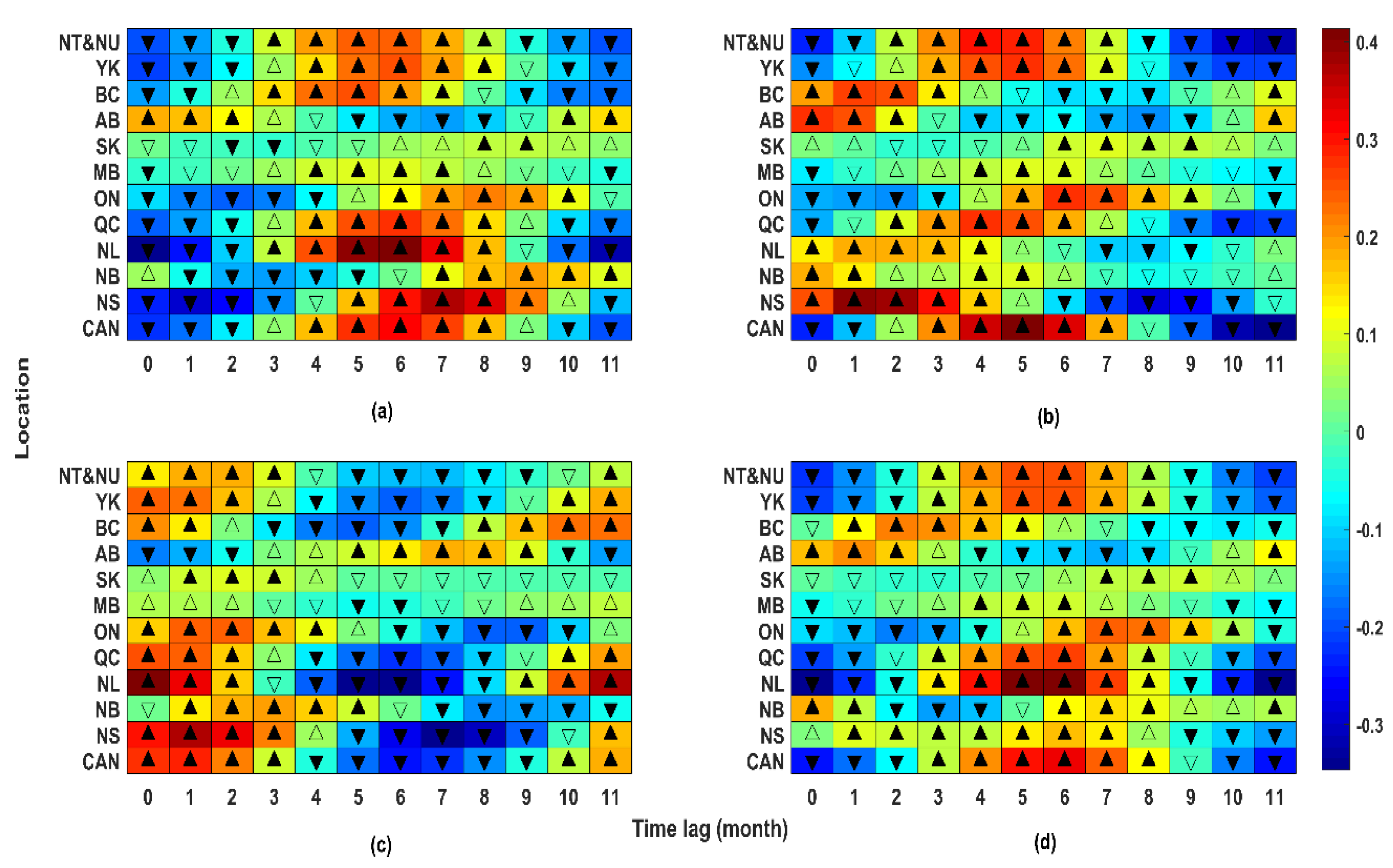
5.3. Regional Dependencies between Climate Variables and Hydropower Production
Similar to the analyses of trend, the results of dependency analyses between lagged climate variables and hydropower production are summarized in four heat maps—see Figure 3. Heat maps in Figure 3 are slightly different from those presented in Figure 2 as the x-axis refers to the lagged climate variables sorted from zero to 11 months. Positive and negative dependencies are shown with upward and downward triangles. In addition, significant dependencies (p-values ≤ 0.05) are shown with filled triangles. With respect to temperature, except in AB, the relation between mean temperature and hydropower generation is significantly negative in first months. After few months, the negative dependency becomes positive. This observation excludes SK, in which the dependence is negligible. This pattern in inverted in AB, which can be referred to the particular runoff generation/hydropower production dynamic in this province, where the majority of power plants are located at the eastern slopes of Rocky Mountains, which receives a large annual snow pack over a small region and therefore the annual snowmelt is often extensive and fast.
Few strong patterns can be seen for dependency between precipitation and hydropower generation, which can reveal important natural and anthropogenic mechanisms behind hydropower generation across Canadian regions. In the first few lags, there are two distinct patterns showing different effects of total precipitation on hydropower generation in AB, BC as well as Atlantic provinces (i.e., positive effect), versus what is observed in northern and eastern Canada as well MB (i.e., negative effect). First it should be noted that the mechanism of runoff generation in mountainous BC and AB is largely different from those in QC and ON, in which negative dependence within the first time lags can be referred to unproductive spillage [117]. A historical example in QC includes additional release ordered by Hydro-Quebec in 1996 to preserve the integrity of reservoirs against heavy rainfall. This spillage did not add to power generation as it was beyond the turbine capacity [118]. The negative dependency, however, change to positive after few months except in mountainous provinces. SK resembles an outlier case, as the hydropower generation in this province is not significantly dependent on its own precipitation in most of the time lags. MB also has a negligible dependency in comparison with other provinces, meaning that the power generation in MB and SK are not dependent to the precipitation poured over their own territory. This is intuitively appealing as water in SK and MB is mainly contributed from upstream province of AB [119].
With respect to snowfall, all provinces except AB and NB show a positive dependency between snowfall and hydropower production in the first months. These dependencies are statistically significant in the majority of regions, excluding MB. The lack of significant dependency between snowfall and hydropower production in this region can be traced back to the fact that majority of water availability for hydropower production in MB is contributed from the mountainous headwaters in AB. As the lag between snowfall and hydropower production increases, positive dependencies turn to negative. The dependency between rainfall and hydropower production, however, is rather different. All regions, except AB, NB and NS, have negative short-term dependencies with rainfall. The negative rainfall dependency is relatively longer and more significant in ON. The dependency is also significantly negative in Canada for the first three months, and then changes to significantly positive. Similar to the hydropower and precipitation dependency, this can be referred to the impact of storage and the fact that immediate rainfall can go to unproductive spillage, if the reservoir storage is already full.
5.4. Climatic Causes of Hydropower Production across Canadian Jurisdictions
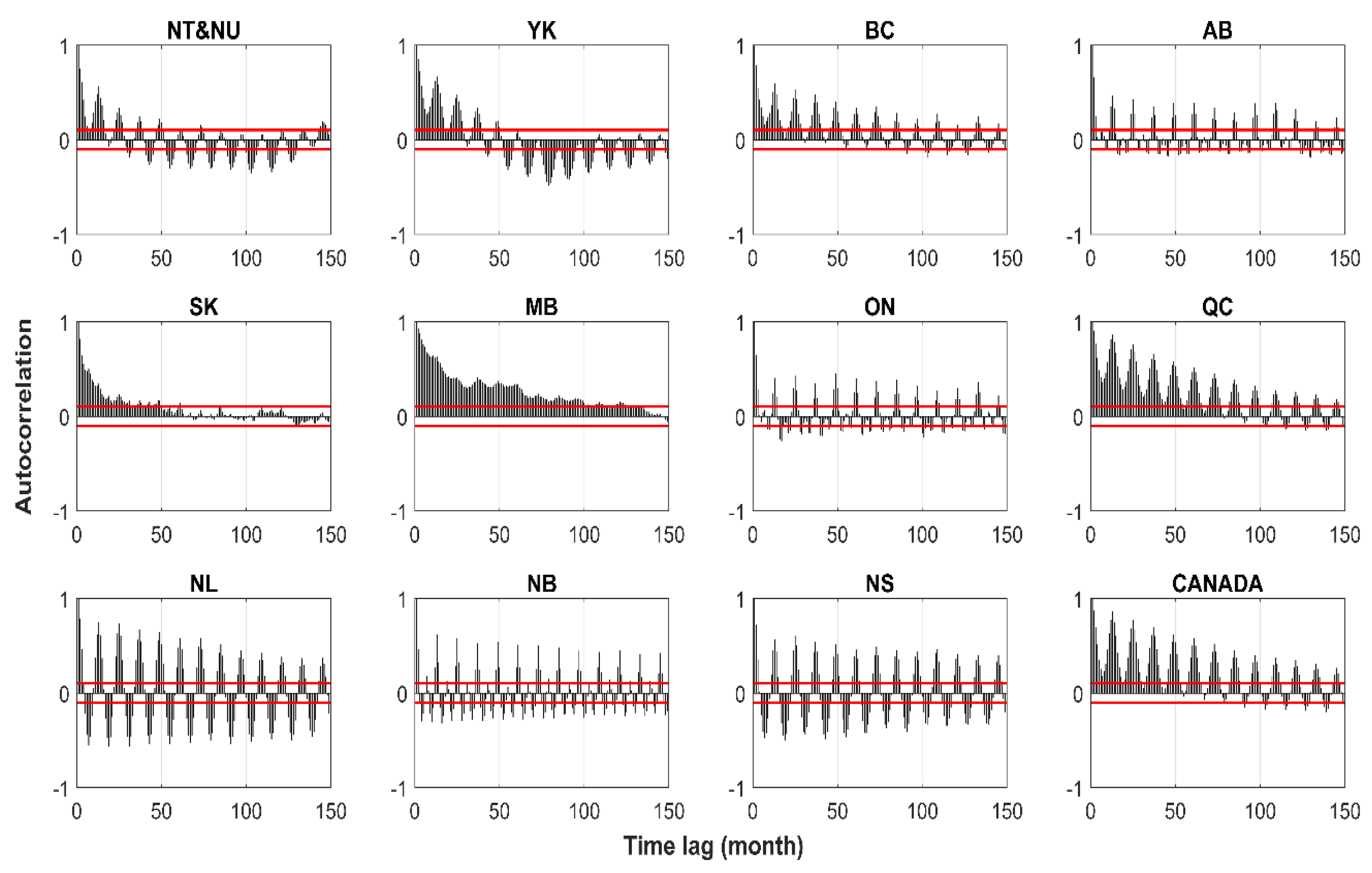
Identifying climatic causes of hydropower production at each region is based on the intercomparison between a wide range of AR and ARX models that represent monthly hydropower production. The model development starts with analyzing the autocorrelation structure within monthly regional hydropower production, which reveals to what extent hydropower generation is dependent to its previous values. Potentially, all lags up to the first break in significance of autocorrelation (i.e., first occasion where p-value goes above 0.05) can be considered for forming AR models. Our analyses show that autocorrelation structures within monthly hydropower time series are quite different across Canadian regions—see Figure A9 in Appendix. There are three different patterns within autocorrelation structures. The first pattern is related to sharp and short memory in monthly hydropower generation observed in AB, ON, NL, NB and NS, in which the first break in significance of autocorrelation takes place before one full annual cycle. The second form is related to low interannual memory, observed in NU and NT, YK and BC, in which the autocorrelation in hydropower generation goes beyond annual hydrologic cycle but it does not last more than two to three years. Finally, the third form of autocorrelation structure includes high interannual memory, observed in QC, SK, MB and Canada as a whole, in which the autocorrelation in hydropower generation goes beyond three years. These three different forms of autocorrelations can refer to systematic differences in hydropower generation across Canadian regions.
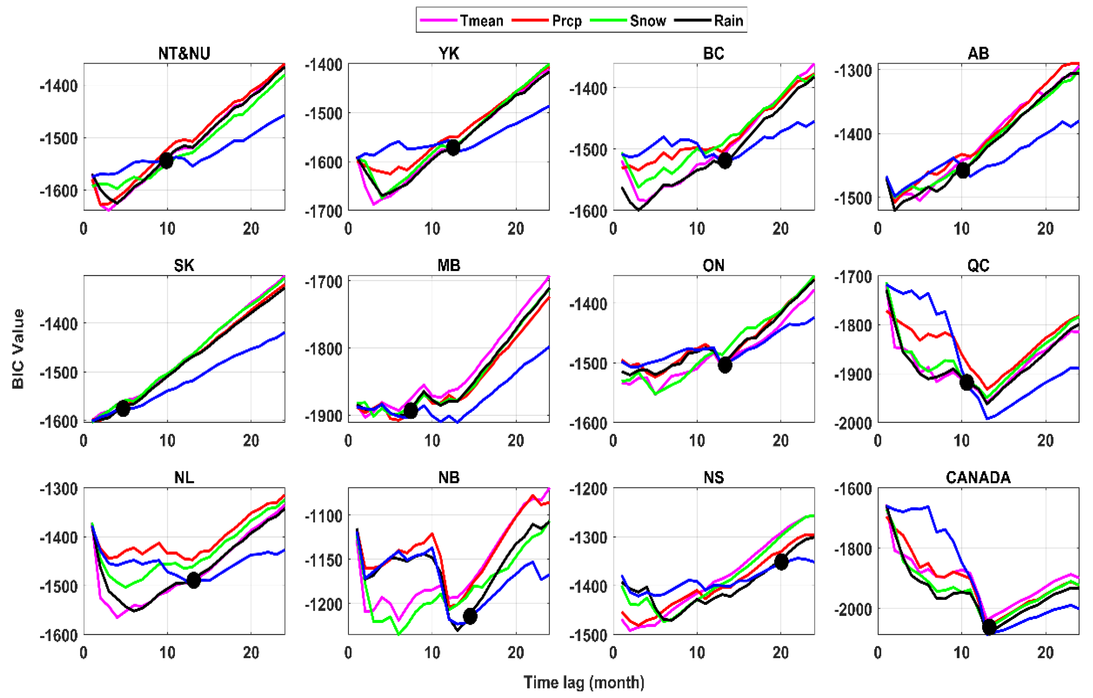
Using ARX models, monthly hydropower generation is simulated using both hydropower and one climate variable. This can provide a systematic framework to trace climatic causes of hydropower generation within each region and to reveal after how many months, considering climate variables do not contribute into a better prediction. The results of this analysis are summarized in Figure A10 in Appendix. The effective lag time is quite short in the case of SK, MB, due to the low impact of regional climate variables on forming the provincial runoff. In majority of considered regions, i.e., NU and NT, YK, BC, AB, ON, QC, NL and Canada as a whole the effect of regional climate on regional hydropower generation last up to a year. In NB and NS, the effect of climate on hydropower generation can be traced beyond a year lag time; although such effects remain mainly marginal.
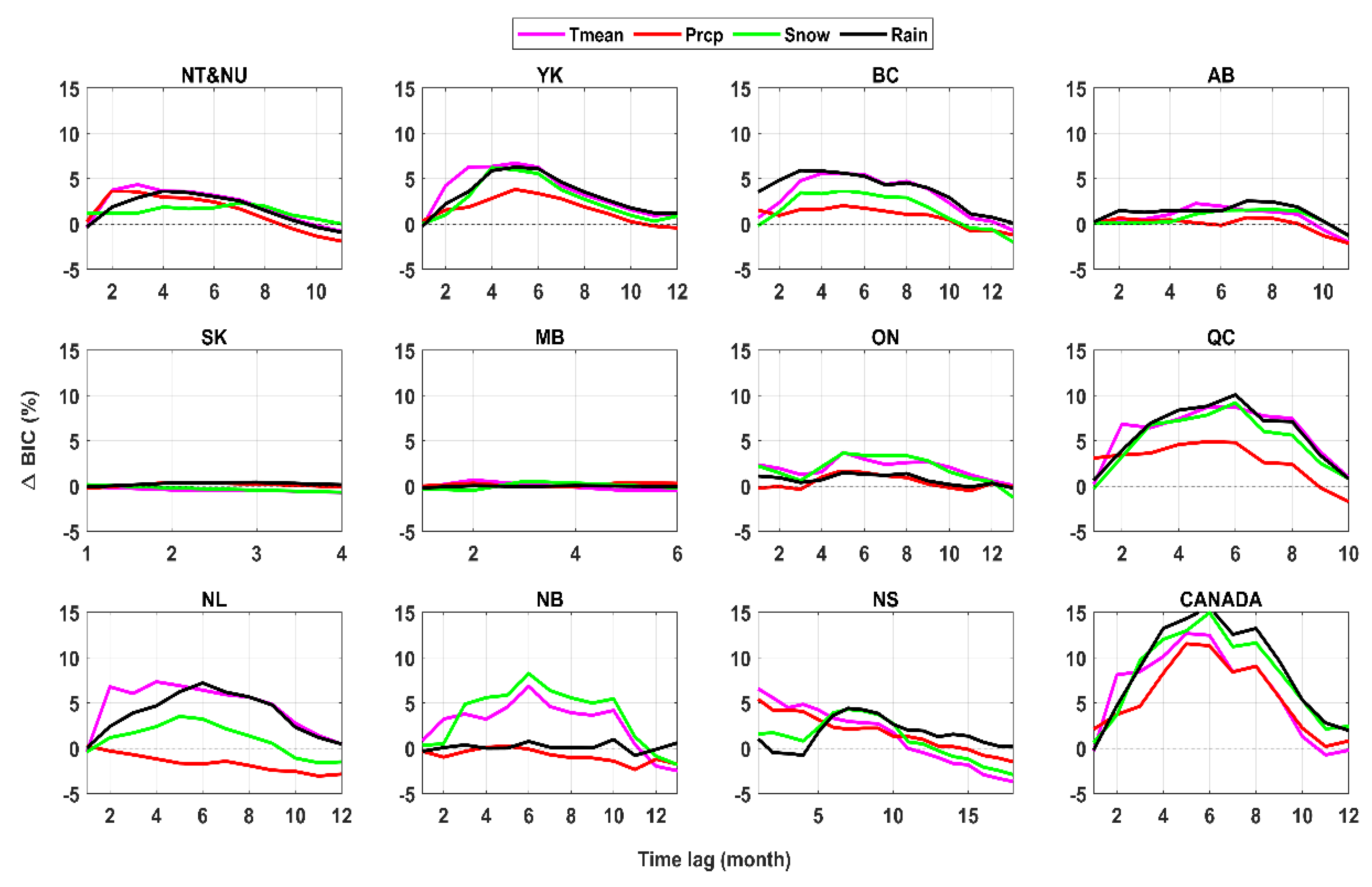
By comparing the BIC values of AR and ARX models, an objective look at the role of each climate variable in contributing into better prediction of hydropower generation across relevant time scales can be obtained. Figure 4 summarizes the findings in terms of the percentage of relative improvement in BIC, when a particular climate variable is considered for forming the ARX models. In each panel, x-axis identifies the number of lags in month and the y-axis shows the percentage of relative improvement in prediction, calculated at each time lag p as . The black dashed line indicates no improvement in the AR prediction.
For each region and time lag, the climatic variable that causes the maximum improvement in the BIC can be identified as the dominant climate variable in the considered time step. Based on the analyses made, dominant climatic causes of hydropower generation can differ based on the region and the time lag considered. In NU and NT, temperature seems to be the dominant driver in majority of time lags from one to eight months, although precipitation and rainfall mark similar improvements during earlier and later lag months, respectively. In addition, snowfall becomes the dominate driver in this region after eight months lag, which indicates the buffering effects of snow accumulation that causes delay between snowfall and hydropower generation. In YK, again temperature is the key driver of hydropower generation across a yearly timespan; however, snow and rain make almost the same improvement in prediction as temperature after four months lag. In BC, rainfall stands as the dominant climate driver, particularly within the first four months lag. After that, temperature plays almost a similar role in predictability of hydropower generation. In AB, rainfall stands as the dominant climate driver, although temperature becomes a stronger driver for five and six months lag. SK and MB show marginal effects of regional climate drivers on predicting the hydropower generation due to small contribution of regional climate in forming regional streamflow. In ON, temperature and snow stand as dominant climate causes of hydropower production, pointing on how snow accumulation and melt drive hydropower generation in this province. Similar process can be witnessed in NB. In QC, the hydropower is driven by a complex interplay between rain, snow and temperature within a 10-month time span. In NL, hydropower generation is mainly driven by temperature, although rain plays an almost similar role after six months lag. NS displays rather a complex hydropower generation process in which temperature and total precipitation are the main causes of hydropower production up to five months lag and then rainfall and snowfall takeover up to 10 months lag but only rainfall can be considered as a cause beyond 10 months and up to 15 months lag. In Canada as a whole, the total precipitation is the immediate cause of hydropower generation, which is substituted by temperature for two and three months lag. After month four and up to one year lag, rainfall and snow become dominant drivers of hydropower production, although rainfall has a more important role in predictability of hydropower generation compared to snowfall.
5.5. Predictive Models of Monthly Hydropower Production
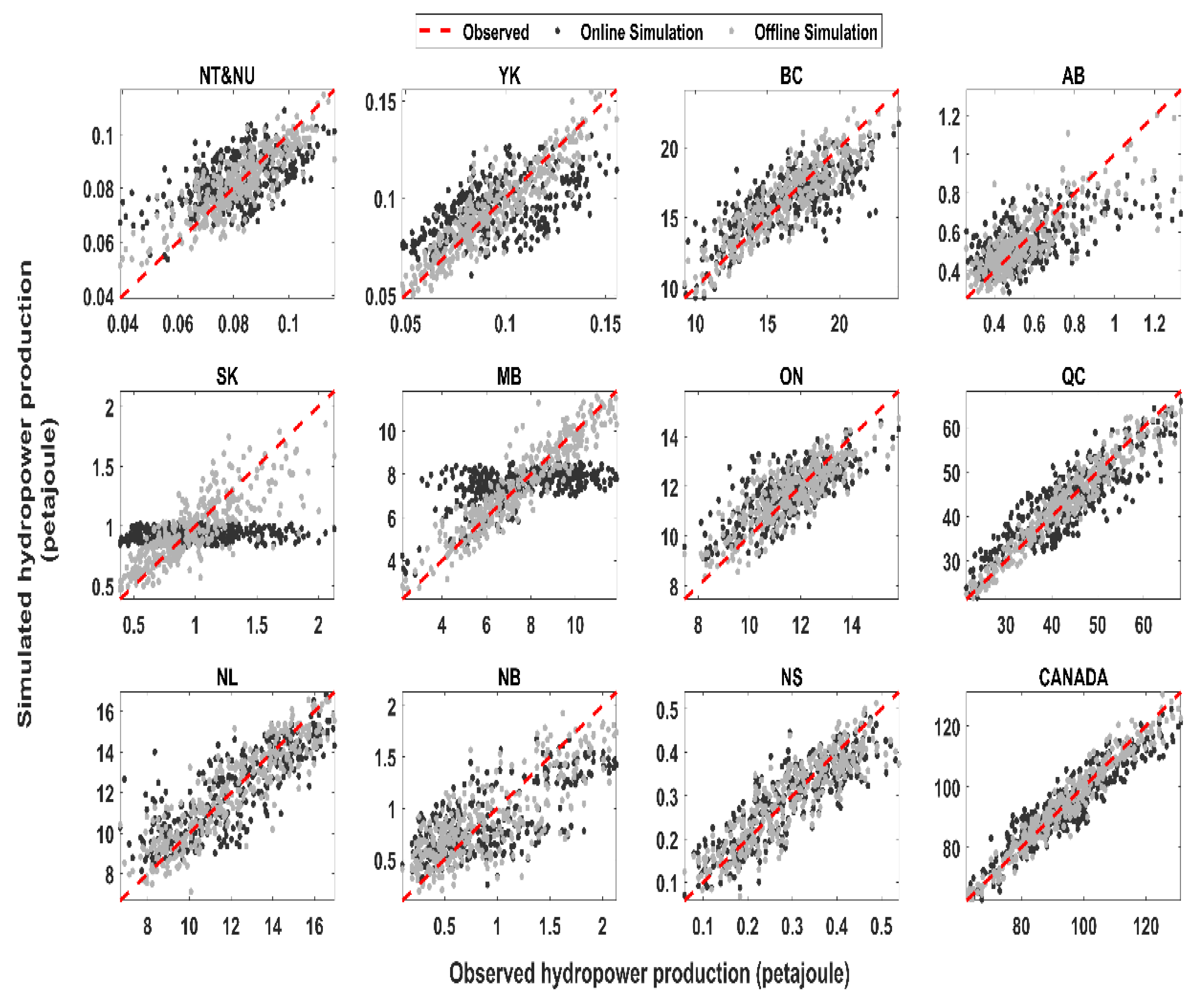
By knowing the autocorrelation structure as well as climate drivers of monthly hydropower production, it would be possible to form different predictive models for simulating hydropower generation based on the four schemes presented in Section 4.5. Accordingly, using each scheme and for each region, several competing hypotheses for modeling hydropower generation are formed by considering all possible time lags from one month to the critical number of time lag, after which there is no trace of climatic causes in the hydropower time series—see Figure A10 in Appendix. The results of standardized equation for hydropower generation can be further scaled back to the actual domain using the inverse transformation, considering minimum and maximum monthly hydropower production during the training period. The performance of developed models are inspected using three performance measures. For each region, the modeling alternative that presents the best online performance based on R2 in the testing period was chosen as the non-falsified predictive model, which can be further used for impact assessment. More details on the performance of the non-falsified predictive models are provided in Table A1 in Appendix. Figure 5 shows the observed versus online and offline simulations of hydropower production across Canadian regions. As it is obvious, in offline simulation modes, the non-falsified models are able to track the monthly time series of hydropower production very well. Having said that, by moving to online simulation, the performance of the predictive models declines substantially particularly in SK and MB, where regional climate variables have marginal effect in the formation of hydropower production. Some discrepancies are also seen in NB, ON and YK; however, the predictive models can describe more than 75% of the variance within the observed data in Canada as a whole. This can provide an opportunity to use these predictive models for impact assessment.
6. Expected Change in Hydropower Production Potential under Historical Climate Trends
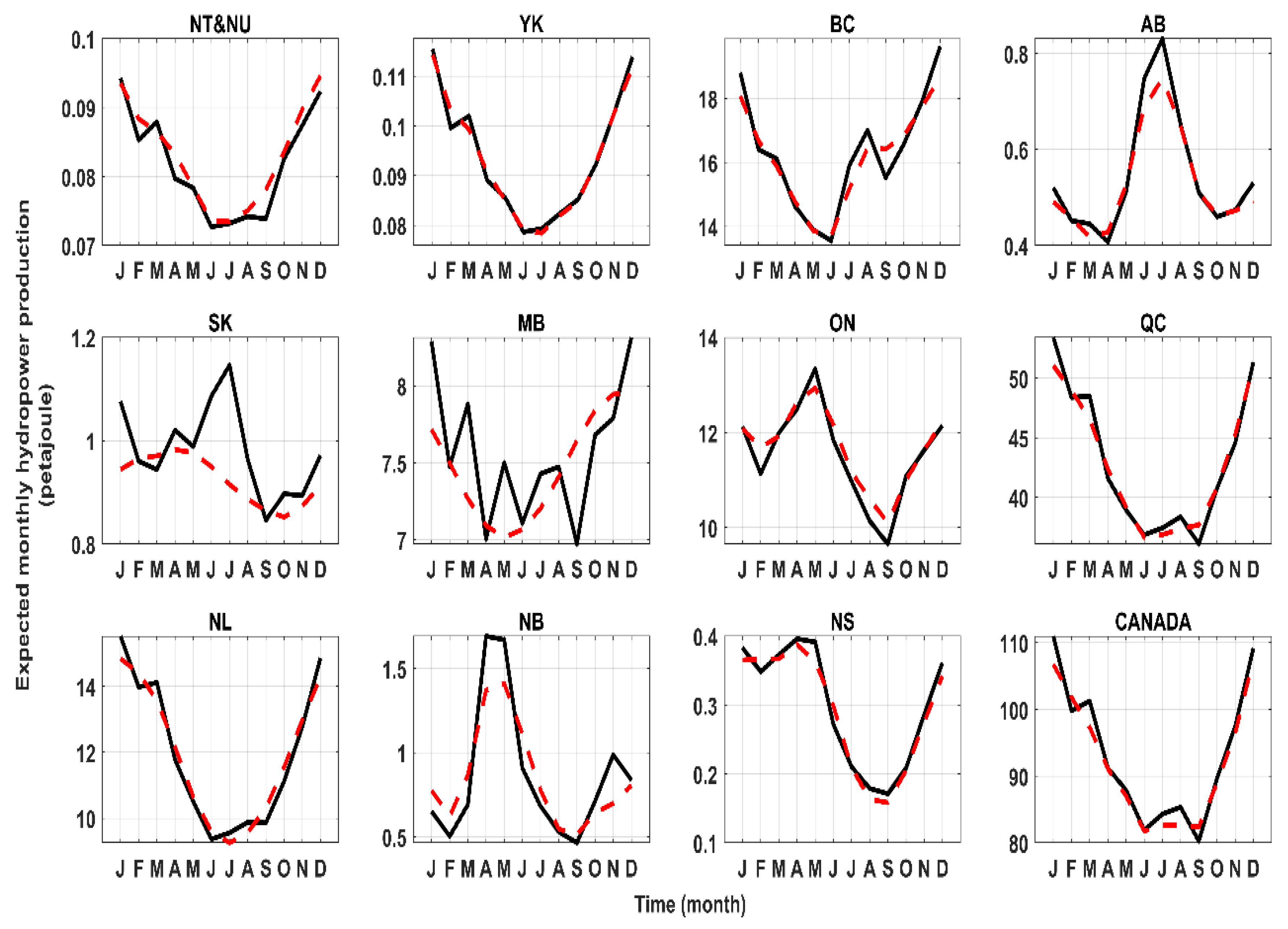
Before implementing the non-falsified models for impact assessment, the reliability of predictive models should be inspected in terms of their performance in tracking the expected monthly hydropower production during the historical period. To do so, we introduce the historical climate data to non-falsified models to simulate the monthly hydropower time series in the online mode. We then average all the yearly hydropower profiles to come up with an expected time series of monthly hydropower production in a typical year. The results are shown in Figure 6, revealing that the expected values of hydropower production gathered from simulations are close to the observed values in most of the Canadian regions, except in SK and MB.
We categorize the confidence level of the non-falsified models in simulating the expected monthly hydropower production based on the correlation coefficient, , as well as percentage of relative error between observed and simulated monthly hydropower production—see Table 2. In general, the confidence in the non-falsified models for capturing the expected monthly hydropower production is “good” and “very good” in ten out of twelve jurisdictions considered and therefore it is legitimate to use their corresponding predictive models for impact assessment. We therefore do not include SK and MB in our assessment, as the predictive models are not credible.
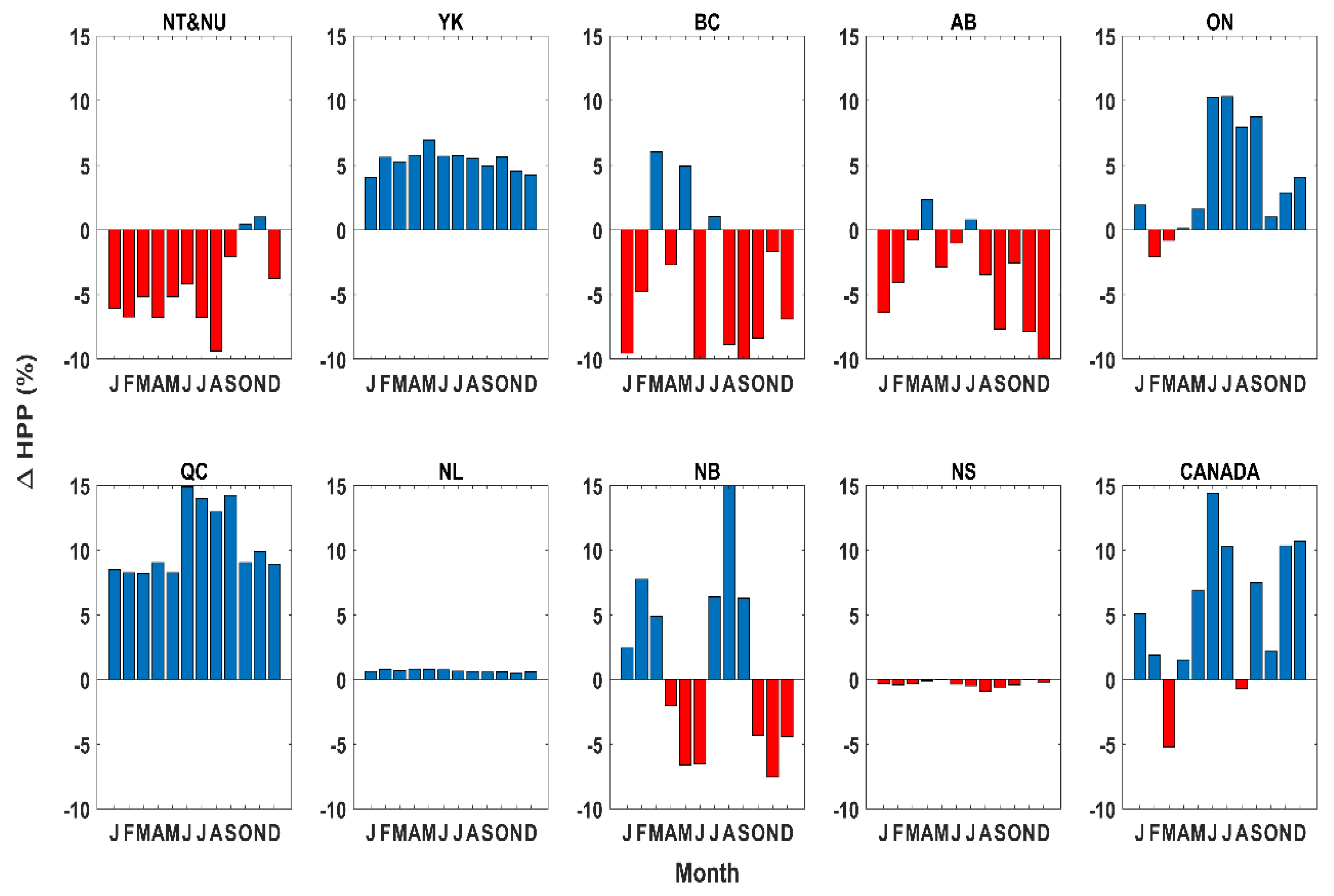
To investigate the impact of existing trends on hydropower production, changes in monthly climate variables in the course of 31 years (i.e., monthly trend values multiplied by 31) are added as delta factors to the observed monthly climate variables. This implies that no shift in timing and duration of seasonal and/or interannual variability is considered. The synthetic data are then fed into the non-falsified predictive models. Accordingly, the difference between expected monthly generation, simulated under observed and perturbed climate data, can reveal the expected gain/loss of hydropower production in light of the existing trends in climate variables. The results of this analysis are shown in Figure 7.
In NU and NT, there are lower expected values in all months except October and November. The maximum expected decrement in hydropower production potential takes place around 10% in August. On the other hand, hydropower is expected to increase under the continuation of historical trends in climate variables across YK, where the maximum gain will occur in March by 8% and other months will experience increases in generation by around 5%. In BC, the expected effect of continuation in hydropower production potential varies throughout a typical year, but it decreases during summer and fall. The maximum gain will be in March around 8%, while hydropower can decrease by around 10% in September. In AB, the hydropower production potential experience a maximum increase of 3% in April but can also suffer from maximum expected loss of 10%, captured in December. In ON, hydropower production potential is expected to increase in spring, summer, and fall but can decrease marginally in winter. The maximum gain in hydropower production potential will occur in June and July by around 10%. Higher hydropower production potential is expected under the continuation of climate trends in QC, with the maximum gain of around 15%, taking place in June. NL and NS will experience marginal changes in their production potential. In NB, hydropower production potential is expected to increase during the winter and summer but to decrease in spring and fall. The maximum gain in this region is expected to take place in August by around 15%. Looking at Canada as a whole, hydropower production potential is expected to increase in all months except in March and August. The maximum gain is expected by around 15% in June and the maximum loss is in March by around 5%.
7. Summary, Conclusions and Further Remarks
Due to imposing significant changes in characteristics of water availability in time and space, climate change can be a critical stressor to hydropower production, locally, regionally, and globally. This has a particular importance in a country like Canada, in which hydropower production has an important role in both domestic and international electricity supply. Despite this importance, current studies are limited due to two key reasons. First, the majority of current impact assessments performed at small samples of power plants and/or river basins and therefore they do not provide a large-scale understanding, particularly across political jurisdictions where management decisions are made. In addition, current studies mainly adopt a top-down impact assessment based on using climate, hydrological, and energy simulation models. These modeling technologies are still incomplete and therefore impose large uncertainties into assessment results. To avoid these limitations, here we develop a fully bottom-up and empirical-based approach to assess the impact of changing climate across Canadian political regions. On the one hand, we use historical trends in regional climate variables as a plausible scenario to quantify the changing climate. On the other hand, the knowledge of dependency and causal links between climate variables and hydropower production across political jurisdictions is used as a basis to develop a set of predictive data-driven models, with which the expected gain/loss in hydropower production potential can be estimated under the quantification of historical climatic trends.
Our results of monthly, seasonal, and annual climate trend analyses across political regions in Canada confirm previous findings that Canada is getting warmer and wetter with more contribution from rainfall than snow. Warming temperature, however, stands as dominant signal of historical climate change across Canadian regions, as the rates of warming across temporal and spatial scales are more significant, compared to the incline in rainfall amount and/or decline in snowfall. In addition, our analyses reveal the regional autocorrelation structure in hydropower production and dependencies between climate variables and hydropower production across Canadian regions. In terms of autocorrelation structure, our analyses show three distinct forms of autocorrelation in monthly regional hydropower production, related to short-, mid- and long-range memory in monthly time series of hydropower production. We highlight strong dependencies between climate variables and hydropower production, which can be highly variant in time and space.
Having said that, we note that the statistical dependency does not necessarily mean causal links between climate variables and hydropower production; and therefore, we use a formal casualty test to trace the climatic causes of hydropower production across time and space. Despite regional differences in climatic causes of hydropower production, we show that considering climatic variables up to one-year lag can improve the predictability of hydropower production. There is however an exception in Saskatchewan and Manitoba, where the water availability is mainly contributed from upstream province of Alberta. Accordingly, we establish a wide range of modeling alternatives to predict monthly hydropower production, based on previous values of hydropower production and climatic causes at each Canadian region. We make a rigorous intercomparison among modeling hypotheses based on a number of goodness-of-fit measures and in two online and offline simulation modes. For each region, we then select the modeling option that resembles the highest coefficient of determination during testing period and in online simulation mode. We show that these non-falsified predictive models are able to track the expected monthly hydropower production very well across Canadian regions, except in Saskatchewan and Manitoba. By knowing the climatic trends and a non-falsified predictive model at each region, we can assess how the hydropower production potential can change under continuation of climatic trends. For this purpose, we perturb the historical time series of climate by adding the corresponding climatic shift in the course of 31 years using the identified trends, and accordingly, feed the synthesized time series to the predictive model to calculate the expected change in the hydropower production potential. Our assessment show that Canada as a whole can benefit from higher monthly hydropower production potential under continuation of climatic trends. This conclusion however is subject to large variability across political regions, as for instance the production potential can significantly decrease in BC, NU and NT as well as AB.
It should be noted that our findings are only one possible narrative that portrays Canadian hydropower production under uncertain climate futures. As it was pointed earlier, hydropower production is also dependent on electricity demand as well as production capacity, for which we did not consider any change under future condition. As a result, our findings should be taken as an assessment of change in hydropower production potential under one possible scenario for future climate. We would like to emphasize on the inherent uncertainty in this climate scenario, as there is no guarantee that historical climate trends remain unchanged in the future. Yet, we believe that this scenario can provide a tangible baseline narrative to inform both public and decision makers on the impact of climate change on Canadian hydropower production. In addition, it should be noted that we consider each political region as a lumped production unit in which fluctuation around expected production can be described by variations in regional climate variables. Although, our modeling results show that this can be a legitimate assumption except in Saskatchewan and Manitoba, our findings are only relevant at the spatial and temporal scales in which causal links between climate variables and hydropower productions are considered, i.e., monthly production across political jurisdictions. We therefore do not suggest extrapolating these results into other spatial and temporal scales. Last but not the least, other data-driven methodologies can be used to describe the linkage between climate variables and hydropower production at the regional scale [120,121]; and therefore, there is an uncertainty in our assessment due to the uncertainty in non-falsified predictive models. We recognize that every single assessment of future conditions is inherently subject to deep uncertainty and our study is no exception. Having said that, our findings provide a fresh look at the possible gain/loss in hydropower production potential across Canadian political regions. We hope our study can trigger more efforts towards understanding challenges and opportunities in Canada’s hydropower production under climatic changes.
Author Contributions
Conceptualization and design, A.N. and A.A.J.; Data gathering, A.A.J.; Methodology, A.N. and A.A.J.; Data analysis, A.A.J.; Coding and model development, A.A.J.; Interpretation of results, A.A.J. and A.N.; Design of narrative and visualization, A.N. and A.A.J.; Preparation of figures, A.A.J.; Writing of first draft, A.A.J.; Editing and revising the initial draft, A.N. and A.A.J.; Project administration, A.N.; Funding acquisition, A.N.
Funding
This research was funded by Concordia University’s Strategic Hire funding scheme as well as NSERC Discovery Grant (Grant number: RGPIN/5470-2016), extended to the corresponding author.
Acknowledgments
Authors would like to thank the editor and two anonymous reviewers for their constructive comments, which improved the quality of this piece as a whole.
Conflicts of Interest
The authors declare no conflict of interest.
Appendix A
Figure A1.
Monthly hydropower productions in Canada across provincial, territorial, and country-wide scales.
Figure A1.
Monthly hydropower productions in Canada across provincial, territorial, and country-wide scales.

Figure A2.
Distribution of climate stations providing the data support for precipitation, rainfall, and snowfall amounts in this study.
Figure A2.
Distribution of climate stations providing the data support for precipitation, rainfall, and snowfall amounts in this study.

Figure A3.
Distribution of climate stations providing the data support for temperature amounts in this study.
Figure A3.
Distribution of climate stations providing the data support for temperature amounts in this study.

Figure A4.
Anomaly in annual mean temperature across climate stations clustered at each political region (grey envelope) versus anomaly in the corresponding upscaled regional temperature (red line).
Figure A4.
Anomaly in annual mean temperature across climate stations clustered at each political region (grey envelope) versus anomaly in the corresponding upscaled regional temperature (red line).

Figure A5.
Anomaly in annual mean precipitation across climate stations clustered at each political region (grey envelope) versus anomaly in the corresponding upscaled regional precipitation (red line).
Figure A5.
Anomaly in annual mean precipitation across climate stations clustered at each political region (grey envelope) versus anomaly in the corresponding upscaled regional precipitation (red line).

Figure A6.
Anomaly in annual mean snowfall across climate stations clustered at each political region (grey envelope) versus anomaly in the corresponding upscaled regional snowfall (red line).
Figure A6.
Anomaly in annual mean snowfall across climate stations clustered at each political region (grey envelope) versus anomaly in the corresponding upscaled regional snowfall (red line).

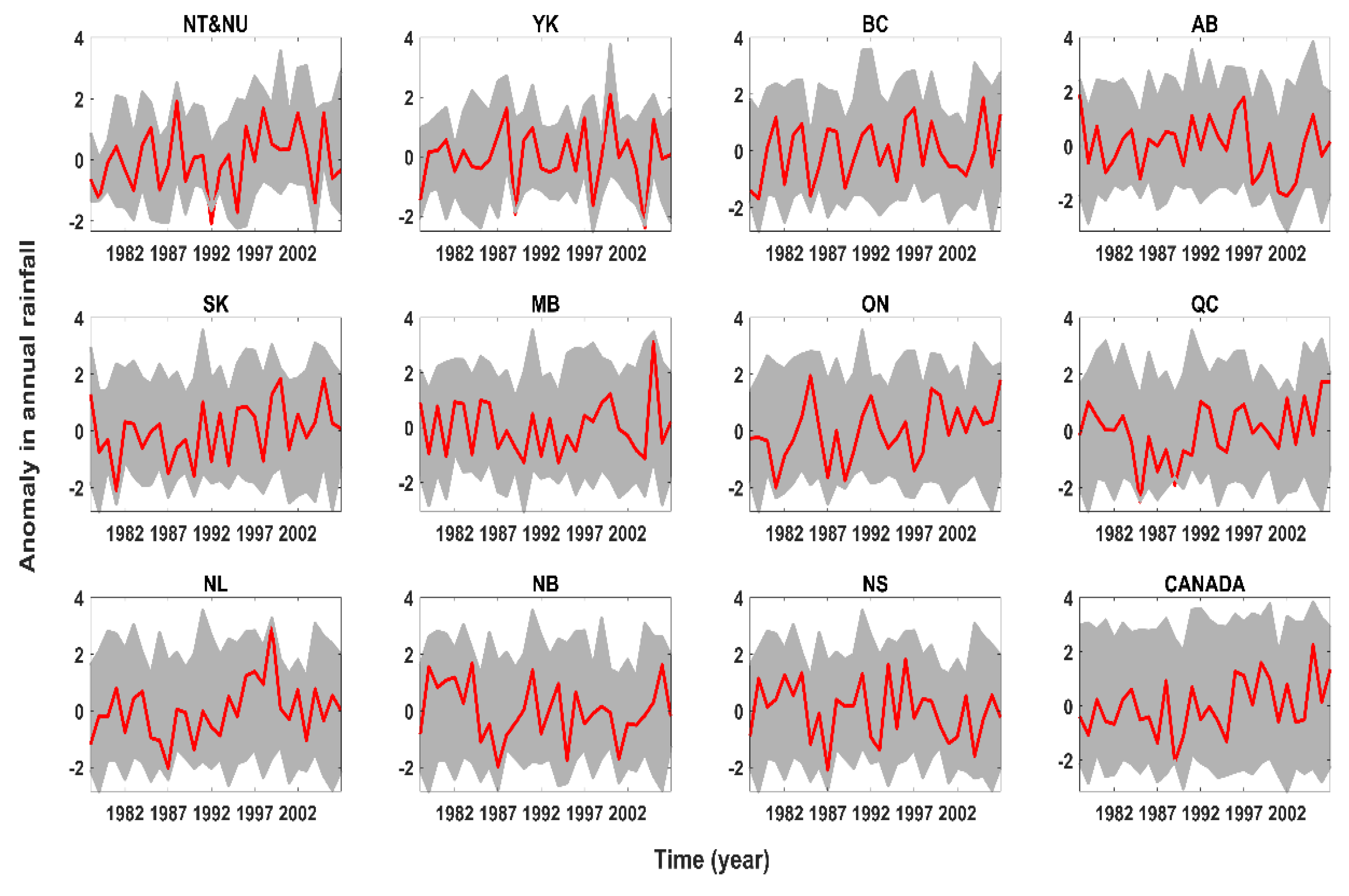
Figure A7.
Anomaly in annual mean rainfall across climate stations clustered at each political region (grey envelope) versus anomaly in the corresponding upscaled regional rainfall (red line).
Figure A7.
Anomaly in annual mean rainfall across climate stations clustered at each political region (grey envelope) versus anomaly in the corresponding upscaled regional rainfall (red line).

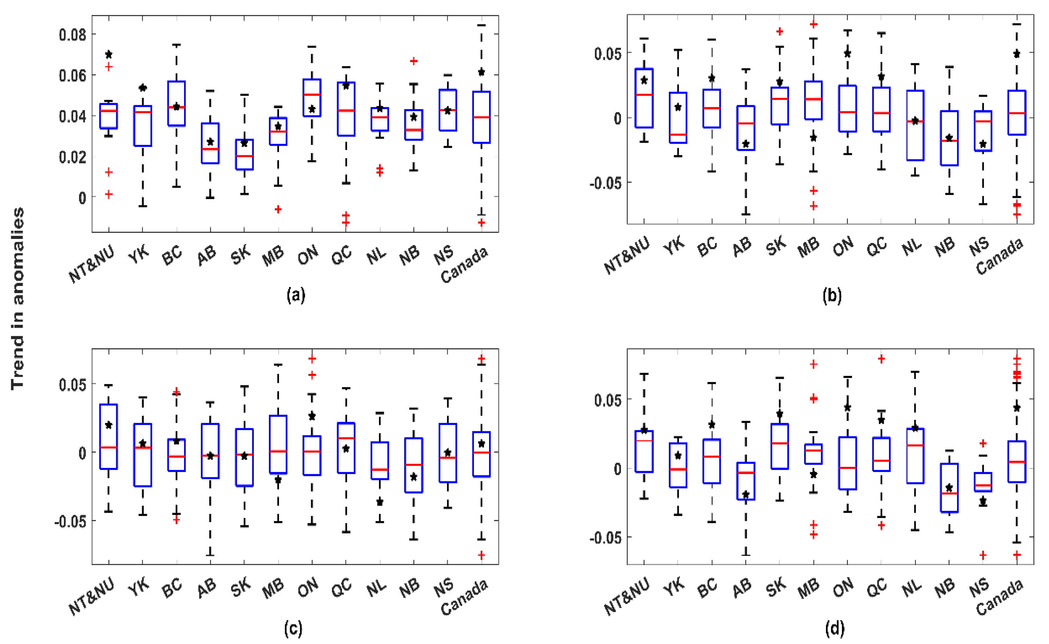
Figure A8.
The trends in the anomalies of (a) mean annual temperature, (b) total precipitation, (c) total snowfall, and (d) total rainfall across climate stations at each political region (boxplots) versus the trend in the anomaly of corresponding upscaled regional climate variable (black dots).
Figure A8.
The trends in the anomalies of (a) mean annual temperature, (b) total precipitation, (c) total snowfall, and (d) total rainfall across climate stations at each political region (boxplots) versus the trend in the anomaly of corresponding upscaled regional climate variable (black dots).

Figure A9.
Autocorrelation structure in monthly hydropower production across Canadian regions; red lines are identifying the 95% significance threshold for autocorrelation estimates.
Figure A9.
Autocorrelation structure in monthly hydropower production across Canadian regions; red lines are identifying the 95% significance threshold for autocorrelation estimates.

Figure A10.
BIC values for AR and Auto Regressive with Exogenous variable (ARX) models of monthly hydropower production. In ARX models each climate variable is considered separately. Black solid dots identify time lag beyond which the impact of climate variables cannot be traced.
Figure A10.
BIC values for AR and Auto Regressive with Exogenous variable (ARX) models of monthly hydropower production. In ARX models each climate variable is considered separately. Black solid dots identify time lag beyond which the impact of climate variables cannot be traced.


Table A1.
Setup and performance of non-falsified predictive models for hydropower generation across Canadian Regions.
Table A1.
Setup and performance of non-falsified predictive models for hydropower generation across Canadian Regions.
| Region | Scheme | # of Lags | BIC (Online) | BIC (Offline) | R2 (Online) | R2 (Offline) | RMSE (Online) | RMSE (Offline) |
|---|---|---|---|---|---|---|---|---|
| NT&NU | D | 11 | 6126.72 | 5787.89 | 0.28 | 0.71 | 0.0006 | 0.0004 |
| YK | D | 12 | 6520.39 | 6004.94 | 0.32 | 0.84 | 0.0010 | 0.0005 |
| BC | D | 12 | 9816.36 | 9564.69 | 0.61 | 0.81 | 0.1009 | 0.0711 |
| AB | D | 8 | 7978.56 | 7778.86 | 0.40 | 0.65 | 0.0079 | 0.0060 |
| SK | A | 1 | 8515.76 | 8105.06 | 0.02 | 0.67 | 0.0177 | 0.0102 |
| MB | A | 2 | 9717.99 | 9057.81 | 0.30 | 0.88 | 0.0915 | 0.0375 |
| ON | D | 12 | 9329.26 | 9191.53 | 0.54 | 0.69 | 0.0517 | 0.0427 |
| QC | D | 10 | 10,496.78 | 10,052.97 | 0.79 | 0.94 | 0.2555 | 0.1384 |
| NL | B | 7 | 9507.62 | 9333.78 | 0.71 | 0.82 | 0.0727 | 0.0573 |
| NB | B | 12 | 8419.53 | 8333.38 | 0.52 | 0.61 | 0.0185 | 0.0164 |
| NS | B | 12 | 7153.24 | 7100.78 | 0.75 | 0.78 | 0.0028 | 0.0026 |
| CANADA | D | 12 | 10,595.57 | 10,241.35 | 0.87 | 0.95 | 0.2954 | 0.1806 |
References
- International Renewable Energy Agency (IRENA). Renewable Energy Benefits: Understandinf the Socio-Economics; International Renewable Energy Agency (IRENA): Abu Dhabi, United Arab Emirates, 2017. [Google Scholar]
- International Energy Agency (IEA). World Energy Outlook 2011; International Energy Agency (IEA): Paris, France, 2011. [Google Scholar]
- UNFCCC. Paris Agreement; UNFCCC: Bonn, Germany, 2015. [Google Scholar]
- BP Energy, P.L.C. BP Statistical Review of World Energy; BP Energy P.L.C.: London, UK, 2019. [Google Scholar]
- Energy Information Administration (EIA). International Energy Outlook 2010; Energy Information Administration (EIA): Washington, DC, USA, 2010.
- Energy Information Administration (EIA). Canada Is One of the World's Five Largest Energy Producers and Is the Principal Source of U.S. Energy Imports; Energy Information Administration (EIA): Washington, DC, USA, 2011.
- Hydro-Quebec. Annual Report 2010; Hydro-Quebec: Montreal, QC, Canada, 2011. [Google Scholar]
- Natalia Lis, C.C.; Ektvedt, I. Michael Nadew, Ken Newel, Sara Tsang, and Cassandra Wilde. In Canada’s Renewable Power Landscape Energy Market Analysis; National Energy Board: Calgary, AB, Canada, 2016. [Google Scholar]
- Canada—A Global Leader in Renewable Energy Enhancing Collaboration on Renewable Energy Technologies. In Proceedings of the Energy and Mines Ministers’ Conference, Yellowknife, NT, Canada, 26–27 August 2013.
- Canadian Hydropower Association. Report of Activities 2014–2015; Canadian Hydropower Association: Ottawa, ON, Canada, 2015.
- Contreras-Lisperguer, R.; de Cuba, K. The Potential Impact of Climate Change on the Energy Sector in the Caribbean Region; The Organization of American States: Washington, DC, USA, 2008. [Google Scholar]
- Robinson, P.J. Climate change and hydropower generation. In. J. Climatol. J. R. Meteorol. Soc. 1997, 17, 983–996. [Google Scholar] [CrossRef]
- Wagner, T.; Themeßl, M.; Schüppel, A.; Gobiet, A.; Stigler, H.; Birk, S. Impacts of climate change on stream flow and hydro power generation in the Alpine region. Environ. Earth Sci. 2017, 76, 4. [Google Scholar] [CrossRef]
- Adam, J.C.; Lettenmaier, D.P. Application of new precipitation and reconstructed streamflow products to streamflow trend attribution in northern Eurasia. J. Clim. 2008, 21, 1807–1828. [Google Scholar] [CrossRef]
- Bonfils, C.; Santer, B.D.; Pierce, D.W.; Hidalgo, H.G.; Bala, G.; Das, T.; Barnett, T.P.; Cayan, D.R.; Doutriaux, C.; Wood, A.W. Detection and attribution of temperature changes in the mountainous western United States. J. Clim. 2008, 21, 6404–6424. [Google Scholar] [CrossRef]
- Harrison, G.P.; Wallace, A.R. Climate change impacts on renewable energy–is it all hot air? In Proceedings of the World Renewable Energy Congress (WREC2005), Aberdeen, UK, 22–27 May 2005. [Google Scholar]
- IPCC-WG, I. Climate Change 2000, Third Assessment Report; Cambridge University Press: Cambridge, UK, 2001. [Google Scholar]
- Nicholls, N.; Gruza, G.; Jouzel, J.; Karl, T.; Ogallo, L.; Parker, D. Observed Climate Variability and Change; University Press Cambridge: Cambridge, UK, 1996. [Google Scholar]
- Schär, C.; Vidale, P.L.; Lüthi, D.; Frei, C.; Häberli, C.; Liniger, M.A.; Appenzeller, C. The role of increasing temperature variability in European summer heatwaves. Nature 2017, 427, 332. [Google Scholar] [CrossRef] [PubMed]
- Vincent, L.; Zhang, X.; Brown, R.; Feng, Y.; Mekis, E.; Milewska, E.; Wan, H.; Wang, X. Observed trends in Canada’s climate and influence of low-frequency variability modes. J. Clim. 2015, 28, 4545–4560. [Google Scholar] [CrossRef]
- Whitfield, P.H.; Cannon, A.J. Recent variations in climate and hydrology in Canada. Can. Water Res. J. 2000, 25, 19–65. [Google Scholar] [CrossRef]
- Yagouti, A.; Boulet, G.; Vescovi, L. Homogénéisation des séries de température et analyse de la variabilité spatio-temporelle de ces séries au Québec méridional; Ouranos: Montreal, QC, Canada, 2006; p. 154. [Google Scholar]
- Zhang, X.; Vincent, L.A.; Hogg, W.; Niitsoo, A. Temperature and precipitation trends in Canada during the 20th century. Atmosph. Ocean 2000, 38, 395–429. [Google Scholar] [CrossRef]
- Bush, E.; Gillett, N.; Watson, E.; Fyfe, J.; Vogel, F.; Swart, N. Understanding Observed Global Climate Change. In Canada’s Changing Climate Report; Bush, E., Lemmen, D.S., Eds.; Government of Canada: Ottawa, ON, Canada, 2019; pp. 24–72. [Google Scholar]
- IPCC. Climate Change 2014: Impacts, Adaptation, and Vulnerability. Part A:Global and Sectoral Aspects; Contribution of Working Group II to the FifthAssessment Report of the Intergovernmental Panel on Climate Change; Field, C.B., Barros, V.R., Dokken, D.J., Mach, K.L., Mastrandrea, M.D., Chatterjee, M., Ebi, K.L., Estrada, Y.O., Genova, R.C., et al., Eds.; Cambridge University Press: Cambridge, UK; New York, NY, USA, 2014; p. 1132. [Google Scholar]
- Dai, A.; Trenberth, K.E.; Karl, T.R. Global variations in droughts and wet spells: 1900–1995. Geophys. Res. Lett. 1998, 25, 3367–3370. [Google Scholar] [CrossRef]
- Trenberth, K.E.; Dai, A.; Rasmussen, R.M.; Parsons, D.B. The changing character of precipitation. Bull. Am. Meteorol. Soc. 2003, 84, 1205–1218. [Google Scholar] [CrossRef]
- Hartmann, D.L.; Tank, A.M.K.; Rusticucci, M.; Alexander, L.V.; Brönnimann, S.; Charabi, Y.A.R.; Dentener, F.J.; Dlugokencky, E.J.; Easterling, D.R.; Kaplan, A. Observations: Atmosphere and surface. In Climate Change 2013 the Physical Science Basis: Working Group I Contribution to the Fifth Assessment Report of the Intergovernmental Panel on Climate Change; Cambridge University Press: Cambridge, UK, 2013. [Google Scholar]
- Iimi, A. Estimating Global Climate Change Impacts on Hydropower Projects: Applications in India, Sri Lanka and Vietnam; The World Bank: Washington, DC, USA, 2007. [Google Scholar]
- Dore, M.H. Climate change and changes in global precipitation patterns: What do we know? Environ. Int. 2005, 31, 1167–1181. [Google Scholar] [CrossRef] [PubMed]
- Hulme, M.; Osborn, T.J.; Johns, T.C. Precipitation sensitivity to global warming: Comparison of observations with HadCM2 simulations. Geophys. Res. Lett. 1998, 25, 3379–3382. [Google Scholar] [CrossRef]
- Jones, P.; Hulme, M. Calculating regional climatic time series for temperature and precipitation: Methods and illustrations. Int. J. Climatol. J. R. Meteorol. Soc. 1996, 16, 361–377. [Google Scholar] [CrossRef]
- Déry, S.J.; Wood, E. Decreasing river discharge in northern Canada. Geophys. Res. Lett. 2005, 32. [Google Scholar] [CrossRef] [Green Version]
- Meehl, G.A.; Stocker, T.F.; Collins, W.D.; Friedlingstein, P.; Gaye, T.; Gregory, J.M.; Kitoh, A.; Knutti, R.; Murphy, J.M.; Noda, A. Global Climate Projections; Cambridge University Press: Cambridge, UK, 2007. [Google Scholar]
- Stone, D.A.; Weaver, A.J.; Zwiers, F.W. Trends in Canadian precipitation intensity. Atmosph. Ocean. 2000, 38, 321–347. [Google Scholar] [CrossRef]
- Allard, M.; Calmels, F.; Fortier, D.; Laurent, C.; L’Hérault, E.; Vinet, F. Cartographie des conditions de pergélisol dans les communautés du Nunavik en vue de l’adaptation au réchauffement climatique. In Rapport au Fonds D’action Pour le Changement Climatique et à Ouranos; Ouranos: Montreal, QC, Canada, 2007. [Google Scholar]
- Barnett, T.P.; Adam, J.C.; Lettenmaier, D.P. Potential impacts of a warming climate on water availability in snow-dominated regions. Nature 2005, 438, 303–309. [Google Scholar] [CrossRef] [PubMed]
- Chun, K.P.; Wheater, H.S.; Nazemi, A.; Khaliq, M.N. Precipitation downscaling in Canadian Prairie Provinces using the LARS-WG and GLM approaches. Can. Water Res. J. 2013, 38, 311–332. [Google Scholar] [CrossRef]
- Bates, B.; Kundzewicz, Z.; Wu, S.; Palutikof, J.P. Climate Change and Water; Intergovernmental Panel on Climate Change, IPCC Secretariat: Geneva, Switzerland, 2008. [Google Scholar]
- IPCC. Climate Change 2007: The Physical Science Basis; Contribution of Working Group I to the Fourth Assessment Report of the Intergovernmental Panel on Climate Change; Solomon, S., Qin, D., Manning, M., Chen, Z., Marquis, M., Averyt, K.B., Tignor, M., Miller, H., Eds.; Cambridge University Press: Cambridge, UK; New York, NY, USA, 2007; p. 996. [Google Scholar]
- Emori, S.; Brown, S. Dynamic and thermodynamic changes in mean and extreme precipitation under changed climate. Geophys. Res. Lett. 2005, 32. [Google Scholar] [CrossRef]
- Kharin, V.V.; Zwiers, F.W. Climate predictions with multimodel ensembles. J. Clim. 2002, 15, 793–799. [Google Scholar] [CrossRef]
- Kumar, A.; Schei, T.; Ahenkorah, A.; Caceres Rodriguez, R.; Devernay, J.; Freitas, M.; Hall, D.; Killingtveit, Å.; Liu, Z. Hydropower. In ‘IPCC Special Report on Renewable Energy Sources and Climate Change Mitigation’; The Intergovernmental Panel on Climate Change: Geneva, Switzerland, 2011. [Google Scholar]
- Shu, J.; Qu, J.; Motha, R.; Xu, J.; Dong, D. Impacts of climate change on hydropower development and sustainability: A review. IOP Conf. Ser. Earth Environ. Sci. 2018, 163, 012126. [Google Scholar] [CrossRef]
- Hamududu, B.; Killingtveit, A. Assessing climate change impacts on global hydropower. Energies 2012, 5, 305–322. [Google Scholar] [CrossRef]
- Killingtveit, Å.; Adera, A.G. Climate Change and Impact on Water Resources and Hydropower-The Case of Vanatori Neamt in the Carpathian Region of Romania; NTNU: Trondheim, Norway, 2017. [Google Scholar]
- Teotónio, C.; Fortes, P.; Roebeling, P.; Rodriguez, M.; Robaina-Alves, M. Assessing the impacts of climate change on hydropower generation and the power sector in Portugal: A partial equilibrium approach. Renew. Sustain. Energy Rev. 2017, 74, 788–799. [Google Scholar] [CrossRef]
- Turner, S.W.; Ng, J.Y.; Galelli, S. Examining global electricity supply vulnerability to climate change using a high-fidelity hydropower dam model. Sci. Total Environ. 2017, 590, 663–675. [Google Scholar] [CrossRef] [PubMed]
- Uamusse, M.M.; Aljaradin, M.; Nilsson, E.; Persson, K.M. Climate Change observations into Hydropower in Mozambique. Energy Proc. 2017, 138, 592–597. [Google Scholar] [CrossRef]
- Cherry, J.E.; Knapp, C.; Trainor, S.; Ray, A.J.; Tedesche, M.; Walker, S. Planning for climate change impacts on hydropower in the Far North. Hydrol. Earth Syst. Sci. 2017, 21, 133–151. [Google Scholar] [CrossRef] [Green Version]
- Minville, M.; Krau, S.; Brissette, F.; Leconte, R. Behaviour and performance of a water resource system in Québec (Canada) under adapted operating policies in a climate change context. Water Res. Manag. 2010, 24, 1333–1352. [Google Scholar] [CrossRef]
- Shevnina, E.; Pilli-Sihvola, K.; Haavisto, R.; Vihma, T.; Silaev, A. Climate Change Will Increase Potential Hydropower Production in Six Arctic Council Member Countries Based on Probabilistic Hydrological Projections; Copernicus Publications: Göttingen, Germany, 2018. [Google Scholar]
- Caruso, B.; King, R.; Newton, S.; Zammit, C. Simulation of climate change effects on hydropower operations in mountain headwater lakes, New Zealand. River Res. Appl. 2017, 33, 147–161. [Google Scholar] [CrossRef]
- Chilkoti, V.; Bolisetti, T.; Balachandar, R. Climate change impact assessment on hydropower generation using multi-model climate ensemble. Renew. Energy 2017, 109, 510–517. [Google Scholar] [CrossRef]
- Ehrbar, D.; Schmocker, L.; Vetsch, D.; Boes, R. Hydropower potential in the periglacial environment of Switzerland under climate change. Sustainability 2018, 10, 2794. [Google Scholar]
- Hasan, M.M.; Wyseure, G. Impact of climate change on hydropower generation in Rio Jubones Basin, Ecuador. Water Sci. Eng. 2018, 11, 157–166. [Google Scholar] [CrossRef]
- Forrest, K.; Tarroja, B.; Chiang, F.; AghaKouchak, A.; Samuelsen, S. Assessing climate change impacts on California hydropower generation and ancillary services provision. Clim. Chang. 2018, 151, 395–412. [Google Scholar] [CrossRef]
- Khadka Mishra, S.; Hayse, J.; Veselka, T.; Yan, E.; Kayastha, R.B.; LaGory, K.; McDonald, K.; Steiner, N. An Integrated Assessment Approach for Estimating the Economic Values of Climate Change Sensitive River Systems An Application to Hydropower and Fisheries in a Himalayan River, Trishuli. Environ. Sci. Policy 2018, 87, 102–111. [Google Scholar] [CrossRef]
- Minville, M.; Brissette, F.; Leconte, R. Impacts and uncertainty of climate change on water resource management of the Peribonka River System (Canada). J. Water Res. Plan. Manag. 2009, 136, 376–385. [Google Scholar] [CrossRef]
- Filion, Y. Climate change: Implications for Canadian water resources and hydropower production. Can. Water Res. J. 2000, 25, 255–269. [Google Scholar] [CrossRef]
- Minville, M.; Brissette, F.; Krau, S.; Leconte, R. Adaptation to climate change in the management of a Canadian water-resources system exploited for hydropower. Water Res. Manag. 2009, 23, 2965–2986. [Google Scholar] [CrossRef]
- Board, N.E. Canada’s Energy Future 2016: Energy Supply and Demand Projections to 2040; Canada Energy Regulator: Calgary, AB, Canada, 2016. [Google Scholar]
- Blackshear, B.; Crocker, T.; Drucker, E.; Filoon, J.; Knelman, J.; Skiles, M. Hydropower vulnerability and climate change. In A Framework for Modeling the Future of Global Hydroelectric Resources, Middlebury College Environmental Studies Senior Seminar, Fall; Middlebury College: Middlebury, VT, USA, 2011. [Google Scholar]
- De Oliveira, V.A.; de Mello, C.R.; Viola, M.R.; Srinivasan, R. Assessment of climate change impacts on streamflow and hydropower potential in the headwater region of the Grande river basin, Southeastern Brazil. Int. J. Climatol. 2017, 37, 5005–5023. [Google Scholar] [CrossRef]
- Ehsani, N.; Vörösmarty, C.J.; Fekete, B.M.; Stakhiv, E.Z. Impact of a Warming Climate on Hydropower in the Northeast United States: The Untapped Potential of Non-Powered Dams. Preprints 2017. [Google Scholar] [CrossRef]
- Hassanzadeh, E.; Nazemi, A.; Adamowski, J.; Nguyen, T.-H.; Van-Nguyen, V.-T. Quantile-based downscaling of rainfall extremes: Notes on methodological functionality, associated uncertainty and application in practice. Adv. Water Res. 2019, 131, 103371. [Google Scholar] [CrossRef]
- Jaramillo, P.; Nazemi, A. Assessing urban water security under changing climate: Challenges and ways forward. Sustain. Cities Soc. 2018, 41, 907–918. [Google Scholar] [CrossRef]
- Ashraf, S.; AghaKouchak, A.; Nazemi, A.; Mirchi, A.; Sadegh, M.; Moftakhari, H.R.; Hassanzadeh, E.; Miao, C.-Y.; Madani, K.; Baygi, M.M. Compounding effects of human activities and climatic changes on surface water availability in Iran. Clim. Chang. 2019, 152, 379–391. [Google Scholar] [CrossRef]
- Beven, K. I believe in climate change but how precautionary do we need to be in planning for the future? Hydrol. Proc. 2011, 25, 1517–1520. [Google Scholar] [CrossRef]
- Nazemi, A.; Wheater, H.S. Assessing the vulnerability of water supply to changing streamflow conditions. Eos Trans. Am. Geophys. Union 2014, 95, 288. [Google Scholar] [CrossRef]
- Bormann, H.; Holländer, H.M.; Blume, T.; Buytaert, W.; Chirico, G.B.; Exbrayat, J.F.; Nazemi, A. Comparative discharge prediction from a small artificial catchment without model calibration: Representation of initial hydrological catchment development. Die Bodenkultur 2011, 62, 23–29. [Google Scholar]
- AghaKouchak, A.; Norouzi, H.; Madani, K.; Mirchi, A.; Azarderakhsh, M.; Nazemi, A.; Nasrollahi, N.; Farahmand, A.; Mehran, A.; Hasanzadeh, E. Aral Sea syndrome desiccates Lake Urmia: Call for action. J. Great Lakes Res. 2015, 41, 307–311. [Google Scholar] [CrossRef]
- Alborzi, A.; Mirchi, A.; Moftakhari, H.; Mallakpour, I.; Alian, S.; Nazemi, A.; Hassanzadeh, E.; Mazdiyasni, O.; Ashraf, S.; Madani, K. Climate-informed environmental inflows to revive a drying lake facing meteorological and anthropogenic droughts. Environ. Res. Lett. 2018, 13, 084010. [Google Scholar] [CrossRef]
- Nazemi, A.; Wheater, H.S.; Chun, K.P.; Bonsal, B.; Mekonnen, M. Forms and drivers of annual streamflow variability in the headwaters of Canadian Prairies during the 20th century. Hydrol. Proc. 2017, 31, 221–239. [Google Scholar] [CrossRef]
- Nazemi, A.; Wheater, H.S. On inclusion of water resource management in Earth system models–Part 1: Problem definition and representation of water demand. Hydrol. Earth Syst. Sci. 2015, 19, 33–61. [Google Scholar] [CrossRef]
- Nazemi, A.; Wheater, H.S. On inclusion of water resource management in Earth system models–Part 2: Representation of water supply and allocation and opportunities for improved modeling. Hydrol. Earth Syst. Sci. 2015, 19, 63–90. [Google Scholar] [CrossRef]
- Enviroment and Climate Change Canada. Canada’s Mid-Century Long-Term Low-Greenhouse Gas Development Strategy; Government of Canada: Ottawa, ON, Canada, 2016.
- Nazemi, A.; Wheater, H.S.; Chun, K.P.; Elshorbagy, A. A stochastic reconstruction framework for analysis of water resource system vulnerability to climate-induced changes in river flow regime. Water Res. Res. 2013, 49, 291–305. [Google Scholar] [CrossRef]
- Hassanzadeh, E.; Elshorbagy, A.; Nazemi, A.; Jardine, T.D.; Wheater, H.; Lindenschmidt, K.E. The ecohydrological vulnerability of a large inland delta to changing regional streamflows and upstream irrigation expansion. Ecohydrology 2017, 10, e1824. [Google Scholar] [CrossRef]
- Hassanzadeh, E.; Elshorbagy, A.; Wheater, H.; Gober, P.; Nazemi, A. Integrating supply uncertainties from stochastic modeling into integrated water resource management: Case study of the Saskatchewan River basin. J. Water Res. Plan. Manag. 2015, 142, 05015006. [Google Scholar] [CrossRef]
- Boadi, S.A.; Owusu, K. Impact of climate change and variability on hydropower in Ghana. Afr. Geograph. Rev. 2017, 1–15. [Google Scholar] [CrossRef]
- Kabo-Bah, A.; Diji, C.; Nokoe, K.; Mulugetta, Y.; Obeng-Ofori, D.; Akpoti, K. Multiyear rainfall and temperature trends in the Volta river basin and their potential impact on hydropower generation in Ghana. Climate 2016, 4, 49. [Google Scholar] [CrossRef]
- Khaniya, B.; Priyantha, H.G.; Baduge, N.; Azamathulla, H.M.; Rathnayake, U. Impact of climate variability on hydropower generation: A case study from Sri Lanka. ISH J. Hydraul. Eng. 2018, 1–9. [Google Scholar] [CrossRef]
- Machina, M.B.; Sharma, S. Assessment of climate change impact on hydropower generation: A case study of Nigeria. Int. J. Eng. Technol. Sci. Res. 2017, 4, 2394–3386. [Google Scholar]
- Zhao, G.; Mu, X.; Tian, P.; Wang, F.; Gao, P. Climate changes and their impacts on water resources in semiarid regions: A case study of the Wei River basin, China. Hydrol. Proc. 2013, 27, 3852–3863. [Google Scholar] [CrossRef]
- Mekis, É. J3.7 Adjustments for trace measurements in Canada. In Proceedings of the 15th Conference on Applied Climatology, Savannah, GA, USA, 19–23 June 2005; pp. 20–24. [Google Scholar]
- Mekis, É.; Vincent, L.A. An overview of the second generation adjusted daily precipitation dataset for trend analysis in Canada. Atmosphere-Ocean. 2011, 49, 163–177. [Google Scholar] [CrossRef]
- Vincent, L.A.; Wang, X.L.; Milewska, E.J.; Wan, H.; Yang, F.; Swail, V. A second generation of homogenized Canadian monthly surface air temperature for climate trend analysis. J. Geophys. Res. Atmosph. 2012, 117. [Google Scholar] [CrossRef]
- Han, D.; Bray, M. Automated Thiessen polygon generation. Water Res. Res. 2006, 42. [Google Scholar] [CrossRef] [Green Version]
- Nalley, D.; Adamowski, J.; Khalil, B.; Ozga-Zielinski, B. Trend detection in surface air temperature in Ontario and Quebec, Canada during 1967–2006 using the discrete wavelet transform. Atmosph. Res. 2013, 132, 375–398. [Google Scholar] [CrossRef]
- Mann, H. Non-Parametric Tests Against Trend: Econo-Metrica v. 13; Elsevier: Amsterdam, The Netherlands, 1945. [Google Scholar]
- Yue, S.; Wang, C. The Mann-Kendall test modified by effective sample size to detect trend in serially correlated hydrological series. Water Res. Manag. 2004, 18, 201–218. [Google Scholar] [CrossRef]
- Ahmad, I.; Tang, D.; Wang, T.; Wang, M.; Wagan, B. Precipitation trends over time using Mann-Kendall and spearman’s rho tests in swat river basin, Pakistan. Adv. Meteorol. 2015, 2015. [Google Scholar] [CrossRef]
- Cannarozzo, M.; Noto, L.V.; Viola, F. Spatial distribution of rainfall trends in Sicily (1921–2000). Phys. Chem. Earth Parts A/B/C 2006, 31, 1201–1211. [Google Scholar] [CrossRef]
- Kumar, V.; Jain, S.K.; Singh, Y. Analysis of long-term rainfall trends in India. Hydrol. Sci. J. 2010, 55, 484–496. [Google Scholar] [CrossRef]
- Longobardi, A.; Villani, P. Trend analysis of annual and seasonal rainfall time series in the Mediterranean area. Int. J. Climatol. 2010, 30, 1538–1546. [Google Scholar] [CrossRef]
- Sridhar, S.; Raviraj, A. Statistical Trend Analysis of Rainfall in Amaravathi River Basin using Mann-Kendall Test. Curr. World Environ. 2017, 12, 89–96. [Google Scholar] [CrossRef] [Green Version]
- Sen, P.K. Estimates of the regression coefficient based on Kendall’s tau. J. Am. Stat. Assoc. 1968, 63, 1379–1389. [Google Scholar] [CrossRef]
- Assani, A.; Guerfi, N. Analysis of the Joint Link between Extreme Temperatures, Precipitation and Climate Indices in Winter in the Three Hydroclimate Regions of Southern Quebec. Atmosphere 2017, 8, 75. [Google Scholar] [CrossRef]
- Feng, J.; Li, N.; Zhang, Z.; Chen, X. How to apply the dependence structure analysis to extreme temperature and precipitation for disaster risk assessment. Theor. Appl. Climatol. 2018, 133, 1–9. [Google Scholar] [CrossRef]
- Nazemi, A.; Elshorbagy, A. Application of copula modelling to the performance assessment of reconstructed watersheds. Stoch. Environ. Res. Risk Assess. 2012, 26, 189–205. [Google Scholar] [CrossRef]
- Genest, C.; Favre, A.-C. Everything you always wanted to know about copula modeling but were afraid to ask. J. Hydrol. Eng. 2007, 12, 347–368. [Google Scholar] [CrossRef]
- Kendall Maurice, G. Rank Correlation Methods; Charles Griffin and Company: London, UK, 1975. [Google Scholar]
- Bontempi, G.; Flauder, M. From dependency to causality: A machine learning approach. J. Mach. Learn. Res. 2015, 16, 2437–2457. [Google Scholar]
- Wiener, N. The theory of prediction. In Modern Mathematics for Engineers; McGraw-Hill: New York, NY, USA, 1956; pp. 165–190. [Google Scholar]
- Granger, C.W. Investigating causal relations by econometric models and cross-spectral methods. Econom. J. Econom. Soc. 1969, 37, 424–438. [Google Scholar] [CrossRef]
- Attanasio, A. Testing for linear Granger causality from natural/anthropogenic forcings to global temperature anomalies. Theor. Appl. Climatol. 2012, 110, 281–289. [Google Scholar] [CrossRef]
- Kodra, E.; Chatterjee, S.; Ganguly, A.R. Exploring Granger causality between global average observed time series of carbon dioxide and temperature. Theor. Appl. Climatol. 2011, 104, 325–335. [Google Scholar] [CrossRef]
- Mokhov, I.I.; Smirnov, D.A.; Nakonechny, P.I.; Kozlenko, S.S.; Seleznev, E.P.; Kurths, J. Alternating mutual influence of El-Niño/Southern Oscillation and Indian monsoon. Geophys. Res. Lett. 2011, 38. [Google Scholar] [CrossRef]
- Mosedale, T.J.; Stephenson, D.B.; Collins, M.; Mills, T.C. Granger causality of coupled climate processes: Ocean feedback on the North Atlantic Oscillation. J. Clim. 2006, 19, 1182–1194. [Google Scholar] [CrossRef]
- Kaufmann, R.; Zhou, L.; Myneni, R.; Tucker, C.; Slayback, D.; Shabanov, N.; Pinzon, J. The effect of vegetation on surface temperature: A statistical analysis of NDVI and climate data. Geophys. Res. Lett. 2003, 30. [Google Scholar] [CrossRef] [Green Version]
- Papagiannopoulou, C.; Gonzalez Miralles, D.; Decubber, S.; Demuzere, M.; Verhoest, N.; Dorigo, W.A.; Waegeman, W. A non-linear Granger-causality framework to investigate climate-vegetation dynamics. Geosci. Model. Dev. 2017, 10, 1945–1960. [Google Scholar] [CrossRef]
- Gourévitch, B.; Le Bouquin-Jeannès, R.; Faucon, G. Linear and nonlinear causality between signals: Methods, examples and neurophysiological applications. Biol. Cybern. 2006, 95, 349–369. [Google Scholar] [CrossRef]
- Mekonnen, B.A.; Nazemi, A.; Mazurek, K.A.; Elshorbagy, A.; Putz, G. Hybrid modelling approach to prairie hydrology: Fusing data-driven and process-based hydrological models. Hydrol. Sci. J. 2015, 60, 1473–1489. [Google Scholar] [CrossRef]
- Hatami, S.; Zandmoghaddam, S.; Nazemi, A. Statistical Modeling of Monthly Snow Depth Loss in Southern Canada. J. Hydrol. Eng. 2018, 24, 04018071. [Google Scholar] [CrossRef]
- Zandmoghaddam, S.; Nazemi, A.; Hassanzadeh, E.; Hatami, S. Representing Local Dynamics of Water Resource Systems through a Data-Driven Emulation Approach. Water Res. Manag. 2019, 33, 3579–3594. [Google Scholar] [CrossRef]
- De Souza Dias, V.; Pereira da Luz, M.; Medero, G.; Tarley Ferreira Nascimento, D. An overview of hydropower reservoirs in Brazil: Current situation, future perspectives and impacts of climate change. Water 2018, 10, 592. [Google Scholar] [CrossRef]
- National Roundtable on the Environment and Economy. Available online: http://nrt-trn.ca/hydro-quebec-case-study (accessed on 15 April 2019).
- Pomeroy, J.; de Boer, D.; Martz, L. Hydrology and Water Resources of Saskatchewan; Centre for Hydrology, University of Saskatchewan Saskatoon: Saskatoon, SK, Canada, 2005. [Google Scholar]
- Hassanzadeh, E.; Nazemi, A.; Elshorbagy, A. Quantile-based downscaling of precipitation using genetic programming: Application to IDF curves in Saskatoon. J. Hydrol. Eng. 2013, 19, 943–955. [Google Scholar] [CrossRef]
- Nazemi, A.-R.; Hosseini, S.; Akbarzadeh-T, M.-R. Soft computing-based nonlinear fusion algorithms for describing non-Darcy flow in porous media. J. Hydraul. Res. 2006, 44, 269–282. [Google Scholar] [CrossRef]
Figure 1.
A schematic overview of the proposed bottom-up framework to address the impact of climate trends on hydropower production potential in Canada.
Figure 1.
A schematic overview of the proposed bottom-up framework to address the impact of climate trends on hydropower production potential in Canada.

Figure 2.
The results of the Mann-Kendall trend test for anomalies in (a) mean temperature, (b) total precipitation, (c) total snowfall, and (d) total rainfall at monthly, seasonal, and annual scales. For each case, the magnitude of Sen’s slope is shaded by the color code in the side bar. The direction and significance of trend is shown with the triangular (upward positive, downward negative; filled significant, unfilled insignificant); significant level is considered at 95% confidence level.

Figure 3.
The results of the Kendall tau test for identifying lagged dependency between (a) temperature and hydropower production, (b) precipitation and hydropower production, (c) snowfall and hydropower production, and (d) rainfall and hydropower production across Canadian political regions. For each case, the magnitude of dependency is shaded by the color code in the side bar. The direction and significance of dependency is shown with the triangular (upward positive, downward negative; filled significant, unfilled not significant). Significant level is considered at 95% confidence limit.

Figure 4.
Percentage of relative improvement in Bayesian information criterion (BIC) of Auto Regressive (AR) models by considering each climate variable as an exogenous variable at a particular time lag/region. The dashed black line in each panel identifies no improvement.
Figure 4.
Percentage of relative improvement in Bayesian information criterion (BIC) of Auto Regressive (AR) models by considering each climate variable as an exogenous variable at a particular time lag/region. The dashed black line in each panel identifies no improvement.

Figure 5.
Comparison between observed (x-axis) and simulated (y-axis) monthly hydropower production across Canadian provinces and territories. Simulated results are provided in online (dark gray) and offline (light gray) simulation modes. The red dashed lines show the 1-1 line.
Figure 5.
Comparison between observed (x-axis) and simulated (y-axis) monthly hydropower production across Canadian provinces and territories. Simulated results are provided in online (dark gray) and offline (light gray) simulation modes. The red dashed lines show the 1-1 line.

Figure 6.
The expected historical (black) and simulated (red) monthly hydropower production in a typical operation year.
Figure 6.
The expected historical (black) and simulated (red) monthly hydropower production in a typical operation year.

Figure 7.
The percentage of net change in the expected hydropower production potential in a typical year under continuation of historical trends in regional temperature, precipitation, snowfall and rainfall across Canadian jurisdictions, except Saskatchewan and Manitoba.
Figure 7.
The percentage of net change in the expected hydropower production potential in a typical year under continuation of historical trends in regional temperature, precipitation, snowfall and rainfall across Canadian jurisdictions, except Saskatchewan and Manitoba.

Table 1.
Four schemes for developing predictive models of monthly hydropower production across Canadian political regions.
Table 1.
Four schemes for developing predictive models of monthly hydropower production across Canadian political regions.
| Scheme | Endogenous Component | Exogenous Component | Model Formulation |
|---|---|---|---|
| A | Hydropower production at previous time steps | Dominant climate causes of hydropower at each previous steps | |
| B | Hydropower production at previous time steps | Dominant climate causes of hydropower at all previous time steps | |
| C | Hydropower production at previous time steps | all climate causes of hydropower at each previous time steps | |
| D | Hydropower production at previous time steps | all climate causes of hydropower at all previous time steps |
Table 2.
Confidence of the models to simulate expected monthly hydropower generation in Canadian provinces.
Table 2.
Confidence of the models to simulate expected monthly hydropower generation in Canadian provinces.
| Province | R | ΔE% | Confidence | |
|---|---|---|---|---|
| NT&NU | 0.97 | 0.95 | −1.67 | Very good |
| YK | 0.99 | 0.98 | 0.20 | Very good |
| BC | 0.96 | 0.93 | 0.85 | Very good |
| AB | 0.98 | 0.97 | 3.04 | Good |
| SK | 0.50 | 0.25 | 5.93 | Very weak |
| MB | 0.59 | 0.34 | 1.39 | Very weak |
| ON | 0.97 | 0.95 | −1.16 | Very good |
| QC | 0.98 | 0.97 | 0.47 | Very good |
| NL | 0.98 | 0.96 | 0.09 | Very good |
| NB | 0.92 | 0.84 | 1.78 | Good |
| NS | 0.98 | 0.97 | 2.20 | Very good |
| CANADA | 0.98 | 0.97 | 1.16 | Very good |
© 2019 by the authors. Licensee MDPI, Basel, Switzerland. This article is an open access article distributed under the terms and conditions of the Creative Commons Attribution (CC BY) license (http://creativecommons.org/licenses/by/4.0/).
Share and Cite
MDPI and ACS Style
Amir Jabbari, A.; Nazemi, A. Alterations in Canadian Hydropower Production Potential Due to Continuation of Historical Trends in Climate Variables. Resources 2019, 8, 163. https://doi.org/10.3390/resources8040163
AMA Style
Amir Jabbari A, Nazemi A. Alterations in Canadian Hydropower Production Potential Due to Continuation of Historical Trends in Climate Variables. Resources. 2019; 8(4):163. https://doi.org/10.3390/resources8040163
Chicago/Turabian StyleAmir Jabbari, Amirali, and Ali Nazemi. 2019. "Alterations in Canadian Hydropower Production Potential Due to Continuation of Historical Trends in Climate Variables" Resources 8, no. 4: 163. https://doi.org/10.3390/resources8040163
Note that from the first issue of 2016, this journal uses article numbers instead of page numbers. See further details here.