Modeling and Experiments on Ballistic Impact into UHMWPE Yarns Using Flat and Saddle-Nosed Projectiles

Abstract

Yarn shooting experiments were conducted to determine the ballistically-relevant, Young’s modulus and tensile strength of ultra-high molecular weight polyethylene (UHMWPE) fiber. Target specimens were Dyneema^® SK76 yarns (1760 dtex), twisted to 40 turns/m, and initially tensioned to stresses ranging from 29 to 2200 MPa. Yarns were impacted, transversely, by two types of cylindrical steel projectiles at velocities ranging from 150 to 555 m/s: (i) a reverse-fired, fragment simulating projectile (FSP) where the flat rear face impacted the yarn rather than the beveled nose; and (ii) a ‘saddle-nosed projectile’ having a specially contoured nose imparting circular curvature in the region of impact, but opposite curvature transversely to prevent yarn slippage off the nose. Experimental data consisted of sequential photographic images of the progress of the triangular transverse wave, as well as tensile wave speed measured using spaced, piezo-electric sensors. Yarn Young’s modulus, calculated from the tensile wave-speed, varied from 133 GPa at minimal initial tension to 208 GPa at the highest initial tensions. However, varying projectile impact velocity, and thus, the strain jump on impact, had negligible effect on the modulus. Contrary to predictions from the classical Cole-Smith model for 1D yarn impact, the critical velocity for yarn failure differed significantly for the two projectile types, being 18% lower for the flat-faced, reversed FSP projectile compared to the saddle-nosed projectile, which converts to an apparent 25% difference in yarn strength. To explain this difference, a wave-propagation model was developed that incorporates tension wave collision under blunt impact by a flat-faced projectile, in contrast to outward wave propagation in the classical model. Agreement between experiment and model predictions was outstanding across a wide range of initial yarn tensions. However, plots of calculated failure stress versus yarn pre-tension stress resulted in apparent yarn strengths much lower than 3.4 GPa from quasi-static tension tests, although a plot of critical velocity versus initial tension did project to 3.4 GPa at zero velocity. This strength reduction (occurring also in aramid fibers) suggested that transverse fiber distortion and yarn compaction from a compressive shock wave under the projectile results in fiber-on-fiber interference in the emerging transverse wave front, causing a gradient in fiber tensile strains with depth, and strain concentration in fibers nearest the projectile face. A model was developed to illustrate the phenomenon.

1. Introduction

Soft body armor (e.g., bullet-proof vests) typically consists of stacked, fabric layers often having a tight plain weave construction to keep the yarns from separating during ballistic impact. More rigid, flat composite panels (e.g., cockpit doors) and shells (e.g., helmets) often consist of many alternating layers of parallel yarns, stacked orthogonally, and impregnated with a flexible polymer matrix at 15 to 20% volume fraction to provide dimensional stability and fill voids between fibers. The constituent yarns in these biaxial structures often consist of ultra-high molecular weight polyethylene (UHMWPE) fiber, under trade names such as Dyneema^® and Spectra^®, or aramid fiber under trade names such as Twaron^® or Kevlar^®. Such yarns are available in a wide variety of linear densities (deniers), and materials processing history, which affects their axial stiffness and tensile strength.

Unlike brittle fibers, such as carbon or S-glass, these polymeric fibers have special mechanical characteristics well suited to resisting penetration by projectiles from small arms, especially in soft body armor. They have low density (0.980 g/cm³ for UHMWPE and 1.44 g/cm³ for aramids) and individual fibers typically exhibit elastic behavior all the way to tensile failure with strengths exceeding 3 GPa. Also, as studied by Phoenix and Skelton [1], under transverse compression, individual fibers exhibit plastic-like yielding at stresses of approximately 40 MPa, which is almost two orders of magnitude lower than their tensile strengths, yet they can tolerate considerable, permanent distortion of their cross-sectional shape with little sacrifice in tensile strength, as shown by Cheng et al. [2] and Golovin and Phoenix [3]. Thus, during transverse compression of a yarn, void space between fibers can be squeezed out so that the transverse stiffness and resisting compressive stress becomes governed by bulk modulus properties of the fiber material. These unique features, not shared by brittle carbon or E-glass fibers, make such polymeric fibers very forgiving of large transverse loads, and thus, well suited to ballistic protection applications, as discussed by van der Werff and Heisserer [4].

1.1. Fundamental Parameters Governing the Ballistic Resistance of Fibrous Systems

Depending on the shape and hardness of an impacting projectile, many geometric and mechanical parameters and their interactions affect the ballistic performance of multilayer fibrous systems. In practice, optimizing the geometry and performance of an initial prototype involves trial-and error ballistic testing, irrespective of the sophistication of the software used in its initial design. Nonetheless, once reasonably optimized in overall structure, the seminal work of Cunniff [5] has shown that the most important material properties governing ballistic performance are the yarn tensile strength, Young’s modulus, and density (which also determine the tensile wave speed and failure strain). To demonstrate this, Cunniff [5] applied dimensional analysis to data on the critical or threshold velocity for full penetration, called V₅₀, as obtained from an extensive set of controlled, laboratory ballistic experiments on multi-ply fabric and panel systems. The projectiles used were standardized, right circular cylindrical (RCC) projectiles of various weights and dimensions.

In his work, Cunniff [5] uncovered certain dimensionless ratios that appeared to govern V₅₀ ballistic performance through a two-parameter function, $\mathsf{\Phi }$, having overall mathematical structure

$$\mathsf{\Phi }\left(V_{50}/\sqrt[3]{U^{*}},\mathsf{\Gamma }\right)=0$$

(1)

The parameters in the dimensionless ratios appearing in this function are

$$U^{*}=\frac{{\sigma }_{\max }{\epsilon }_{\max }}{2\rho }\sqrt{\frac{E}{\rho }}$$

(2)

and

$$\mathsf{\Gamma }=\frac{\pi \rho h_{\mathrm{eff}}{r}_{\mathrm{p}}^2}{M_{\mathrm{p}}}$$

(3)

where ${\sigma }_{\max }$, ${\epsilon }_{\max }$, $E$ and $\rho$ are, respectively, the yarn’s tensile strength, strain-to-failure, Young’s modulus and density. Also $h_{\mathrm{eff}}$ is the effective depth of fiber in the fabric system (the depth measured if all voids are compressed out leaving fully dense fiber material), and $M_{\mathrm{p}}$ and $r_{\mathrm{p}}$ are the projectile’s mass and cylindrical radius, respectively. The parameter, $\mathsf{\Gamma }$, is referred to as the areal density ratio, that is, the total mass of the fabric lying within the circle (of radius, $r_{\mathrm{p}}$) of projectile impact, divided by the projectile areal density (mass over projectile presented area, $\pi r_{\mathrm{p}}^2$). The velocity, $V_{50}$, is the median value (at 50% probability) of the critical or threshold velocity for full penetration (so-named to reflect statistical variation from sample to sample). Lastly, $U^{*}$ is the product of two quantities: $\left({\sigma }_{\max }{\epsilon }_{\max }\right)/\left(2\rho \right)$, the maximum elastic energy that can be stored in the yarn per unit mass (i.e., specific stored elastic energy), and $a_0=\sqrt{E/\rho }$, the tensile wave-speed.

The involvement of $U^{*}$ indicates that the fabric system must store a lot of elastic energy per unit mass, as well as transport that energy away from the impact region as quickly as possible. The normalizing quantity in Equation (1), was viewed by Cunniff [5] as a characteristic velocity, $V_{\mathrm{C}}$, and using Equation (2) and the relationship, ${\epsilon }_{\max }={\sigma }_{\max }/E$, this velocity can be written in the form

$$\begin{array}{ll}{V}_{\mathrm{C}}& =\sqrt[3]{U^{*}}={\left(\frac{{\sigma }_{\max }{\epsilon }_{\max }}{2\rho }\sqrt{\frac{E}{\rho }}\right)}^{1/3}=\frac{2^{1/2}{E}^{1/2}}{2^{5/6}{\rho }^{1/2}}\frac{{\sigma }_{\max }^{3/4}}{E^{3/4}}{\left(\frac{E}{{\sigma }_{\max }}\right)}^{1/12}\\ & =\frac{1}{2^{5/6}{\epsilon }_{\max }^{1/12}}\left[\sqrt{\frac{2E}{\rho }}{\left(\frac{{\sigma }_{\max }}{E}\right)}^{3/4}\right]\equiv \frac{1}{2^{5/6}{\epsilon }_{\max }^{1/12}}{V}_{\mathrm{crit}}\end{array}$$

(4)

where, $V_{\mathrm{crit}}$, defined in the square parenthesis is a critical impact velocity for failure arising later.

Cunniff’s extensive laboratory experiments [5] involved firing RCC projectiles of various masses and diameters into multi-ply fabric systems, widely ranging in the numbers of layers, and made from different fiber materials including the polymers UHMWPE, two aramids, poly(p-phenylene-2,6-benzobisoxazole (PBO) and nylon, as well as more brittle carbon and E-glass fibers. Composite panels were also tested, where it was found that their ballistic resistance followed remarkably well the same dimensional rules, provided the added resin was mathematically absorbed by defining effective fiber properties to account for the added resin mass and cross-sectional area. Apart from the benefit of holding yarns in place and filling voids, the results showed that for a given areal density ratio, $\mathsf{\Gamma }$, the replacement of fiber material with resin tends to reduce the $V_{50}$ performance of the composite panel by lowering both the tensile wave-speed and the elastic energy storage ability per unit mass.

Cunniff [5] also uncovered certain anomalies in the predictions, whereby glass and carbon fiber composite panels do not perform as well as predicted, largely because of their previously noted brittle response to sudden transverse loads. Also, based on his assumed mechanical properties for Spectra^® 1000 UHMWPE yarns, Cunniff [5] found the associated UHMWPE fabrics and composites performed below expectations in that the critical value, $V_{\mathrm{C}}=\sqrt[3]{U^{*}}$, had to be artificially reduced by 16% in order for Equation (1) to be able to resolve the data. Cunniff proposed that an effective strength reduction (by about 23%) may be the result of strength loss from thermal softening connected to the relatively low melting point of UHMWPE fibers compared to the higher thermal stability of other polymeric fibers, such as aramids and virgin PBO.

In more recent theoretical work on RCC impact into a 2D isotropic membrane, Phoenix and Porwal [6] largely confirmed the role of Cunniff’s dimensionless parameters, $U^{*}$ and $\mathsf{\Gamma }$, although there emerged a small, additional, dimensionless multiplier, ${\epsilon }_{\max }^{1/12}$, on $\sqrt[3]{U^{*}}$, as indicated in Equation (4) above. Apart from this difference, these authors derived a specific mathematical expression for the function $\mathsf{\Phi }$, again finding it to be virtually material independent. Another important aspect of their work [6] was to focus specifically on the inherent feature of build-up of tensile stress in a 2D membrane system that intensifies within a few diameters of the projectile axis, and especially in and around the projectile contact circle. This feature is nominally absent in idealized models of transverse projectile impact into 1D geometries (e.g., a single fiber, yarn, or narrow unidirectional tape) due to Rakhmatulin [7,8], Cole et al. [9], Ringleb [10] and Smith et al. [11].

In later work, Porwal and Phoenix [12] studied the performance reducing effect on $V_{50}$ of significant cumulative air gaps between layers, relative to the projectile radius, $r_{\mathrm{p}}$. In a multi-ply fabric system or composite panel with 2D membrane layers, the rapid stress build-up under and around the projectile means that defeating the projectile requires decelerating the projectile sufficiently quickly to limit the maximum occurring stress over time to less than the critical strength values of the material. At higher projectile velocities, this typically must occur very quickly before the transverse wave or ‘pyramid’ has grown more than one or two projectile diameters at its base. Air gaps reduce the ability of layers to work together in engaging and decelerating the projectile as the first few layers may fail before subsequent layers are even engaged. (Once a layer fails, its ability to contribute to projectile deceleration vanishes.) Although not directly studied, their analysis also suggests that similar performance reductions would result from having voids between fibers and low transverse compressive stiffness of an armor system.

This feature of stress build-up is absent in classical 1D ballistic impact models and experiments on yarns. Even when $\mathsf{\Gamma }$ is very small, and projectile deceleration is negligible, failure in 1D yarns occurs either immediately, or much later (if at all) when statistical flaws in fibers, and associated length effects, result in a lower apparent yarn strength as the tension wave progresses along it.

In applying Cunniff’s framework [5], a crucial issue is to determine appropriate yarn strength and Young’s modulus values to use in the dimensionless framework of Equations (1) and (2). Cunniff used properties obtained from quasi-static tension tests at strain rates resulting in failure in a few seconds. However, at lower strain rates UHMWPE and aramid yarns both exhibit strain-rate effects in apparent modulus or strength (or both) depending on the material version. Furthermore, the inherent strain rate in ballistic impact experiments is of order 10⁴/s, and thus, is 6 to 7 orders of magnitude larger than typical values of 10⁻²/s to 10⁻³/s used in quasi-static tension tests. Various methods have been used to determine Young’s modulus and sometimes the strength of such materials at high strain rates. Lim et al. [13] used a miniature Kolsky bar, and others have used a split Hopkinson bar, as discussed by Wang [14], who points out that the results take considerable experimental sophistication to interpret. The method we use involves ‘yarn shooting experiments’ whereby a single yarn, under a prescribed level of initial tension, is subjected to transverse impact by a projectile. The yarn strength and Young’s modulus are calculated from the evolving transverse and tension waves using results from classical theory for impact into a 1D string, as discussed below.

1.2. Use of Yarn Shooting Experiments to Measure Fundamental Yarn Mechanical Properties

When a single yarn, with sufficient length and small tension to hold it straight, is subjected to transverse impact by a projectile, the yarn deflects around the projectile forming a growing, self-similar, transverse wave. This transverse wave has triangular shape and a specific angle of deflection, $\gamma$, formed by the horizontal yarn axis and the straight segments of the deflected yarn surrounding the projectile tip. This is illustrated in Figure 1. Letting $V$ be the velocity of the projectile (assumed massive enough to be unaffected by yarn resisting forces) and $\tilde{c}$ be the speed of the transverse wave-front observed from the ground, then we have $\tan \gamma =V/\tilde{c}$, and this angle tends to remain constant over time (provided boundary wave reflections from yarn ends or clamps do not interfere).

From a sequence of high-speed, photographic images recording progress over time of the triangular transverse wave with projectile at its apex, as well as certain formulas from previously-mentioned theories for wave propagation in an impacted 1D elastic string, the tensile stress in the yarns and their relevant Young’s modulus can then be estimated. In this method, the theory allows for applying a steady preload or tension to the yarn where values can range from just sufficient to ensure yarn straightness, all the way to values approaching the yarn strength. By shooting a sequence of yarns at progressively higher and higher velocities (as well as varying preload levels) one can determine the critical velocity for failure, and estimate the tensile strength of the yarn.

This method requires considerable experimental equipment and precise images to be successful, since some quantities like Young’s modulus are highly sensitive to the measured distances and angles. For instance, Phoenix and Porwal [6] show that for a fixed impact velocity, the measured Young’s modulus varies inversely with the sixth power of the measured angle of deflection, i.e., $E\approx 1/{\gamma }^6$, so it is critical to be able to measure the angle accurately and to prevent the interference of tensile wave reflections from yarn clamps. The robustness of the method is greatly improved if the tensile wave-speed is independently measured and the yarn modulus is calculated using the formula, $E=\rho a_0^2$, however, except for the work of Wang et al. [16] this does not appear to have been done in studies reported in the literature.

1.3. Experiments on Ballistically Measured Yarn Modulus and Strength in the Literature

Among the many investigators who have conducted and interpreted yarn shooting experiments and in some cases developed specific models, are Rakhmatulin [7,8], Smith and colleagues [11,17,18,19], Prevorsek et al. [20], Wang et al. [16], Carr [21], Bazhenov et al. [22] and Utomo and colleagues [23,24,25]. The yarn model and theory used by Prevorsek et al. [20] and Wang et al. [16] has components credited to Cole [9], and Smith [11,18], including the incorporation of initial tension prior to impact. Bazhenov et al. [22] refers to the theoretical model used as the Rakhmatulin-Smith theory, and that of Utomo and colleagues [23,24,25] is essentially the same as used by Prevorsek et al. [20]. Parga-Landa and Hernandez-Olivares [26] implemented a numerical model for yarn impact, involving discrete time steps, but the governing equations are consistent with those of the above authors.

Ideally one would expect published yarn shooting experiments on UHMWPE and aramid yarns to have provided values of yarn modulus and strength that are not only an improvement over the quasi-static values used in Cunniff’s dimensionless framework, but also are consistent across the various investigators. Unfortunately, this is not the case, since similar (in some cases identical) materials have appeared to yield quite different properties. Nonetheless, certain important features have emerged. It has generally been found that Young’s modulus determined from yarn shooting experiments, is considerably larger than measured in quasi-static tension tests and in one case [20], the increase approached a factor of three. Furthermore, in another case, impact into a yarn under a large initial tension, resulted in higher calculated Young’s modulus values than into a low or un-tensioned yarn. Additionally, when such measurements have been attempted, the yarn strength inferred from yarn shooting experiments is typically much lower than obtained in quasi-static tension tests, irrespective of fiber type.

The first yarn shooting experiments we discuss are those of Prevorsek et al. [20], who shot a plastic PMMA projectile with a curved profile at both single Spectra^® 1000 yarns of 195 dtex and density 1000 kg/m³, and Kevlar^® yarns of 938 dtex (844 denier) and density 1470 kg/m³. The tensile wave-speed in the yarn was calculated from the transverse wave-speed and the projectile velocity measured from high-speed photographs and interpreted using the Cole-Smith equations. They calculated a tensile modulus of $310\mathrm{GPa}\pm 15\%$ for the Spectra^® 1000 and a value $225\mathrm{GPa}\pm 15\%$ for Kevlar^®. In their experiments, Prevorsek et al. [20] used various values of pretension, which in the case of Spectra^® 1000, ranged from 250 MPa to 1500 MPa, however, little if any effect was observed on Young’s modulus, and the same was true for Kevlar^®. Many of the results in Prevorsek et al. [20] were also reported in paper by Field and Sun [27], who provided additional details.

Pevorsek et al. [20] mentioned that quasi-static modulus values for Spectra^® 1000 are about 110 GPa in quasi-static tension tests (other sources give values in the 120 GPa range), so the reported value of 310 GPa represented an increase by almost a factor of 3. Unfortunately, they did not mention the particular Kevlar^® version used, nor was a quasi-static Young’s modulus value given (although Field and Sun [27] did indicate the use of Kevlar^® 29 at one point, but not elsewhere in the paper). Kevlar^® 129 is available as an 840 denier yarn and quasi-static modulus values of 95 GPa can be found in DuPont product literature. Their use of Kevlar^® KM2 cannot be ruled out, however, since this yarn is available as an 850 denier yarn, and Cheng et al. [2] obtained a Young’s modulus value of about 85 GPa. Nonetheless, from the yarn shooting experiments of Prevorsek et al., the measured modulus of the Kevlar^® fibers used exceeds these quasi-static values by a factor of at least 2.3. Indeed, the values obtained by Prevorsek et al. [20] are much higher than the high strain-rate values, 112 to 143 GPa, developed by Lim et al. [13] for Kevlar^® 129, using a miniature Kolsky bar (where the values vary depending on whether one assumes a tangent or secant modulus).

Wang et al. [16] performed yarn shooting experiments on both Spectra^® 1000 yarn and what was said in the paper to be Kevlar^® 29 yarn, but using a very different projectile, namely a sabot with a razor edge attached. Interestingly, the same linear densities were quoted as those used by Prevorsek et al. [20] (one co-author appeared on both works). Perhaps there was a typographical error and the fiber used was Kevlar^® 129 as we have conjectured above in the Prevorsek et al. experiments, since Kevlar^® 29 does not appear to be available in 840 denier form. Based on results using pre-stress values ranging from about 30 MPa to 700 MPa, the projected modulus values at zero tension for Spectra^® 1000 and their Kevlar^® were, respectively, 159 GPa and 122 GPa, which are about half the values reported by Prevorsek et al. [20] and Field and Sun [27]. Wang et al. 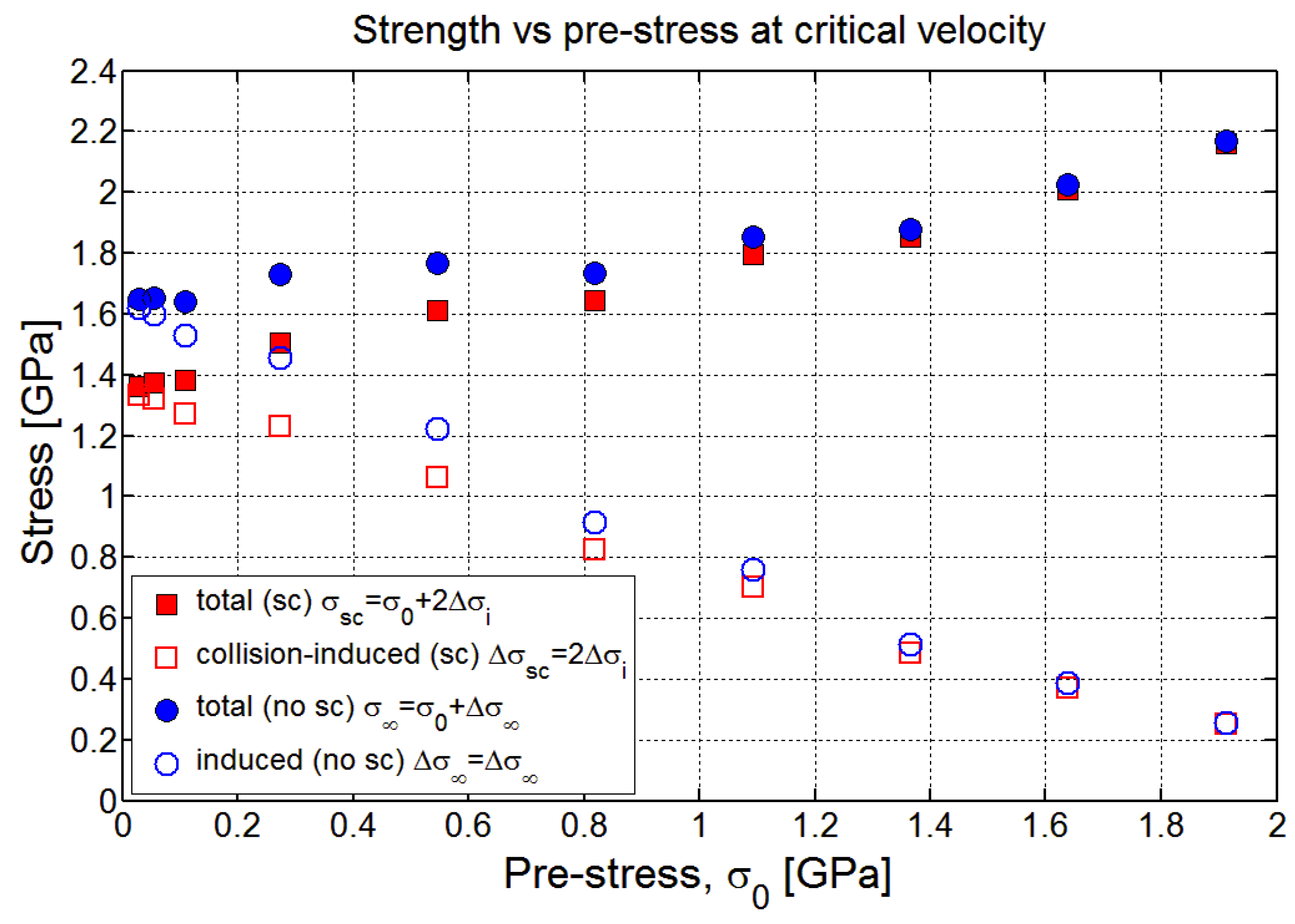[16] also noted a corresponding 23% and 17% increase, respectively, in these modulus values when preloads were increased from 54 to 658 MPa and 32 to 478 MPa, respectively. These authors interpreted this modulus increase with pretension as implying that the fiber has a non-linear stress-strain curve, yet the effect of impact velocity on modulus (i.e., through the tensile wave-speed) appeared to be negligible, which seems contradictory.

For the razor-edge impact experiments of Wang et al. [16], the extent to which the results yielded the strength of the two types of yarns is unclear, but the values quoted for Spectra^® 1000 and Kevlar^® were 715 MPa and 555 MPa, respectively, or about 1/5th the values found from quasi-static tension tests. At ballistic loading rates the fiber modulus values obtained were about half those obtained by Prevorsek et al. [20] and Field and Sun [27], though were consistent with the high strain-rate values obtained by Lim et al. [13]. Later on, Kavesh and Prevorsek [28] referred to an unpublished report wherein a Young’s modulus of 230 GPa was calculated from a directly measured, tensile wave-speed in Spectra^® fiber, though the exact version and level of pre-tension was not specified.

Carr [21] performed yarn shooting experiments on UHMWPE yarns (440 and 880 dtex Dyneema^® SK66) and aramid yarns (930 dtex Kevlar^® 129, 940 dtex Kevlar^® KM2, as well as 930 dtex Twaron CT yarns) where the main purpose was to investigate the failure modes during impact failure, rather than the critical velocity and yarn failure stresses. The projectile used was a steel sphere of mass 0.68 g and diameter 5.50 mm, and impact velocities ranged from 346 to 720 m/s. Note that the fully dense yarn diameters (viewed as one large cylindrical fiber without air spaces) were approximately 0.239 mm and 0.338 mm for the Dyneema^® SK66 yarns and 0.286 mm for the Kevlar^® and Twaron^® yarns, so accounting for roughly 80% packing of their filaments, these diameters would inflate by about 12% to 0.268, 0.378 and 0.320. These diameters are still more than an order of magnitude smaller than the projectile diameter.

Carr [21] characterized what she considered to be two distinct failure modes, the first being a transmitted stress wave (TSW) mode and the second being a shear failure mode, and the transition between the two modes was said to occur at impact energies (projectile kinetic energies) of 160 J and 130 J for UHMWPE and aramid yarns, respectively. Using the kinetic energy formula, $KE=m{V}^2/2$, such energies imply transition projectile velocities of 686 m/s for the Dyneema^® SK66 yarns and generally 618 m/s for the aramid yarns. An interesting feature associated with the so-called, high velocity shear mode was that a “shear plug” consisting of a finite length of yarn would be severed and then carried along by the projectile after failure. In the lower velocity TSW mode, the usual transverse triangle wave would be observed for a short time before yarn failure, which presumably was more distributed in nature, though not stated specifically beyond mentioning “gross permanent disruption of the yarn structure in all specimens for a distance of about 40 mm”, which is about 7 projectile diameters. The appearance of these two types of failure modes will be the subject of further discussion, but here it suffices to note that the existence of a severed shear plug counters the notion that a strain concentration naturally occurs at the midpoint of spherical contact.

Carr [21] noted another interesting phenomenon, namely that the energy absorbed during failure (measured from the decrease in projectile kinetic energy) versus impact velocity, had different trends in the two different fiber types. In the case of UHMWPE yarns, the specific energy absorbed in Joules/tex increased roughly linearly with projectile velocity, with no discernable jump or slope change at the transition velocity separating the failure modes. Exactly the opposite trend was noted for aramid yarns, namely a progressive decrease in absorbed specific energy with increasing impact velocity. This decrease accompanied reduced tendencies for both fibrillation and longitudinal splitting commonly observed in single aramid fibers, in favor of transverse fiber failure at higher velocities. In contrast, UHMWPE fibers exhibited no longitudinal splitting, but rather, the failure was said to be shear failure accompanied by shear bands in adjacent regions, as well as what was characterized in some cases as melt damage seen as a bulb of increased cross-sectional area over a fiber length of about three or four fiber diameters.

Bazhenov et al. [22] performed yarn shooting experiments on yarns of an aramid fiber called SVM (580 dtex) using a 3 cm diameter, hard spherical projectile, so about 100 times the yarn diameter. Experimentally, the critical velocity for yarn failure was reported to be 670 m/s. This was said to correspond to failure occurring nearly instantaneously but long enough after impact to establish a measurable deflection angle for the transverse wave of $\gamma \approx 31°$. Using the Rakhmatulin-Smith theory led to a predicted fiber strength value of 2.394 GPa. From their plot of quasi-static yarn stress-strain response, we confirm their Young’s modulus value of 114 GPa at strains below 1.5%, but also a tangent value of 80 GPa at strains approaching the failure strain (ignoring late stress roll-off in bundles due to load loss from random, Weibull-distributed, fiber failure strains). Bazhenov et al. [22] did not calculate a modulus value corresponding to the inferred tensile wave-speed from their tests. However, since the preload was small (said only to be enough to straighten the yarn), the Cole-Smith formulas in Prevorsek et al. [20] together with his V₀ value, 670 m/s, as well as the deflection angle, $31°$, results in a modulus value 115 GPa, so virtually identical to their 114 GPa quasi-static value.

Using arguments based on the effects of strain rate as predicted by the formula of Zhurkov [29], Bazhenov et al. [22] proposed that the relevant fiber strength in ballistic experiments should be at least 2.8 GPa (and based on single-filament composite tests a value as large as 3.3 GPa was even suggested). Accounting for nonlinear, finite strain effects, they used this value in their Rakhmatulin-Smith theory to predict a critical velocity of 770 m/s. This then led to attempts to explain the difference between the 670 m/s they observed, versus the 770 m/s they predicted.

In their first effort to explain this velocity difference, Bazhenov et al. [22] considered the influence of the observed nonlinearities in the stress-strain behavior of the fiber, but the resulting difference proved trivial. They then attempted an explanation in terms of a possible strain concentration generated by the spherical projectile shape during the growing contact and assuming a no-slip condition between the projectile and the yarn. Their initial analysis, based on discrete steps, led to a strain concentration of 2.62, obviously far larger than experimentally observed, and with further refinement of the steps, the stress concentration grew unbounded implying failure no matter how low the velocity of impact. This result obviously contradicted all published experimental data. Their result also contradicted theoretical results obtained by Rakhmatulin [8] for a similar geometry under frictionless slip (which would further increase the strain) whereby a spherical shape would begin with zero strain on first contact, followed by a progressive build up to the steady state value. Bhazhenov et al. [22] then attempted to revise their estimate of the strain concentration by invoking further non-linear effects, but still ended up with a significant stress concentration equivalent to ${\sec }^{2}31°=1.36$, which would reduce the critical velocity by the factor 1.26. Even this factor is considerably larger than their theoretical to experimental ratio 770/670 = 1.15.

Utomo and colleagues [23,24,25] performed yarn shooting experiments on Dyneema^® SK76 UHMWPE (1760 dtex) and Twaron^® (1760 dtex) yarns, and used a fixed 2.0 Kg weight to apply tension to the specimens. They used both an RCC flat-faced cylindrical projectile as well as a specially designed “saddle” projectile designed to capture the yarn (so it does not slide off the projectile nose) and to induce curvature in the yarn in the impact region, similar to that generated by a spherical projectile. They used the same theory as Prevorsek et al. [20] and calculated Young’s moduli of about 198 GPa and 135 GPa for their Dyneema^® SK76 and Twaron^® yarns, respectively, with limiting impact velocities said to be 485 m/s and 380 m/s, respectively. They did not, however, attempt to report yarn tensile strength results, possibly because of the obscuring effects of yarn fraying associated with having untwisted yarns. The moduli they calculated were said to be higher than the quasi-static values by factors of 1.5 and 1.3, respectively, but again, are much lower than those obtained by Prevorsek et al. [20] for materials of similar type.

Chocron et al. [30] have reported data from yarn shooting experiments involving 0.3 caliber, FSP projectiles impacting Kevlar^® S5705, Dyneema^® SK65 and Zylon^® PBO yarns. For a range of incremental impact velocities, it was determined whether or not yarns fail immediately by evaluating frames from high speed video. This gave ‘bracket’ values for the so-called critical threshold velocities causing yarn failure, which were lower than expected. Regarding the transverse wave speed, Smith’s theoretical predictions were compared with both experimental values and numerical values generated using LS-Dyna software using orthotropic continuum elements to model the yarn. A good match was found between the transverse wave speeds obtained by the three methods. The ability to accurately predict the transverse wave speed in impacted yarns is critical to being able to model impact into complex single and multi-layer woven systems for comparison to experiments.

Reasons for their lower-than-expected, transverse critical impact velocities causing yarn failure were discussed in a companion paper by Walker and Chocron [31]. (The paper acknowledges that this discrepancy was originally pointed out to the authors by van der Werff and Phoenix in 2010 including some discussion of the effect of strain doubling below a flat projectile having right-angle corners.) Walker and Chocron recast the classical theory in a rigorous form to derive that the strain in the yarn is uniform throughout the affected length also when the transverse wave passes. When a flat faced projectile strikes a yarn, they showed that the critical velocity is at least 11% lower than the classical solution predicts, when accounting for the effects of strain waves launched from the edges of the projectile that travel along the yarn inward and meet below the center of the projectile to double the strain. They proposed that, in addition, if the yarn were to ‘bounce off’ the projectile, the particle velocity would be doubled in the elastic case, and a potential 40% reduction of the critical impact velocity for yarn failure could be attributed to this effect. Such a bounce was seen in numerical modelling using the code, LS-Dyna, and was also experimentally reported by Field and Sun [27] in the case of a nylon sphere striking a rubber band. Additional details on yarn modeling can be found in Chocron et al. [32] who used four continuum elements for the yarn cross section and assumed a linear elastic, orthotropic constitutive model.

Advances in high speed photography have subsequently allowed very detailed observation of the yarn impact event as for instance in work by Song et al [33,34] for 450 denier Kevlar KM2 yarn where a Hopkinson bar was used for transverse impact testing. It is clearly visible that no bounce occurs, and additionally, non-uniform through-thickness compression of the yarn occurs before the back of the yarn begins to move. Further experimental observations by Hudspeth et al. [35], in the form of video footage of impacted Kevlar KM2 yarns, also showed yarns being squashed without bounce. Results presented by Hudspeth et al. in a series of papers [36,37,38], demonstrate that even in quasi-static transverse loading, an initial V-shaped angle causes a reduction in maximum transverse load for sharp indenters (razor blade and FSPs with small edge radius of curvature). This is attributed to a multi-axial, non-uniform stress state in the yarn, not accounted for in one-dimensional classical theory and variants. These works set the stage for involving non-homogenous, multi-axial stress states and wave interference effects to account for the reduction in critical velocity in yarn shooting experiments, as we later discuss and elaborate on in Appendix A.

Advances in numerical modeling have also resulted from specifically resolving a yarn into individual filaments, as was done by Nilakantan [39] who obtained a non-uniform stress state through the thickness and along the yarn under transverse impact. Sockalingam et al. [40] modeled the transverse impact of a single Kevlar^® KM2 fiber using a sufficient number of elements over the cross section to resolve a non-uniform stress state using a linear, orthotropic material model. A sensitivity study of the effect of the longitudinal shear moduli indicated that flexural waves next to the projectile are observed for increasing shear stiffness. Sockalingam et al. also showed that to model the quasi-static transverse compression of Kevlar^® KM2 [41,42] and Dyneema^® SK76 [43], it is crucial to include nonlinear inelastic behavior. If this approach is applied to transverse impact on 600 denier KM2 yarn with 400 individually modelled fibers (84 three-dimensional solid elements in the fiber cross section), a multi-axial stress state occurs with progressive loading through the thickness, as well as fiber squashing [44]. From the model, the predicted critical impact velocity (causing yarn failure) is about 500 m/s, while the classical value is over 900 m/s. The critical velocity is also sensitive to the longitudinal shear modulus where higher moduli result in lower velocities. In this case failure starts at the back of the curved fiber bundle.

1.4. Key Issues Arising from Study of Yarn Shooting Experiments in the Literature

From our study of the literature cited above, we list several important issues that arise, most of which we shall investigate later.

• Most studies report an increase in the effective fiber Young’s modulus at ballistic loading rates as compared to values calculated from quasi-static tension tests. However, the increase varied from almost none to an almost tripling of the quasi-static value.
• Studies of the effect on Young’s modulus of applying a steady yarn pre-tension prior to impact, were contradictory regarding the effect of increasing the yarn tension level.
• The tensile strengths calculated from yarn shooting experiments in the various studies fell short of quasi-static values by from 20% to as much as 80%.
• Though generally absent from the accepted 1-D theories of Rakhmatulin [7,8], Cole et al. [9] and Smith et al. [11], stress concentrations of some type appeared pervasive, depending on the type of projectile and even the yarn type and denier used.
• Energy absorbed by single yarns near the critical projectile impact velocity for yarn failure had very different trends for UHMWPE yarns versus aramid yarns, increasing with projectile velocity in the former and decreasing with projectile velocity in the latter.

1.5. Overview of the Paper

In Section 2, we begin by developing a 1D model for wave propagation in a thin, moderately-tensioned string subjected to transverse impact by a right circular cylinder (RCC) projectile of much larger transverse dimension. We assume the contact is frictionless, and upon impact, we model the evolution and collision in the center of tension waves emanating from the two edges, as well as subsequent wave interactions until the steady state is reached of propagating transverse and tension waves, asymptotically approaching the usually understood wave shape and stress profiles. We find that, shortly after impact, a significant strain concentration develops under the center of the projectile that depends on projectile impact velocity, and yarn pre-tension level, Young’s modulus, and linear density. We also determine initial versus steady state wave-speeds, angles, and material inflow (and outflow velocities). A schematic diagram is shown in Figure 2 of the various stages of wave reflection from the projectile edges towards the projectile center of contact, resulting in a limiting strain enhancement compared to point impact assumed in the classical, 1-D impact model of Figure 1.

In Section 3 we describe the yarn shooting experiments and experimental equipment used, including the two types of projectiles, and we discuss the various experimental results obtained. The experimental data consisted of both a sequence of high-speed, photographic images of the progressive growth of triangular transverse waves, and direct measurements of the tensile wave-speed using piezo-sensors. We discuss the observations showing that the critical impact velocity for yarn failure differs for the two projectile types, approaching 18% lower for the reversed FSP projectile vs. the saddle projectile under no yarn pre-tension. This translated into an apparent yarn tensile strength difference of almost 25% between the two projectile types.

In Section 4, we present various observations and plot the results using various frameworks of stress, strain, and critical velocity. We compare the results for the two projectiles to predictions from our theoretical model and the Cole-Smith model whose key formulas are presented in Appendix B. We also describe the effects of pre-tension and impact velocity on both the apparent yarn strength at the critical impact velocity and the modulus, as calculated from the measured tensile wave-speed. We discuss the extent to which the various measurements are self-consistent within the framework of the instantaneous elasticity assumptions in the model. This is followed by comparing the results to those appearing in the literature, and a discussion of any differences and reasons they occur.

In later subsections of Section 4, we discuss the phenomenon of a much lower calculated yarn strength at the critical velocity as compared to that measured in typical yarn tension tests. Appendix A proposes and develops a model to explain this difference in terms of fiber-to-fiber interference effects resulting from fiber transverse distortion and yarn compaction under and around the projectile from the transverse compressive shock wave.

Section 5 presents a summary of key observations and conclusions from the work. Appendix A provides details of the strain concentration from local yarn distortion under the projectile, and Appendix B provides the Cole-Smith formulas in our notation.

2. Analysis of the Impact of a Flat-Faced Projectile on a 1-D Yarn

The geometry of the flat-faced projectile problem is shown in Figure 2 along with several key quantities. The projectile is a flat-faced cylinder of diameter, $d_{\mathrm{p}}=2r_{\mathrm{p}}$, impacting a narrow string of width, $w_0$, depth, $h_0$, and where $d_{\mathrm{p}}\gg w_0\approx h_0>0$. The string may be a single fiber, or a yarn or a narrow string, and for convenience we let $A_0=w_0{h}_0$, be the effective fiber material cross-sectional area (ignoring voids and gaps between the fibers). We assume the contact between the projectile and string is frictionless. The mass, $M_{\mathrm{p}}$, of the projectile is assumed to be orders of magnitude larger than the mass of yarn directly in the projectile impact zone, and thus, the analysis is performed assuming a constant projectile velocity, $V$. Also, the string is under initial tension force, $T_0\ge 0$, prior to impact, where $T_0$ can range from zero to a large fraction of the string breaking strength, ${\sigma }_{\max ,0}{A}_0$.

We assume the material is very stiff in the longitudinal direction, and we let ${\mathsf{\epsilon }}_{\max ,0}$, be the failure strain, which is very small compared to unity. Thus, the overall induced strains, $\mathsf{\epsilon }$, will all be very small compared to unity, including the strain induced at tension, $T_0$. When we speak of quantities in terms of material coordinates, we mean that the quantities are referenced to the original longitudinal location, $r$, of a material point along the yarn before impact, where distance is measured from the central projectile axis. This distinction is particularly important when discussing transverse wave speed, whether in terms of the speed with respect to the original position of the material particles, called material coordinates, or with respect to the current location of the material points as viewed from the ground, called ground coordinates. Also, our analysis will describe behavior to the right of the main projectile axis since the behavior to the left can be determined from symmetry.

We shall consider changes in the geometry and the strain $\Delta \mathsf{\epsilon }$, relative to the equilibrium state at initial tension, $T_0$, which shall be the reference state for the material coordinate system (and where quantities have subscripts ‘0’, including $E_0$, and $A_0$). This viewpoint greatly simplifies the analysis, since before impact, the positions of points in material coordinates and ground coordinates are the same, irrespective of $T_0$, which would be held fixed throughout an impact experiment. We assume the material is linearly elastic, from the perspective of rapid changes in strain resulting from impact, and thus let $E_0$ be the material’s Young’s modulus measured with respect to near instantaneous, stress, and strain increases beyond those resulting from the initial tension, $T_0$. That is, $E_0$ can be viewed as the instantaneous tangent modulus at tension $T_0$, and as we shall see, may depend on the magnitude of $T_0$ through manifestation of nonlinear elastic and viscoelastic effects. Practically speaking, $E_0$ will be determined from the sonic modulus associated with the tensile wave induced by impact of the string, initially at tension $T_0$.

It is also convenient to define an effective elastic strain, ${\mathsf{\epsilon }}_0$, as ${\mathsf{\epsilon }}_0=T_0/\left(E_0{A}_0\right)$. Later we shall refer to ${\mathsf{\epsilon }}_{\max ,0}$ as the largest elastic strain the material can support, which will consist of the sum of ${\mathsf{\epsilon }}_0$ and the maximum possible additional elastic strain, ${\Delta \mathsf{\epsilon }}_{\max ,0}$, that the material can handle due to impact, also possibly dependent on $T_0$. Viewed in terms of the original un-tensioned material, the inherent equilibrium strain before impact is ${\epsilon }_{T_0}=T_0/\left(E_{T_0}{A}_0\right)$ where $E_{T_0}$ is a nominal secant modulus, possibly different from $E_0$, and is dependent on $T_0$.

If the strain resulting from the initial tension, $T_0$, is sufficient to significantly alter the linear density from the ‘as-manufactured’ condition, which would mean that $A_0=w_0{h}_0$ is no longer the as-manufactured cross-sectional area, then this will be accounted for in defining the pre-impact material state under initial tension, $T_0$. We mention this because various authors differ in what they consider to be the starting state just before impact, and thus, in how they account for the strain resulting from applying the initial tension, $T_0$. Also, the strains, ${\epsilon }_{T_0}$ and ${\epsilon }_0$ from initial tensioning may differ because of the previously mentioned non-linear, viscoelastic effects that occur over longer time scales, and that could become involved in strain changes from impact because of their effects on $E_{T_0}$. Such differences may relate mainly to the additional strain that can be absorbed upon impact, without causing failure of the material.

We summarize key quantities and their important attributes as follows: (i) the Young’s modulus, $E_0$, which is taken as fixed in terms of sudden changes in strain due to ballistic impact into the string under initial tension, $T_0$; (ii) the maximum elastic strain capability, ${\mathsf{\epsilon }}_{\max ,0}$, which is made up of the elastic strain ${\mathsf{\epsilon }}_0$ and any additional elastic strain, ${\Delta \mathsf{\epsilon }}_{\max ,0}$, that the material can support from projectile impact (also possibly dependent on $T_0$); and (iii) the total strain, ${\mathsf{\epsilon }}_{\max }$, the material can support from a tension test at low strain rates, which may be larger than ${\mathsf{\epsilon }}_{\max ,0}$, and also associated with nonlinear viscoelastic effects observable from changing the strain rate in a tension test.

We let ${\rho }_0$ be the density of the string material in the stretched state at tension, $T_0$, and for purposes of analyzing its ballistic response, the string is assumed linearly elastic with tensile wave-speed $a_0=\sqrt{E_0/{\rho }_0}$. Generally, we denote $\tilde{c}$ and $c$ as the transverse wave-speeds measured, respectively, relative to ground (called ground coordinates) and relative to the moving material (called material coordinates). Also, we denote $\Delta \mathsf{\epsilon }$ as the longitudinal strain induced in the string due to impact, and denote $\dot{u}$ as the velocity of the moving material particles as measured in ground coordinates.

The velocity, $\dot{u}$, is sometimes referred to as the ‘inflow velocity’ of string material that occurs behind the outward propagating tensile wave-front, but in the current context it will also refer to outflow of string material from under the projectile, which occurs for a brief period after impact (illustrated in Figure 2). These two material flow velocities are crucial to providing the extra length that allows a transverse wave-front to develop, whereby the string segment behind the front can form a large angle, $\gamma$, (~30°) with respect to the original horizontal string axis. These velocities will have various subscripts affixed to them, depending on the various states and time regions that occur.

2.1. Strain Immediately Following Impact

Immediately following impact and over the short time range, $0<t<r_{\mathrm{p}}/a_0$, two tensile wave fronts emerge from the projectile edge at position, $r_{\mathrm{p}}$, one traveling outward away from the projectile, and the other travelling inward under the projectile towards the projectile axis. We let

$$L_0^{(\pm )}=r_{\mathrm{p}}\pm a_{0}t$$

(5)

be the respective locations (outward and inward), in material coordinates, of the two wave-fronts up to the time, $t_{\mathrm{p}}=r_{\mathrm{p}}/a_0$, whereby the interior wave has traveled to the projectile center (See the first frame of Figure 2). Note that the total length of material traversed by the two tension waves is $2a_{0}t$, which differs from the case of no slip under the projectile whereby only one traversed length, $a_{0}t$, occurs due to the outward propagating tension wave.

Under constant projectile velocity the transverse deflection grows as

$$\delta =Vt$$

(6)

and for an initial, short time-period, the speed of the transverse wave front with respect to ground is denoted, ${\tilde{c}}_{\mathrm{i}}$, and is constant in time. (We affix the subscript ‘i’ to distinguish the values of certain quantities during this initial time-period before significant wave reflections occur.) The wave-front position, measured horizontally with respect to the main projectile axis, is

$$l_{\mathrm{i}}\left(t\right)={\tilde{c}}_{\mathrm{i}}t+r_{\mathrm{p}}$$

(7)

The initial cone angle (deflected yarn angle relative to horizontal) follows

$$\tan {\gamma }_{\mathrm{i}}=V/{\tilde{c}}_{\mathrm{i}}$$

(8)

so that

$$\sin {\gamma }_{\mathrm{i}}=V/\sqrt{{\tilde{c}}_{\mathrm{i}}^2+V^2}$$

(9)

The change in material length due to the two tension waves propagating from the projectile edge is determined from the geometry as

$$\Delta l_{\mathrm{i}}=\sqrt{{\left(l_{\mathrm{i}}-r_{\mathrm{p}}\right)}^2+{\delta }^2}-\left(l_{\mathrm{i}}-r_{\mathrm{p}}\right)=\sqrt{{\left({\tilde{c}}_{\mathrm{i}}t\right)}^2+{\left(Vt\right)}^2}-{\tilde{c}}_{\mathrm{i}}t$$

(10)

The strain increment (additional strain beyond that caused by initial tension, $T_0$), denoted $\Delta {\epsilon }_{\mathrm{i}}$, is calculated from this geometry as

$$\Delta {\epsilon }_{\mathrm{i}}=\frac{\Delta l_{\mathrm{i}}}{L_0^{(+)}-L_0^{(-)}}=\frac{\sqrt{{\tilde{c}}_{\mathrm{i}}^2+V^2}-{\tilde{c}}_{\mathrm{i}}}{2a_0}$$

(11)

Due to the outward propagating tension wave, the material inflow velocity behind the tensile wave-front at $L_0^{(+)}$ is given by

$${\dot{u}}_{\mathrm{i}}^{(+)}=-a_0\Delta {\epsilon }_{\mathrm{i}}$$

(12)

and similarly, due to the tension wave propagating inward under the projectile, the material inflow velocity (outflow, in fact) occurring to the right of the tensile wave-front at $L_0^{(-)}$ is

$${\dot{u}}_{\mathrm{i}}^{(-)}=a_0\Delta {\epsilon }_{\mathrm{i}}$$

(13)

(see Figure 2). Outside the projectile contact area, the velocities, $c_{\mathrm{i}}$, ${\tilde{c}}_{\mathrm{i}}$ and ${\dot{u}}_{\mathrm{i}}^{(+)}$ are related by

$${\tilde{c}}_{\mathrm{i}}=c_{\mathrm{i}}\left(1+\Delta {\epsilon }_{\mathrm{i}}\right)+{\dot{u}}_{\mathrm{i}}^{(+)}=c_{\mathrm{i}}\left(1+\Delta {\epsilon }_{\mathrm{i}}\right)-a_0\Delta {\epsilon }_{\mathrm{i}}$$

(14)

where the factor $\left(1+\Delta {\epsilon }_{\mathrm{i}}\right)$, in the first term on the right-hand side, accounts for the fact that the transverse wave is traveling in stretched material, and the second term accounts for the inflow motion of this stretched material. We shall retain the factor $\left(1+\Delta {\epsilon }_{\mathrm{i}}\right)$ but should note that $0<{\Delta \mathsf{\epsilon }}_i\ll 1$ (often less than 0.001) so it could be neglected with little loss in accuracy.

To solve for the accompanying strains, we must calculate the transverse wave-speed, that is, the speed of movement of the point where the string has a kink. For this purpose, we use the analogy of a thin belt travelling over a pulley of radius, $\stackrel{⌢}{r}$, and at relative velocity, ${\tilde{c}}_{\mathrm{i}}-{\dot{u}}_{\mathrm{i}}^{(+)}=c_{\mathrm{i}}\left(1+\Delta {\epsilon }_{\mathrm{i}}\right)$ with respect to the pulley center, as is discussed in Porwal and Phoenix [45] and Phoenix et al. [46]. (This velocity reflects the fact that the center of the pulley is moving at velocity ${\tilde{c}}_{\mathrm{i}}$ with respect to ground, whereas the material is moving at velocity ${\dot{u}}_{\mathrm{i}}^{(+)}$ with respect to ground, so the second must be subtracted from the first to obtain the relative speed at which material passes over the pulley.) The belt tension is given by

$$T_0+\Delta T_{\mathrm{i}}=T_0+h_0{w}_0{E}_0\Delta {\epsilon }_{\mathrm{i}}$$

(15)

and on a small element of belt within swept pulley angle, $d\theta$, and having contact force, $N$, per unit length against the virtual pulley, force balance dictates that

$$\left(T_0+\Delta T_{\mathrm{i}}\right)d\theta =N\stackrel{⌢}{r}d\theta +\left(\frac{{\rho }_0}{1+\Delta {\epsilon }_{\mathrm{i}}}\right)h_0{w}_{0}d\theta c_{\mathrm{i}}^2{\left(1+\Delta {\epsilon }_{\mathrm{i}}\right)}^2$$

(16)

The last term above is the string element mass times its centripetal acceleration, which also accommodates a small decrease in the belt linear density due to stretching by $\Delta {\epsilon }_0$. To have no net contact force on the pulley (since there is no physical pulley), we must have

$$N\stackrel{⌢}{r}=0$$

(17)

and using Equation (17) in Equation (16) and cancelling $d\theta$ and other quantities, we get

$$E_0\left({\epsilon }_0+\Delta {\epsilon }_{\mathrm{i}}\right)={\rho }_0{c}_{\mathrm{i}}^2\left(1+\Delta {\epsilon }_{\mathrm{i}}\right)$$

(18)

Using the definition of $a_0$, we rearrange Equation (18) to obtain

$$c_{\mathrm{i}}=a_0\sqrt{\frac{{\epsilon }_0+\Delta {\epsilon }_{\mathrm{i}}}{1+\Delta {\epsilon }_{\mathrm{i}}}}$$

(19)

Letting

$${\epsilon }_{\mathrm{i}}={\epsilon }_0+\Delta {\epsilon }_{\mathrm{i}}$$

(20)

be the virtual total strain in this time-period immediately after impact we rewrite Equation (19) as

$$c_{\mathrm{i}}=a_0\sqrt{\frac{{\epsilon }_{\mathrm{i}}}{1+{\epsilon }_{\mathrm{i}}-{\epsilon }_0}}$$

(21)

To calculate the strains, ${\epsilon }_{\mathrm{i}}$ and $\Delta {\epsilon }_{\mathrm{i}}$ in the above expression, we must match the change in material length from inflow and stretching, to the geometry of the deformed string path induced by impact, as calculated in Equations (10) and (11). From Equations (11) and (14) we obtain

$$\Delta {\epsilon }_{\mathrm{i}}=\frac{\sqrt{{\left(c_{\mathrm{i}}\left(1+\Delta {\epsilon }_{\mathrm{i}}\right)-a_0\Delta {\epsilon }_{\mathrm{i}}\right)}^2+V^2}-c_{\mathrm{i}}\left(1+\Delta {\epsilon }_{\mathrm{i}}\right)+a_0\Delta {\epsilon }_{\mathrm{i}}}{2a_0}$$

(22)

which can be rearranged to give

$$c_{\mathrm{i}}\left(1+\Delta {\epsilon }_{\mathrm{i}}\right)+a_0\Delta {\epsilon }_{\mathrm{i}}=\sqrt{{\left(c_{\mathrm{i}}\left(1+\Delta {\epsilon }_{\mathrm{i}}\right)-a_0\Delta {\epsilon }_{\mathrm{i}}\right)}^2+V^2}$$

(23)

Squaring both sides of Equation (23) and further manipulating the result leads to

$$4a_0{c}_{\mathrm{i}}\Delta {\epsilon }_{\mathrm{i}}\left(1+\Delta {\epsilon }_{\mathrm{i}}\right)=V^2$$

(24)

Using Equations (20) and (21) we can rewrite Equation (24) as

$${\epsilon }_{\mathrm{i}}{\left({\epsilon }_{\mathrm{i}}-{\epsilon }_0\right)}^2\left(1+{\epsilon }_{\mathrm{i}}-{\epsilon }_0\right)={\left(V/\left(2a_0\right)\right)}^4$$

(25)

Unfortunately the resulting equation is an implicit expression in ${\epsilon }_{\mathrm{i}}$, and furthermore, $\Delta {\epsilon }_{\mathrm{i}}$ and ${\epsilon }_{\mathrm{i}}$ may be of the same order of magnitude (due to ${\epsilon }_0$), i.e., in some cases ${\epsilon }_{\mathrm{i}}$ may be only a small multiple of ${\epsilon }_0$. This suggests a numerical solution may be necessary to guarantee high accuracy. However, an iterative approach can also be used resulting in a highly accurate closed-form solution after only a few steps.

From Equation (20) we have $\Delta {\epsilon }_{\mathrm{i}}={\epsilon }_{\mathrm{i}}-{\epsilon }_0$, and Equation (25) can be rewritten as

$$\left(\Delta {\epsilon }_{\mathrm{i}}\right)\sqrt{\left({\epsilon }_0+\Delta {\epsilon }_{\mathrm{i}}\right)\left(1+\Delta {\epsilon }_{\mathrm{i}}\right)}={\left(V/\left(2a_0\right)\right)}^2$$

(26)

Factoring out $\Delta {\epsilon }_{\mathrm{i}}$ from under the square-root leads to

$${\left(\Delta {\epsilon }_{\mathrm{i}}\right)}^{3/2}=\frac{{\left(V/\left(2a_0\right)\right)}^2}{\sqrt{\left(1+{\epsilon }_0/\Delta {\epsilon }_{\mathrm{i}}\right)}\sqrt{\left(1+\Delta {\epsilon }_{\mathrm{i}}\right)}}$$

(27)

We can expect both the cases $0<{\Delta \mathsf{\epsilon }}_i\ll 1$ and $0<{\Delta \mathsf{\epsilon }}_0\ll 1$. If the tension, $T_0$, is small and the impact velocity substantial, then we will have $0\le {\mathsf{\epsilon }}_0\ll {\Delta \mathsf{\epsilon }}_i$ and a good first approximation will be

$$\Delta {\epsilon }_{\mathrm{i}}\approx {\left(V/\left(2a_0\right)\right)}^{4/3}, 0\le {\epsilon }_0\ll \Delta {\epsilon }_{\mathrm{i}}$$

(28)

On the other hand, if the tension, $T_0$, is large and approaching the breaking strength of the yarn, then little additional strain can be accommodated from impact and we will have $0<{\Delta \mathsf{\epsilon }}_i\ll {\mathsf{\epsilon }}_0$. This forces the denominator in Equation (27) to grow unbounded, and considering the most dominant terms in an asymptotic analysis shows that a good first approximation is

$$\Delta {\epsilon }_{\mathrm{i}}\approx {\left(V/\left(2a_0\right)\right)}^2/\sqrt{{\epsilon }_0}$$

(29)

Thus, we have described the extremes of two regimes, but we desire an approximation that will work when ${\epsilon }_0$ and $\Delta {\epsilon }_{\mathrm{i}}$ are of roughly the same magnitude. As a first approximation to $\Delta {\epsilon }_{\mathrm{i}}$, for both regimes, and the transition in between we can use

$$\Delta {\epsilon }_{\mathrm{i}}\approx g_1\left(V/\left(2a_0\right),{\epsilon }_0\right)$$

(30)

where $g_1\left(\eta ,\zeta \right)$ is a function of two variables, $\eta >0$ and $\zeta >0$, and is given by

$$g_1\left(\eta ,\zeta \right)\equiv \min \left(1,\frac{1}{\sqrt{\zeta }}{\left(\eta \right)}^{2/3}\right){\left(\eta \right)}^{4/3}$$

(31)

Substituting this first general approximation, Equation (30), into the right-hand side of Equation (27) gives a second, more accurate approximation

$$\Delta {\epsilon }_{\mathrm{i}}\approx g_2\left(V/\left(2a_0\right),{\epsilon }_0\right)$$

(32)

where this second function is

$$g_2\left(\eta ,\zeta \right)=\frac{{\left(\eta \right)}^{4/3}}{{\left(1+\zeta /g_1\left(\eta ,\zeta \right)\right)}^{1/3}{\left(1+g_1\left(\eta ,\zeta \right)\right)}^{1/3}}$$

(33)

It turns out that one further iteration results in a highly accurate approximation, which is

$$\Delta {\epsilon }_{\mathrm{i}}\approx g_3\left(V/\left(2a_0\right),{\epsilon }_0\right)$$

(34)

where this third function is

$$g_3\left(\eta ,\zeta \right)=\frac{{\left(\eta \right)}^{4/3}}{{\left(1+\zeta /g_2\left(\eta ,\zeta \right)\right)}^{1/3}{\left(1+g_2\left(\eta ,\zeta \right)\right)}^{1/3}}$$

(35)

Finally, we have

$${\epsilon }_{\mathrm{i}}=\frac{T_0}{E_0{A}_0}+\Delta {\epsilon }_{\mathrm{i}}$$

(36)

One other important quantity is the tangent of the transverse wave angle, which from Equations (8), (14) and (19) can be written as

$$\tan {\gamma }_{\mathrm{i}}=\frac{V/a_0}{\sqrt{\Delta {\epsilon }_{\mathrm{i}}}\sqrt{\left(1+{\epsilon }_0/\Delta {\epsilon }_{\mathrm{i}}\right)}\sqrt{\left(1+\Delta {\epsilon }_{\mathrm{i}}\right)}-\Delta {\epsilon }_{\mathrm{i}}}$$

(37)

and using Equation (27) we obtain

$$\tan {\gamma }_{\mathrm{i}}=\frac{V/a_0}{{\left(V/a_0\right)}^2/\left(4\Delta {\epsilon }_{\mathrm{i}}\right)-\Delta {\epsilon }_{\mathrm{i}}}=\frac{4\left(V/a_0\right)\Delta {\epsilon }_{\mathrm{i}}}{{\left(V/a_0\right)}^2-4{\left(\Delta {\epsilon }_{\mathrm{i}}\right)}^2}$$

(38)

where we can use Equation (34) for $\Delta {\epsilon }_{\mathrm{i}}$.

As we shall discover, as soon as $t$ reaches $t_{\mathrm{p}}$, the opposing tension waves emanating from the two edges of the projectile (with associated strain increments, $\Delta {\epsilon }_{\mathrm{i}}$) collide underneath at the middle of the projectile. At that point, they spawn a symmetrically expanding tension wave wherein the strain amplitude is increased to ${\epsilon }_{\mathrm{SC}}={\epsilon }_0+2\Delta {\epsilon }_{\mathrm{i}}$, which constitutes a strain concentration compared to the initial value, ${\epsilon }_{\mathrm{i}}={\epsilon }_0+\Delta {\epsilon }_{\mathrm{i}}$, and a doubling of the incremental strain component to $2\Delta {\epsilon }_{\mathrm{i}}$. This expanding tension wave continues into the time range spanning $t_{\mathrm{p}}\le t\le 2t_{\mathrm{p}}$.

Before discussing the details of this important strain concentration effect, and to have a reasonable strain value to compare to, we must first consider the longer term asymptotic behavior of both the strain around the projectile and wave propagation, which is needed to assess the ultimate severity of the strain concentration relative to strains occurring in classical models of the problem. This strain is the same as when no slip is allowed under the projectile.

2.2. Strain at Long Times

The above analysis can be repeated for long times, $t\gg 2r_{\mathrm{p}}/a_0$, to determine the strain in the steady state, particularly in the projectile vicinity. The main departure from the analysis in the previous subsection is that in forming the growing, off-angle segment of the transverse wave, only the length up to the propagating tension wave-front, and inflow of material behind it, matters since the initial transient out-flow of material from under the projectile ultimately contributes negligibly to the growth of the transverse wave triangle. Thus, the analysis is similar to that for the case of no slip under the projectile. Throughout this section, we affix the subscript ‘$\infty$’ to differentiate these long-term quantities from the initial ones in the time period immediately after impact, which had subscript, ‘i’. We will give only the details where key differences in the mathematical structure occur. In analogy to Equation (20) we let

$${\epsilon }_{\infty }={\epsilon }_0+\Delta {\epsilon }_{\infty }$$

(39)

The first departure from the previous analysis is that Equation (11) is altered whereby the strain calculated from the geometry becomes

$$\Delta {\epsilon }_{\infty }=\frac{\sqrt{{\tilde{c}}_{\infty }^2+V^2}-{\tilde{c}}_{\infty }}{a_0},t\gg 2r_{\mathrm{p}}/a_0$$

(40)

and thus, is missing the factor, 2, in the denominator. Otherwise the pulley analogy, Equation (18), is the same, and the mathematical forms Equations (19) and (21) still apply for the transverse wave velocity, written in this case as

$$c_{\infty }=a_0\sqrt{\frac{{\epsilon }_{\infty }}{1+{\epsilon }_{\infty }-{\epsilon }_0}}=a_0\sqrt{\frac{{\epsilon }_{\infty }}{1+\Delta {\epsilon }_{\infty }}}$$

(41)

Also, the inflow velocity behind the tensile wave front is now

$${\dot{u}}_{\infty }=-a_0\Delta {\epsilon }_{\infty }$$

(42)

and the flow from under the projectile has stopped. Thus, we have

$${\tilde{c}}_{\infty }=c_{\infty }\left(1+\Delta {\epsilon }_{\infty }\right)+{\dot{u}}_{\infty }=c_{\infty }\left(1+\Delta {\epsilon }_{\infty }\right)-a_0\Delta {\epsilon }_{\infty }$$

(43)

To calculate the strain, we combine Equations (40) and (43) to obtain

$$\Delta {\epsilon }_{\infty }=\sqrt{{\left(\frac{c_{\infty }}{a_0}\left(1+\Delta {\epsilon }_{\infty }\right)-\Delta {\epsilon }_{\infty }\right)}^2+{\left(\frac{V}{a_0}\right)}^2}-\frac{c_{\infty }}{a_0}\left(1+\Delta {\epsilon }_{\infty }\right)+\Delta {\epsilon }_{\infty }$$

(44)

which can be rearranged to give

$$c_{\infty }\left(1+\Delta {\epsilon }_{\infty }\right)=\sqrt{{\left(c_{\infty }\left(1+\Delta {\epsilon }_{\infty }\right)-a_0\Delta {\epsilon }_{\infty }\right)}^2+V^2}$$

(45)

in analogy to Equation (23). Squaring both sides of Equation (45) and using Equation (41) with $\Delta {\epsilon }_{\infty }={\epsilon }_{\infty }-{\epsilon }_0$, we can rearrange the result to obtain

$$\left({\epsilon }_0+\Delta {\epsilon }_{\infty }\right){\left(\Delta {\epsilon }_{\infty }\right)}^2\left(1+\Delta {\epsilon }_{\infty }\right)={\left({\left(V/\left(\sqrt{2}{a}_0\right)\right)}^2+{\left(\Delta {\epsilon }_{\infty }\right)}^2/2\right)}^2$$

(46)

This result can be manipulated to yield

$$\Delta {\epsilon }_{\infty }=\frac{{\left[{\left(V/\left(\sqrt{2}{a}_0\right)\right)}^2+{\left(\Delta {\epsilon }_{\infty }\right)}^2/2\right]}^{2/3}}{{\left(1+{\epsilon }_0/\Delta {\epsilon }_{\infty }\right)}^{1/3}{\left(1+\Delta {\epsilon }_{\infty }\right)}^{1/3}}$$

(47)

Again, we have both $0<{\Delta \mathsf{\epsilon }}_{\infty }\ll 1$ and $0<{\mathsf{\epsilon }}_0\ll 1$, and once more we identify two limiting regimes of behavior. The first is $0\le {\mathsf{\epsilon }}_0\ll {\Delta \mathsf{\epsilon }}_{\infty }\ll 1$, in which case a first approximations is

$$\Delta {\epsilon }_{\infty }\approx {\left(V/\left(\sqrt{2}{a}_0\right)\right)}^{4/3}, 0\le {\epsilon }_0\ll \Delta {\epsilon }_{\infty }\ll 1$$

(48)

The second is ${\Delta \mathsf{\epsilon }}_{\infty }\ll {\mathsf{\epsilon }}_0\ll 1$, in which case we obtain the approximation

$$\Delta {\epsilon }_{\infty }\approx \frac{{\left(V/\left(\sqrt{2}{a}_0\right)\right)}^2+{\left(\Delta {\epsilon }_{\infty }\right)}^2/2}{\sqrt{{\epsilon }_0}}$$

(49)

If ${\epsilon }_0$ is close to the breaking strain, ${\epsilon }_{\max ,0}$, then $\Delta {\epsilon }_{\infty }$ must decrease to the point where it can be neglected in the numerator on the right hand side of Equation (49), and we obtain

$$\Delta {\epsilon }_{\infty }\approx \frac{1}{\sqrt{{\epsilon }_0}}{\left(\frac{V}{\sqrt{2}{a}_0}\right)}^2, \Delta {\epsilon }_{\infty }\ll {\epsilon }_0\ll 1$$

(50)

As a first approximation to $\Delta {\epsilon }_{\infty }$ for both regimes, as well as the transition in between, we can use

$$\Delta {\epsilon }_{\infty }\approx g_{\infty ,1}\left(V/\left(\sqrt{2}{a}_0\right),{\epsilon }_0\right)$$

(51)

where $g_{\infty ,1}\left(\eta ,\zeta \right)$ is a function of two variables, $\eta >0$ and $\zeta >0$, and is given by

$$g_{\infty ,1}\left(\eta ,\zeta \right)=\min \left(1,\frac{1}{\sqrt{\zeta }}{\left(\eta \right)}^{2/3}\right){\left(\eta \right)}^{4/3}$$

(52)

and thus, $g_{\infty ,1}\left(\eta ,\zeta \right)$ itself is identical to Equation (31), but the quantity inserted for $\eta$ now contains $\sqrt{2}$ in its denominator instead of 2. Substituting this first general approximation, Equation (51), into the right-hand side of Equation (47) gives the more accurate approximation

$$\Delta {\epsilon }_{\infty }\approx g_{\infty ,2}\left(V/\left(\sqrt{2}{a}_0\right),{\epsilon }_0\right)$$

(53)

where

$$g_{\infty ,2}\left(\eta ,\zeta \right)=\frac{{\left({\eta }^2+{\left(g_{\infty ,1}\left(\eta ,\zeta \right)\right)}^2/2\right)}^{2/3}}{{\left(1+\zeta /g_{\infty ,1}\left(\eta ,\zeta \right)\right)}^{1/3}{\left(1+g_{\infty ,1}\left(\eta ,\zeta \right)\right)}^{1/3}}$$

(54)

One further iteration results in a highly accurate approximation, which is

$$\Delta {\epsilon }_{\infty }\approx g_{\infty ,3}\left(V/\left(\sqrt{2}{a}_0\right),{\epsilon }_0\right)$$

(55)

where

$$g_{\infty ,3}\left(\eta ,\zeta \right)=\frac{{\left({\eta }^2+{\left(g_{\infty ,2}\left(\eta ,\zeta \right)\right)}^2/2\right)}^{2/3}}{{\left(1+\zeta /g_{\infty ,2}\left(\eta ,\zeta \right)\right)}^{1/3}{\left(1+g_{\infty ,2}\left(\eta ,\zeta \right)\right)}^{1/3}}$$

(56)

Finally, we have

$${\epsilon }_{\infty }=\frac{T_0}{E_0{A}_0}+\Delta {\epsilon }_{\infty }$$

(57)

2.3. Transverse Wave Angle at Long Times

A related important quantity is the tangent of the transverse wave angle, which is

$$\tan {\gamma }_{\infty }={V/\tilde{c}}_{\infty }$$

(58)

which from Equations (39), (41) and (43) can be written as

$$\tan {\gamma }_{\infty }=\frac{V/a_0}{\sqrt{\Delta {\epsilon }_{\infty }}\sqrt{\left(1+{\epsilon }_0/\Delta {\epsilon }_{\infty }\right)}\sqrt{\left(1+\Delta {\epsilon }_{\infty }\right)}-\Delta {\epsilon }_{\infty }}$$

(59)

Using Equation (46) we obtain

$$\tan {\gamma }_{\infty }=\frac{V/a_0}{{\left(V/a_0\right)}^2/\left(2\Delta {\epsilon }_{\infty }\right)-\Delta {\epsilon }_{\infty }/2}=\frac{2\left(V/a_0\right)\Delta {\epsilon }_{\infty }}{{\left(V/a_0\right)}^2-{\left(\Delta {\epsilon }_{\infty }\right)}^2}$$

(60)

Note that the approximation for the initial strain jump, $\Delta {\epsilon }_{\mathrm{i}}$, in Equation (34) and the long- time strain jump, $\Delta {\epsilon }_{\infty }$, in Equation (55) are quite similar in form. The crucial difference, however, is that the first involves the quantity, ${\left(V/\left(2a_0\right)\right)}^{4/3}$, whereas the second involves ${\left(V/\left(\sqrt{2}{a}_0\right)\right)}^{4/3}$.

From our initial approximations, Equations (28) and (48), which are applicable when $T_0$ is small, the steady-state, strain increase post-impact, $\Delta {\epsilon }_{\infty }$, becomes enhanced approximately by the factor $2^{2/3}$ relative to the initial value, Δε_i, prior to wave collisions under the projectile. This means that the strain, $\Delta {\epsilon }_{\mathrm{i}}$ immediately after impact, and before tension waves clash under the projectile, is smaller than the eventual, steady state value, $\Delta {\epsilon }_{\infty }$. The situation is different for the short-acting, strain enhancement resulting from collision of tension waves under the projectile, as we consider next.

2.4. Strain Jumps Caused by the Collision of Edge-Emitted Tension Waves Traveling under the Projectile

We can now assess the strain concentrating effects resulting from the collision of tension waves emitted from the projectile edges immediately after impact, and traveling under the projectile towards its center of contact. These edge emitted waves from impact correspond to initial incremental elastic strains, $\Delta {\epsilon }_{\mathrm{i}}$, which are superimposed on to the initial steady strain, ${\epsilon }_0$, generated by the applied tension, $T_0$, as illustrated in the first (top) frame in Figure 2. Once the wave traveling left under the projectile from the right edge, and with incremental strain amplitude, $\Delta {\epsilon }_{\mathrm{i}}$, (and total strain ${\epsilon }_0+\Delta {\epsilon }_{\mathrm{i}}$) has traveled distance $r_{\mathrm{p}}$, it collides at the projectile center-line with the sister tension wave traveling to the right from the left projectile edge, also with incremental strain, $\Delta {\epsilon }_{\mathrm{i}}$. This collision occurs at time, $t_{\mathrm{p}}=r_{\mathrm{p}}/a_0$, and results in a sudden doubling of the incremental strain to the level $\Delta {\epsilon }_{\mathrm{SC}}=2\Delta {\epsilon }_{\mathrm{i}}$, and thus, total strain of

$${\epsilon }_{\mathrm{SC}}={\epsilon }_0+\Delta {\epsilon }_{\mathrm{SC}}$$

(61)

This wave collision spawns an enhanced symmetric tension wave of uniform incremental amplitude, $\Delta {\epsilon }_{\mathrm{SC}}$, with spreading speed $a_0$, in both directions away from the projectile axis. This is seen in the second frame of Figure 2, where it is noted that the particle velocity in the spawned wave is zero behind its wave-front. This spreading is complete by time $t_{\mathrm{SC}}\approx 2r_{\mathrm{p}}/a_0$, at which time the entire length of the string portion under the projectile is uniformly tensioned at strain ${\epsilon }_{\mathrm{SC}}$, and notably there is no further flow of yarn material out from underneath the projectile. The enhanced tension wave then continues into the string region outside the projectile for an additional, short time until it ‘catches up’ with transverse wave-front traveling initially at speed, $c_{\mathrm{i}}$, in material coordinates, since $a_0\gg c_{\mathrm{i}}$. This is illustrated in the third frame of Figure 2. (Since it has no effect on the main results, we ignore any effects of slight ‘overhang’ beyond the projectile edge of stretched string material, whose length at time $t_{\mathrm{SC}}$ now becomes $r_{\mathrm{p}}\left(1+{\epsilon }_{\mathrm{SC}}\right)$ rather than $r_{\mathrm{p}}$). The ‘catch-up’ time of the enhanced tension wave is calculated to be

$${\widehat{t}}_{\mathrm{cu}}=\frac{2r_{\mathrm{p}}}{a_0-c_{\mathrm{i}}}$$

(62)

Note that behind the enhanced tension wave-front traveling to the right and beyond the projectile edge, the horizontal component of material flow velocity in ground coordinates is also zero, just as it would have been if no slip had occurred in the first place. Also the vertical component of the material velocity (‘vertical’ means in the direction of travel of the projectile) is the same as the velocity of the projectile, V, unlike the situation up to time $t_{\mathrm{p}}=r_{\mathrm{p}}/a_0$, where material out-flow from under the projectile occurs at velocity, $a_0\Delta {\epsilon }_{\mathrm{i}}$, meaning that the vertical component of material velocity is slightly smaller than the projectile velocity by the amount, $a_0\Delta {\epsilon }_{\mathrm{i}}\tan {\gamma }_{\mathrm{i}}$. (The first and second frames of Figure 2 only illustrate the reduced horizontal velocity component).

Unlike at the corner at the projectile edge, which can exert a force along a line bisecting the angle, $\gamma$, the enhanced tension wave cannot propagate unabated across the transverse wave-front, without inducing a sudden jump in the transverse wave-front velocity, $c$, and a local angle, $\gamma$. The reason is that tension balance must occur on each side of the transverse wave-front after the tension wave passes. Thus, what actually occurs is a slight reduction in the tension wave amplitude continuing on to right of the transverse wave-front (and traveling at speed $a_0$ in the material), and a new tension wave increment of negative strain amplitude emitted to the left to add to the strain level ${\epsilon }_{\mathrm{SC}}$, such that the strains become balanced at the same value, ${\widehat{\epsilon }}_{\mathrm{cu}}={\epsilon }_0+\Delta {\widehat{\epsilon }}_{\mathrm{cu}}$, on each side of the transverse wave-front, where ${\epsilon }_{\mathrm{i}}<{\widehat{\epsilon }}_{\mathrm{cu}}<{\epsilon }_{\mathrm{SC}}$. This situation is illustrated in the fourth frame of Figure 2.

Also, associated with these tensile wave changes emitted behind and in front of the transverse wave front is a slight reduction in string angle to the new value, ${\widehat{\gamma }}_{\mathrm{cu}}$, which is caused by the jump in transverse wave velocity to ${\widehat{c}}_{\mathrm{cu}}$. This jump results from the increased tensile strain, ${\widehat{\epsilon }}_{\mathrm{cu}}$, compared to the previous value ${\epsilon }_{\mathrm{i}}$, before the enhanced tension wave caught up to the transverse wave front at time, ${\widehat{t}}_{\mathrm{cu}}$. This new angle is much closer to the long-time asymptotic angle, ${\gamma }_{\infty }$, and the new strain is much closer to the long-time asymptotic strain, ${\epsilon }_{\infty }$, and they would match them exactly if it was not for a growing region of slight material contraction (caused by the slight reduction in strain from ${\epsilon }_{\mathrm{SC}}$ to ${\widehat{\epsilon }}_{\mathrm{cu}}$) in the new incremental tension wave now traveling to the left of the transverse wave-front, back towards the projectile, and then under it. This returning tension wave also induces a very small equilibrating material flow velocity back towards and then under the projectile edge of magnitude, $a_0\left({\epsilon }_{\mathrm{SC}}-{\widehat{\epsilon }}_{\mathrm{cu}}\right)$, as shown in frames four and five of Figure 2.

The effects of this slight contraction are small and short lived, and in fact, smaller and smaller tensile wave reflections (with incremental strain adjustments) travel back and forth from under the center of the projectile, and also out to the moving transverse wave-front, until the long-time angle, ${\gamma }_{\infty }$, and long-time strain, ${\epsilon }_{\infty }$, are asymptotically reached, as discussed in the previous sub-section. It turns out that the convergence is very rapid, and the first transitional value, ${\widehat{\epsilon }}_{\mathrm{cu}}$, is very close in magnitude to ${\epsilon }_{\infty }$, as is ${\widehat{\gamma }}_{\mathrm{cu}}$ to ${\gamma }_{\infty }$. The sixth (and last) frame of Figure 2, indicates that the process is virtually complete after the second tensile wave collision under the projectile emits a spreading tensile wave that catches and passes the transverse wave front.

2.5. Strain Concentrations Arising from Tensile Wave Collision under the Projectile

We let $K_{\mathrm{SC}}$ be the strain concentration caused by tension wave collision under the projectile as compared to steady state behavior (assumed in yarn shooting experiments). From Equations (39) and (61) we have the manipulation

$$K_{\mathrm{SC}}=\frac{{\epsilon }_{\mathrm{SC}}}{{\epsilon }_{\infty }}=\frac{2\Delta {\epsilon }_{\mathrm{i}}+{\epsilon }_0}{\Delta {\epsilon }_{\infty }+{\epsilon }_0}=2\left(\frac{\Delta {\epsilon }_{\mathrm{i}}}{\Delta {\epsilon }_{\infty }}\right)\left(\frac{1+\left(1/2\right){\epsilon }_0/\Delta {\epsilon }_{\mathrm{i}}}{1+{\epsilon }_0/\Delta {\epsilon }_{\infty }}\right)$$

(63)

Using Equations (34) and (55) for $\Delta {\epsilon }_{\mathrm{i}}$ and $\Delta {\epsilon }_{\infty }$, respectively, we can rewrite (63) as

$$K_{\mathrm{SC}}\approx \sqrt[3]{2}\left[\frac{2^{2/3}{g}_3\left(V/\left(2a_0\right),{\epsilon }_0\right)}{g_{\infty ,3}\left(V/\left(\sqrt{2}{a}_0\right),{\epsilon }_0\right)}\right]\left[\frac{1+{\epsilon }_0/\left(2g_3\left(V/\left(2a_0\right),{\epsilon }_0\right)\right)}{1+{\epsilon }_0/g_{\infty ,3}\left(V/\left(\sqrt{2}{a}_0\right),{\epsilon }_0\right)}\right]$$

(64)

While the factor $\sqrt[3]{2}$ proves to be important, the other factors exert considerable influence for large initial tensions, $T_0$. However, when $T_0={\epsilon }_0=0$, as is typical in ballistic armor, then

$$K_{\mathrm{SC},T_0=0}\approx \sqrt[3]{2}\left(\frac{2^{2/3}{g}_3\left(V/\left(2a_0\right),0\right)}{g_{\infty ,3}\left(V/\left(\sqrt{2}{a}_0\right),0\right)}\right)$$

(65)

and $\Delta {\epsilon }_{\infty }$ is simply ${\epsilon }_{\infty }$. In this case we can already achieve high accuracy by using $g_2\left(\eta ,0\right)$ and $g_{\infty ,2}\left(\eta ,0\right)$ of Equations (33) and (54), respectively, in place of $g_3\left(\eta ,0\right)$ and $g_{\infty ,3}\left(\eta ,0\right)$, respectively, and also we note that $g_1\left(\eta ,0\right)=g_{\infty ,1}\left(\eta ,0\right)={\left(\eta \right)}^{4/3}$. Thus

$$g_2\left(\eta ,0\right)=\frac{{\eta }^{4/3}}{{\left(1+{\eta }^{4/3}\right)}^{1/3}}\approx {\eta }^{4/3}\left(1-\frac{1}{3}{\eta }^{4/3}\right)$$

(66)

and

$$g_{\infty ,2}\left(\eta ,0\right)=\frac{{\left({\eta }^2+\frac{1}{2}{\eta }^{8/3}\right)}^{2/3}}{{\left(1+{\eta }^{4/3}\right)}^{1/3}}\approx {\eta }^{4/3}\frac{1+\frac{1}{3}{\eta }^{2/3}}{1+\frac{1}{3}{\eta }^{4/3}}$$

(67)

Manipulation of Equation (65) using binomial approximations to first order yields

$$\begin{array}{ll}\frac{2^{2/3}{g}_2\left(V/\left(2a_0\right),0\right)}{g_{\infty ,2}\left(V/\left(\sqrt{2}{a}_0\right),0\right)}& \approx \frac{2^{2/3}{\left(V/\left(2a_0\right)\right)}^{4/3}}{{\left(V/\left(\sqrt{2}{a}_0\right)\right)}^{4/3}}\frac{\left(1-\frac{1}{3}{\left(V/\left(2a_0\right)\right)}^{4/3}\right)\left(1+\frac{1}{3}{\left(V/\left(\sqrt{2}{a}_0\right)\right)}^{4/3}\right)}{1+\frac{1}{3}{\left(V/\left(\sqrt{2}{a}_0\right)\right)}^{2/3}}\\ & \approx 1-\frac{1}{3}{\left(V/\left(2a_0\right)\right)}^{4/3}+\frac{1}{3}{\left(V/\left(\sqrt{2}{a}_0\right)\right)}^{4/3}-\frac{1}{3}{\left(V/\left(\sqrt{2}{a}_0\right)\right)}^{2/3}\\ & \approx 1+\left(\frac{2^{2/3}-1}{3}\right){\left(\frac{V}{2a_0}\right)}^{4/3}-\frac{2^{1/3}}{3}{\left(\frac{V}{2a_0}\right)}^{2/3}\end{array}$$

(68)

and thus

$$K_{\mathrm{SC},T_0=0}\approx \sqrt[3]{2}\left(1+\left(\frac{2^{2/3}-1}{3}\right){\left(\frac{V}{2a_0}\right)}^{4/3}-\frac{2^{1/3}}{3}{\left(\frac{V}{2a_0}\right)}^{2/3}\right)$$

(69)

Typically, $V<a_0/20$ so that $V/\left(2a_0\right)<1/40$, and $\left(\left(2^{2/3}-1\right)/3\right){\left(1/40\right)}^{4/3}-\left(2^{1/3}/3\right){\left(1/40\right)}^{4/3}=-0.0322$. Hence $K_{\mathrm{SC},T_0=0}\approx \sqrt[3]{2}$ with an error of about 3%. Equation (69) and this last approximation are major results in the paper.

2.6. Penalty on Critical Failure Velocity Due to Strain Concentration from Wave Collision

Another way to view this result is to consider the effect of the strain concentration on the critical velocity for failure given the maximum strain capability, ${\epsilon }_{\max ,0}$, defined as

$${\epsilon }_{\max ,0}={\epsilon }_0+\Delta {\epsilon }_{\max ,0}$$

(70)

where $\Delta {\epsilon }_{\max ,0}$ is the maximum additional strain that the yarn material can handle without failure, given that it already supports elastic strain, ${\epsilon }_0$, associated with the applied tension, $T_0$. Then the maximum incremental strain must remain below

$${\epsilon }_{\max ,0}-{\epsilon }_0\approx 2\Delta {\epsilon }_{\mathrm{i}}\approx 2g_3\left(V/\left(2a_0\right),{\epsilon }_0\right)$$

(71)

whereas that ignoring the strain concentration from tension wave collision is

$${\epsilon }_{\max ,0}-{\epsilon }_0\approx \Delta {\epsilon }_{\mathrm{i}}\approx g_3\left(V/\left(\sqrt{2}{a}_0\right),{\epsilon }_0\right)$$

(72)

If we assume ${\epsilon }_0\ll {\epsilon }_{\max ,0}$ for calculating the maximum achievable velocities without failure, then using the methods above based on $g_2\left(\eta ,\zeta \right)$ and $g_{\infty ,2}\left(\eta ,\zeta \right)$, rather than on $g_3\left(\eta ,\zeta \right)$ and $g_{\infty ,3}\left(\eta ,\zeta \right)$, we can determine that

$${\epsilon }_{\max ,0}-{\epsilon }_0\approx 2{\left(\frac{V_{\mathrm{SC},\max }}{2a_0}\right)}^{4/3}\left(1-\frac{{\epsilon }_0}{3}{\left(\frac{2a_0}{V_{\mathrm{SC},\max }}\right)}^{4/3}\right)$$

(73)

based on a ${\epsilon }_{\mathrm{SC}}={\epsilon }_0+\Delta {\epsilon }_{\mathrm{SC}}={\epsilon }_{\max ,0}$, whereas

$${\epsilon }_{\max ,0}-{\epsilon }_0\approx {\left(\frac{V_{\max }}{\sqrt{2}{a}_0}\right)}^{4/3}\left(1-\frac{{\epsilon }_0}{3}{\left(\frac{\sqrt{2}{a}_0}{V_{\max }}\right)}^{4/3}\right)$$

(74)

based on ${\epsilon }_{\mathrm{i}}={\epsilon }_0+\Delta {\epsilon }_{\mathrm{i}}={\epsilon }_{\max ,0}$, where $V_{\mathrm{SC},\max }$ and $V_{\max }$ are the maximum achievable velocities with and without the strain concentration, respectively. Thus, for ${\epsilon }_0$ small, we have

$$V_{\mathrm{SC},\max }\approx \frac{\sqrt{2}{a}_0}{\sqrt[4]{2}}{\left({\epsilon }_{\max ,0}-{\epsilon }_0\right)}^{3/4}$$

(75)

corresponding to Equation (73), and

$$V_{\max }\approx \sqrt{2}{a}_0{\left({\epsilon }_{\max ,0}-{\epsilon }_0\right)}^{3/4}$$

(76)

corresponding to Equation (74). This tells us that the ratio of the two velocities is approximately

$$\frac{V_{\max }}{V_{\mathrm{SC},\max }}\approx \sqrt[4]{2}$$

(77)

also with error less than 3% for small ${\epsilon }_0$. This is also a major result in the paper. For the case $T_0={\epsilon }_0=0$, a somewhat similar approximation appeared in the paper by Walker and Chocron [31].

3. Experimental Apparatus, Materials, and Measurement Systems

3.1. Yarn Materials

Yarn shooting experiments were performed on UHMWPE Dyneema^® SK76 with material density ${\rho }_0=0.980\mathrm{g}/{\mathrm{cm}}^3$ (or $980\mathrm{kg}/{\mathrm{m}}^3$) and twisted to 40 turns per meter (tpm). The yarn had linear density, 1760 dtex, so the total cross-sectional area of the fibers in the yarn was 0.1796 mm². When fully compacted to a fiber volume fraction of 100%, the yarn would have an effective cylindrical diameter of 0.478 mm and outer-fiber helix angle of $3.44°$, whereas at 80% fiber volume fraction, the effective diameter is 0.534 mm and the helix angle to $3.85°$.

Twist was introduced into the yarns to provide sufficient coherence and resistance to fraying after impact, so that the transverse waves formed by yarns could be seen distinctly in multi-exposure photographs, and the failure event could be determined relatively unambiguously. This was particularly important for velocities approaching the critical velocity for yarn failure. Utomo and colleagues [23,24,25] had found previously that in untwisted Dyneema^® SK76 and Twaron^® aramid yarns, progressive fiber fraying could be seen in the growing transverse wave even at impact velocities more than 100 m/s below the critical velocity. The likely reason for the fraying is the existence of randomly distributed flaws along the individual filaments that results in both variability in their strengths and a reduction in strength with gage length, typically using Weibull statistics as discussed in Porwal et al. [47].

3.2. Reverse-Fired FSP and “Saddle” Nosed Projectiles

The projectile used in most of the experiments was a standard, cylindrical fragment simulating projectile (FSP) with a diameter of 5.385 mm, length of 6.35 mm and mass of 1.1 g. One end of an FSP is flat and the other has the shape of a flat-nosed chisel generated by symmetric $35°$ beveled flats shown in Figure 3. Contrary to convention, however, the typical projectile orientation in the gun barrel was reversed so that the flat end impacted the yarn, as would occur using an RCC. Some experiments also involved a “saddle” projectile, developed by Utomo and Broos [25] and also shown in Figure 3. This type of projectile was an RCC whose nose had been machined and polished to have a grooved channel cut into the nose forming a doubly-curved, saddle-shaped surface. The advantage was that, when properly oriented during impact, the yarn was guided into the groove so it could then progressively wrap around the nose of specific radius of curvature (approximately 3 mm, without sliding off to the side. The transverse width of the guiding groove at the base was 1 mm, so double the yarn diameter, but its radius of curvature was too mild to prevent yarn flattening.

3.3. Yarn Shooting Test Apparatus and Recording Equipment

The test apparatus consisted of a horizontally oriented, gas gun, firing transversely into the midpoint of a $L=4\mathrm{m}$ span of yarn horizontally stretched on a frame and aligned perpendicular to the gun barrel axis. Before projectile firing, the yarn was tensioned to a prescribed force using cylindrical capstans at each end, around which the yarn extremities were wrapped a few times before being tied down. One capstan was prevented from rotating and the wrapped yarn was knotted to a bolt on the frame. The capstan at the other end acted as smooth, cylindrical pulley that was free to rotate and had two, adjacent tie-down bolts embedded into the pulley surface to which one end of the wrapped yarn was tied. Load was applied to the rotating capstan cylinder using a rope that was wrapped around it and attached to the second bolt. A known mass was suspended from the other end of the rope and created a yarn tension equal to its mass times acceleration due to gravity (though for convenience of reporting the load magnitude we sometimes list the applied tensile load in units of kilograms). A schematic of the setup is shown in Figure 4. Touching the yarn, and located near the tied-down end, were two piezo-electric sensors (Pico miniatuur AE sensors with 400 kHz pre-amplifiers from PHYSICAL ACOUSTICS B.V., Rotterdam, The Netherlands) spaced a known distance, $d=1.2\mathrm{m}$, apart. These two sensors recorded the exact time of the passage of the longitudinal tensile wave. This is passage produces a sharp rise of the piezo-electric signal. From these signals, the times of passage of the tension wave emitted from the impact position, and based on the time-of-flight and distance, d, the tensile wave-speed, $a_0$, could be calculated. As shown in Figure 4, these were sufficiently far from the impact location to allow a transverse wave to grow along the yarn approximately 20 cm (40 cm total triangular span) before reaching the piezo sensors. Note that the tension wave typically traveled at a speed about ten times that of the transverse wave, so the free span of yarn had to be close to 10 times the span of observation of the transverse wave, i.e., the 4 m chosen, in order avoid interference due to wave reflections from the clamps.

At a sequence of closely spaced time intervals, the instantaneous location of the triangular transverse wave, with the projectile at its apex, was recorded using a multi-exposure camera with a flash exposure time of 500 ns. The camera typically superimposed 10 snapshot images on one photograph spaced in time so that the projectile traveled about 1 to 1.2 cm in between. For instance, at 400 m/s this was every 25 to 30 $\mathsf{\mu }\mathrm{s}$. From the photographed geometry of progression of the projectile and triangular transverse wave, the actual projectile velocity, speed of the transverse wave-front, and the angle formed by the yarn segment in between, could be calculated. Thus, the projectile and transverse wave could be observed for about 270 $\mathsf{\mu }\mathrm{s}$, which at 369 m/s or 0.369 $\mathrm{mm}/\mathsf{\mu }\mathrm{s}$ provided about 100 mm of projectile travel and roughly 200 mm of transverse wave-front travel (full span 400 mm), consistent with the overall yarn length, L of 4 m.

Projectiles were fired at velocities ranging from 150 m/s to 555 m/s into yarn specimens with tensions induced by suspended masses ranging from 0.535 kg to 40 kg, so well below the 63 kg breaking strength of the yarn as measured in a standard yarn tension test on 50 cm specimens. The corresponding range of tensile stress levels in the yarn were, 29.22 MPa to 2185 MPa compared to the breaking strength of 3440 MPa. Higher loads were impractical for two reasons: First, including capstan wrapping, the fully tensioned yarn length was 5 to 6 m, and before firing the projectile, the yarn had to be placed under tension for some time (a minute or two) to ensure precise alignment and stability of the experimental setup. Thus, both statistical size (length) effects and mild stress rupture effects meant that some yarns would fail before firing, if initially applied loads were 45 kg (2460 MPa) or higher.

At such high tensions, irrespective of yarn length, the critical impact velocity for failure was less than 140 m/s, making it more difficult to obtain accurate measurements from the photographs. It is important to note that stresses due to impact just below the various critical velocities for failure were measured effectively over a relatively short yarn length involving about 2 cm of projectile travel, 4 cm of transverse wave-front travel and 40 cm of tension wave travel. However, only fiber failures from the tension wave occurring within about 20 cm of the projectile could reflect back unloading waves to influence the fiber failure activity observed in the transverse wave, due to overloads imposed on surviving fibers. Thus, filament failures within a total length of up to 40 cm would play a role in determining the critical velocity for yarn failure especially for the saddle projectile. Of course, for the flat-nosed, reverse-fired FSP projectile, and just above its critical velocity, colliding of tension waves under the projectile, would occur virtually instantly (~0.1 $\mathsf{\mu }\mathrm{s}$).

4. Results and Observations from Yarn Shooting Experiments

Figure 5 shows three separate cases of a sequence of about 10 superimposed snapshots each (maximum possible is 16). In the middle frame, end-to-end projectile tumbling appears to have occurred, due perhaps to off-centered impact, thus causing the yarn to eventually slide off the flat cylinder nose. Interestingly this slip-off results in superposition of a traveling transverse wave of opposite sign causing cancellation of the yarn travel and a growing flat region expanding at the same speed as the progression of the transverse wave-front. Note also that the projectile mass is sufficiently large relative to the yarn mass for the deceleration of the projectile to be negligible over the time and distance of measurement.

Figure 6 plots results for tensile wave-speeds measured in Dyneema^® SK76 yarns under impact velocities ranging from 25 m/s to 550 m/s and tensile loads from 0.535 Kg to 40 Kg corresponding to fiber tensile stresses from 29.22 MPa to 2185 MPa. In each case, the results are for velocities ranging from the critical velocity to well below that value. Except perhaps at the very lowest load of 0.535 Kg, the tensile wave-speed measured was minimally influenced by the impact velocity by at most 5%.

4.1. Yarn Young’s Modulus Versus Pre-Stress and Impact Velocity

Using the formula $E_0=a_0^2{\rho }_0$, the results in Figure 6 were used to calculate the yarn Young’s moduli in Figure 7 associated with the various projectile impact velocities. The modulus values range from about 130 GPa at the lowest tensions (less than 1% of the breaking strength) to about 208 GPa at a tension corresponding to 40 Kg. Figure 8 shows the averaged modulus results from Figure 7.

Using the same Dyneema^® SK76 yarn with very little or no twist, under a load of 2.012 Kg, Utomo and Broos [25] reported a value of about 196 GPa. In our case, at a load of 2 kg the measured modulus is considerably lower at about 150 GPa, and to achieve 196 GPa requires a load in our case corresponding to 20 Kg. While the difference would seem to be the result of twist in the yarn (40 tpm vs. almost none), we must also note that our modulus values were calculated directly from the measured tensile wave speed, whereas the values of Utomo and Broos [25] were calculated indirectly from the tangent of the deflection angle (projectile velocity over transverse wave-speed in ground coordinates) using the Cole-Smith equations.

In view of this difference in calculated Young’s modulus, we repeated the experiments of Utomo and Broos [25] on 1680 dtex Twaron^® but using 40 tpm. Unlike the situation with Dyneema^® SK76, at a 2 Kg load we obtained a close but slightly higher value, 141 GPa, than their reported value of about 135 GPa, and interestingly this value is much larger than the value often quoted 90 GPa from standard tension tests. We note that, because of the difference in densities, the Twaron^® outer helix angle was significantly less than for the Dyneema^® SK76, making the twist effect smaller.

As mentioned, following the theory in the previous section, a second method for calculating the tensile wave-speed can be performed using the yarn deflection angle, ${\gamma }_{\infty }$, as in the Cole-Smith theory given in Appendix B. The calculation involves use of Equation (49) (or more easily Equations (55) and (56)) together with Equation (60) for ${\gamma }_{\infty }$, to solve for $a_0$, and then, the Young’s modulus can be calculated using $E_0=a_0^2{\rho }_0$. Alternatively we can calculate angle, ${\gamma }_{\infty }$, to expect from Equations (55), (56) and (60) using V, $T_0$, ${\rho }_0$, $A_0$, and the Young’s modulus value, $E_0=a_0^2{\rho }_0$, but calculated directly from $a_0$ measured from the piezo-electric sensors. As shown in Figure 9, the calculated values of ${\gamma }_{\infty }$ agree very closely with the measured values, whether the Cole-Smith method (Appendix B) or method described above is used, suggesting no significant discrepancy between the two methods and results measured.

As discussed in the Introduction, several studies involving yarn shooting experiments have appeared in the literature, looking at the ballistically relevant modulus of UHMWPE fibers and yarns, particularly Spectra^®. Prevorsek et al. [20] used photographic images of the growth of the transverse wave rather than directly measuring the tensile wave-speed. The various results for Young’s modulus obtained for UHMWPE fibers are summarized in Figure 10, and what singularly stands out is the very high tensile modulus for Spectra^® 1000 of about 310 GPa as was mentioned in the Introduction. This value is particularly puzzling in view of the much lower values obtained by Wang et al. [16], who apparently used the same material (and shared a common co-author). It might also be noted that the Prevorsek et al. [20] value of 225 GPa for Kevlar^®, which appears to have been either Kevlar^® 129 or Kevlar^® KM2, is far higher than the value 137 GPa obtained by Utomo and Broos [25] for a similar fiber Twaron^®, and the even lower value 122 GPa reported by Wang et al. [16] apparently for the same Kevlar^® used by Prevorsek et al. [20].

To understand this large discrepancy, we studied the one photograph provided by Prevorsek et al. [20], which showed a time sequence of the growth of the transverse wave around the projectile, whose image was clearly identifiable. Using special software to extract the wave angle, $\gamma$, as the projectile progressed we calculated the sequence of angles, $12.2°$, $12.2°$, $12.5°$, but then, the angles in the last two frames dropped to, $10.7°$ and $10.8°$. The projectile had a roughly spherical nose and its diameter and length were given as 24.3 mm and 34 mm, respectively, and the impact velocity was reported as 130 m/s. The preload tension used for this particular image sequence was not provided, but using their version of the Cole-Smith formulas (see Appendix B) with the four possible tensions in their Table III, these angles could only have corresponded to their lowest preload, 250 MPa, since otherwise the angles would have been much smaller. (This assessment was confirmed upon study of transverse wave-speed behavior observed in figures for other cases given in Field and Sun [27], who had provided preload values.) Using the formulas in Appendix B, their Young’s modulus of 310 GPa corresponds to an angle of $\gamma =10.9°$, and thus, we infer that Prevorsek et al. [20] must have used angles calculated from the last two frames (corresponding to our estimates of $10.7°$ and $10.8°$) to calculate the yarn Young’s modulus, and they ignored the three angles at earlier times, which average to $\gamma =12.3°$. The dimensions of the triangle wave were certainly largest in these last two frames, so the resolution might seem to be the best (and having only one photographic image is really all that is needed to calculate the yarn, Young’s modulus).

It was mentioned earlier that the calculated Young’s modulus is approximately proportional to $1/{\gamma }^6$, so a small change in angle corresponds to a large change in estimated yarn modulus. Our use of the angle $\gamma =12.3°$, results in a modulus close to our value for Dyneema^® SK76 for the same preload stress and the value obtained by Wang et al. [16] for the same material and preload stress. Prevorsek et al. [20] did not provide geometric details of the yarn specimens, especially their length, but they were suspended vertically with a clamp at one end and a hanging weight on the other. However, based on more extensive photograph sequences and figures provided in Field and Sun [27], which were not duplicates of those in Prevorsek et al. [20], we estimated that the upper clamp or guide restricted transverse motion approximately 10 cm above the impact point, which agrees with the value 0.1 m stated in the paper. The type of clamp was not described, so the potential for yarn slippage and attenuation of the tension jump upon reflection from the clamp could not be assessed (although the use of neoprene is indicated in their figure). At an impact velocity of 130 m/s, use of the last two photographic frames to determine the transverse wave angle (at about 100 $\mathsf{\mu }\mathrm{s}$ after impact) would require a gage length of about 1 m, impacted centrally, to avoid strain increases from tensile wave reflections from the extremities, which in turn would more than double the tension and lower the angle beginning at the transverse wave-front and progressing backwards. Avoiding this problem would require placing the upper clamp at 0.5 m above the impact point, so much more than the 0.1 m mentioned in the paper, and thus, yarn slippage could not mitigate the strain increases resulting from the implied multiple reflections of the tensile wave. These observations are provided to offer an explanation for the large discrepancy between the results of both Prevorsek et al. [20] and Field and Sun [27], and our measurements as well as those of Utomo and Broos [25] for Dyneema^® SK76 and also those of Wang et al. [16] for Spectra^® 1000.

4.2. Critical Velocity for Yarn Failure Versus Projectile Type and Yarn Pre-Stress Level

Figure 11 shows a plot of the measured critical impact velocity for yarn failure versus tensile pre-stress, both for the cylindrical, reverse-fired FSP projectile and the saddle projectile, and clearly there is a significant difference in critical velocity of about 18% between the two projectiles. We also show predictions of critical velocity resulting from theoretical removal of the strain concentrating effects of tensile wave collision under the flat face of the cylindrical projectile. That is, we calculate the critical velocities using Equations (55) and (56), except we replaced $\Delta {\epsilon }_0$ by $\Delta {\epsilon }_{\mathrm{i}}$ calculated from Equations (33) and (34) for the flat faced projectile. This correction results in critical velocities that are very close to the experimental critical velocities obtained using the saddle projectiles across the range of yarn initial loads for which saddle projectile experiments were run. The ratio of critical velocities at small initial tension (small ${\epsilon }_0$) also reveals about an 18% improvement upon removing the strain concentration. This difference is consistent with the approximate predicted ratio, $\sqrt[4]{2}=1.189$, from Equation (77). This difference in critical velocity translates to a strain concentration from the tensile wave collision of about 1.25, in agreement with the approximate value $\sqrt[3]{2}$ after Equation (69).

Note that the critical velocity, in Figure 11, linearly projects to zero at the quasi-static, yarn strength value of 3.4 GPa, as measured in standard tension tests. Measuring lower critical velocities at higher yarn pre-stresses was problematic because the long yarn specimens would often fail prematurely before shooting, for reasons stated earlier. Nevertheless, the pivotal yarn strength at zero impact velocity is the quasi-static yarn strength. This is understandable from the perspective that the failure process in yarn shooting experiments typically occurs over a relatively short length of yarn, earlier said to be at most 40 cm. This length is similar to gage lengths used in standard tension tests.

In the Introduction, we mentioned results by Rakhmatulin [8] that strongly suggest that a projectile with a rounded nose contacting the yarn will generate a gradually increasing tensile stress, mainly because the angle of the transverse wave itself, which is crucial to generating strain in the tension wave, can only build up gradually. This is described also in Rakhmatulin and Dem’yanov [15]. Thus, for most cylindrical projectiles with rounded nose shapes, there will be no tensile wave collision in the contact zone and thus no resulting strain concentration, unlike the case of a flat faced cylindrical projectile, or for any projectile that is flat but with a discontinuous change in angle at each edge larger than the transverse wave angle, ${\gamma }_{\infty }$, (e.g., an FSP). This aspect warrants further study.

4.3. Yarn Failure Stress and Strain at Critical Velocity Versus Tensile Pre-Stress

Figure 12 shows results for the yarn failure stress from impact as a function of yarn tensile pre-stress and associated critical velocity for yarn failure, as calculated directly from the experimental results for both the cylindrical projectile and the saddle projectile. Figure 13, shows calculated yarn strains associated with impact including the change in strain from the impact event and the strain induced from the pre-stress. While removal of the strain concentration by using saddle-shaped projectile helps to flatten the curve, there is still a strong tendency for a lower effective yarn failure stress at higher critical velocities, corresponding to low yarn pretension. Approaching zero yarn pre-stress, the apparent yarn strength at the critical impact velocity projects to about 1.7 GPa, which is about half that seen in standard tension tests and the projected value indicated in Figure 11.

Thus, while it has been possible to explain the critical velocity differences between the two projectile types in terms of stress concentration effects of tensile wave collision under a flat faced projectile, we are left with an observed strength difference at the highest critical velocities of about two. This situation is not unique to the UHMWPE Dyneema^® SK76 yarns tested here, but was also specifically noted in the experiments of Bazhenov et al. [22] on aramid yarns, and upon further study, is apparent also in most of the yarn shooting experiments mentioned above, whether using UHMWPE or aramid yarns.

Before proposing possible explanations for this unmistakable phenomenon, we revisit the observations made by Cunniff [5] in fabric shooting experiments on UHMWPE Spectra^® 1000 multi-layered fabrics. Cunniff [5] achieved V50 velocities that required a normalizing critical velocity of $V_{\mathrm{C}}=672\mathrm{m}/\mathrm{s}$. He originally assumed a yarn strength of ${\sigma }_{\max }=2.57\mathrm{GPa}$, a Young’s modulus $E=120\mathrm{GPa}$, and failure strain, ${\epsilon }_{\max }=0.0350$, (implying non-Hookean stress-strain behavior), and this resulted in $V_{\mathrm{C}}=801\mathrm{m}/\mathrm{s}$, which was too high in value. Using Equation (4) assuming the lower critical velocity $V_{\mathrm{C}}=672\mathrm{m}/s$ requires a lower tensile strength of ${\sigma }_{\max }=2.0\mathrm{GPa}$, assuming the same Young’s modulus, $E=120\mathrm{GPa}$, and scaled-back failure strain. Even this strength is higher than our experimental value of ${\sigma }_{\max }=1.70\mathrm{GPa}$ at zero pre-stress.

On the other hand, using ${\sigma }_{\max }=1.70\mathrm{GPa}$ and a Young’s modulus value of $E=130\mathrm{GPa}$, and assuming Hookean behavior, Cunniff’s formula predicts $V_{\mathrm{C}}=507\mathrm{m}/\mathrm{s}$, which is much below $611\mathrm{m}/\mathrm{s}$ projected from our saddle experiments at $T_0=0$ (although fortuitously similar to the value $513\mathrm{m}/\mathrm{s}$ from our reverse-fired, FSP yarn shooting experiments). Coincidentally, a yarn strength of ${\sigma }_{\max }=3.38\mathrm{GPa}$, and Young’s modulus, $E=130\mathrm{GPa}$, under Hookean assumptions, does result in $V_{\mathrm{C}}=801\mathrm{m}/\mathrm{s}$, using his Equation (4). Nonetheless significant discrepancies remain unexplained.

One difficulty in using Cunniff’s Equation (4) is that it is not fully consistent with the critical velocity predicted by the 1D-theory for yarn failure, irrespective of the version used. In our case, assuming zero pre-stress so that $\Delta {\epsilon }_{\infty }={\epsilon }_{\infty }$, and inverting Equation (48), the critical velocity is

$$V_{\mathrm{crit}}\approx \sqrt{2E/\rho }{\left({\sigma }_{\max }/E\right)}^{3/4}$$

(78)

Thus, as already previewed in Equation (4), we have

$$V_{\mathrm{crit}}=2^{5/6}{\epsilon }_{\max }^{1/12}{V}_{\mathrm{C}}$$

(79)

a sensitivity to strain noted also in Phoenix and Porwal [6] for a 2D membrane model.

For instance, assuming a strain to failure of 0.0130, which is the projected limiting value in Figure 13, we find that $V_{\mathrm{crit}}=1.24V_{\mathrm{C}}$, which shows that there is a significant difference between Cunniff’s critical normalizing velocity $V_{\mathrm{C}}$ and the theoretical critical velocity associated with 1D yarn impact. It is further interesting to note that, assuming ${\sigma }_{\max }=3.38\mathrm{GPa}$, Young’s modulus $E=130\mathrm{GPa}$, and Hookean stress-strain behavior, Equation (78) yields $V_{\mathrm{crit}}=1055\mathrm{m}/\mathrm{s}$, so considerably higher than the critical value of Cunniff [5]. Thus, irrespective of the theoretical method used to predict critical velocity and the type of yarn tested, the question remains as to why yarn shooting experiments give critical velocities and implied strengths much lower than predicted.

4.4. Strain Concentration from Impact and Shock Wave Distortion of the Yarn Cross-Section

For both the flat faced RCC projectile and the saddle projectile in Figure 3, the moderately twisted yarns of Dyneema^® SK76, said earlier to have diameter $h_0\approx 0.53\mathrm{mm}$ (with 20% air voids between fibers) before impact, are estimated to flatten under the projectile during impact to approximate dimensions of perhaps $h_{\mathrm{c}}\approx 0.25\mathrm{mm}$ and perhaps 1.00 mm width (i.e., approximately a rectangular cross-section with aspect ratio of 4 and slightly reduced void space—see Song et al. [34] for a demonstration of this phenomenon). The effective velocity of such a compressive shockwave, is not easy to calculate for such a complex transverse yarn structure with voids, but may well be of the order of 1200 m/s, so that compaction would be complete in perhaps in as little as $0.5\mathsf{\mu }\mathrm{s}$, though still long enough for the tension wave to travel 5 to 6 mm.

Outside the region of impact, however, the yarn cross-section would have a more circular (or mildly elliptical) shape, so for the fibers directly against the projectile, their stretched path lengths passing into and through the emerging transverse wave front must be longer than for those underneath and on the opposite side of the yarn furthest from projectile contact. Since the helical length of one turn of twist is about 2.5 cm, there will initially be a significant interference effect between the fibers. Fibers contacted first are at a higher deflection angle, $\gamma$, and thus, have more strained than others beneath at lower deflection angles, particularly since the induced tensile strain varies roughly as ${\gamma }^4$. Consequently, fibers underneath are simply in the way, in some respects acting as added mass to the fibers above, thus slowing down the transverse and tensile waves. Interference effects have been demonstrated experimentally by Cunniff [48] and theoretically by Porwal and Phoenix [45] and by Phoenix et al. [46], to result in a substantial reduction in the critical failure velocity of multi-layer, hybrid systems. Much the same phenomenon can be expected in yarns.

While a thorough experimental study of this phenomenon (which would benefit from various yarn sample modifications) is beyond the scope of the current paper, it is still a worthwhile exercise to outline a model that may explain the observed phenomenon, especially one that results in a high stress concentration under reasonable assumptions. Such a model has been developed in this paper, and in order not to detract from the paper’s main focus, it is described in Appendix A.

The model shows how a transverse compressive shock wave, and the local yarn and projectile geometries involved in typical yarn shooting experiments can result in transverse yarn compaction and strain concentrations of as much as two times the average tensile strains induced from impact. This may happen during the first fraction of a microsecond if the fibers directly in contact with the projectile travel at velocity V, whereas those deeper into the yarn under the projectile travel initially at a considerably lower velocity until yarn compaction is complete. This is precisely the situation noted by Song et al [33,34]. The reader is referred to Appendix A for theoretical details.

5. Conclusions

We have performed yarn shooting experiments on Dyneema^® SK76 twisted yarns with various pretension levels and using two types of projectiles, a flat-faced cylindrical projectile (reverse-fired FSP) and a special saddle-nosed projectile. Experimental data consisted of a time-sequence of high-speed, photo-images of the growth of the triangular transverse wave, as well as direct measurement of the tensile wave speed using two precisely-spaced, piezo-electric sensors. The yarn Young’s modulus calculated directly from the tensile wave-speed varied from 133 GPa at almost no initial tension (slightly higher than that from standard tension tests) to 208 GPa at the highest initial tensions. However, the actual impact velocity had little effect on the measured Young’s modulus.

The critical velocity for yarn failure differed significantly for the two projectile types, being about 18% lower for the reverse-fired FSP projectile compared to the saddle projectile, which converts to an apparent tensile strength difference of almost 25%. To interpret the experimental results and explain this apparent critical velocity and strength difference, a theoretical wave-propagation model was developed that incorporates tensile wave collision effects underneath a flat-faced cylindrical projectile impacting a 1D yarn, in contrast to local impact as assumed in the classical model. The model did a good job of explaining the critical velocity differences seen between the two projectiles and over a wide range of yarn pre-tension levels.

Plots of calculated failure stress at low pre-tension levels resulted in apparent strength levels much lower than the value 3.4 GPa from quasi-static tension tests (though still projecting to 3.4 GPa at high pre-tensions). This led the authors to conjecture that projectile-to-yarn length-scales coupled to yarn compaction effects from the transverse shock wave under the projectile, induce substantial dispersion in the fiber-to-fiber stress-distribution just as the transverse wave emerges—a phenomenon that also occurs with other fiber types. In Appendix A we have developed a simple model to explain how this might occur.

References

1. Phoenix, S.L.; Skelton, J. Transverse compressive moduli and yield behavior of some orthotropic high modulus filaments. Text. Res. J. 1974, 44, 934–940. [Google Scholar] [CrossRef]
2. Cheng, M.; Chen, W.; Weerasooriya, T. Experimental investigation of the transverse mechanical properties of a single Kevlar KM2 fiber. Int. J. Solids Struct. 2004, 41, 6215–6232. [Google Scholar] [CrossRef]
3. Golovin, K.; Phoenix, S.L. Effects of extreme transverse deformation on the strength of UHMWPE single filaments for ballistic applications. J. Mater. Sci. 2016, 51, 8075–8086. [Google Scholar] [CrossRef]
4. Van der Werff, H.; Heisserer, U. 3 – High-performance ballistic fibers: Ultra-high molecular weight polyethylene (UHMWPE). In Advanced Fibrous Composite Materials for Ballistic Protection; Chen, X., Ed.; Woodhead, 2016; Available online: http://dx.doi.org/10.1016/B978-1-78242-461-1.00003-0 (accessed on 1 February 2017).
5. Cunniff, P.M. Dimensional parameters for optimization of textile-based body armor systems. In Proceedings of the 18th International Symposium of Ballistics, San Antonio, TX, USA, 15–19 November 1999.
6. Phoenix, S.L.; Porwal, P.K. A new membrane model for the ballistic impact response and V50 performance of multi-ply fibrous systems. Int. J. Solids Struct. 2003, 40, 6723–6765. [Google Scholar] [CrossRef]
7. Rakhmatulin, K.A. Impact on a flexible fiber. Prikl. Mat. Mekh. 1947, 11, 379–382. (In Russian) [Google Scholar]
8. Rakhmatulin, K.A. Normal impact on a flexible fiber by a body of given shape. Prikl. Mat. Mekh. 1952, 16, 23–24. (In Russian) [Google Scholar]
9. Cole, J.D.; Dougherty, C.B.; Huth, J.H. Constant-strain waves in strings. ASME J. Appl. Mech. 1953, 20, 519–522. [Google Scholar]
10. Ringleb, F.O. Motion and stress of an elastic cable due to impact. ASME J. Appl. Mech. 1957, 24, 417–425. [Google Scholar]
11. Smith, J.C.; McCrackin, F.L.; Schiefer, H.F. Stress-strain relationships in yarns subjected to rapid impact loading, Pt. V: Wave propagation in long textile yarns impacted transversely. Text. Res. J. 1958, 28, 288–302. [Google Scholar] [CrossRef]
12. Porwal, P.K.; Phoenix, S.L. Modeling system effects in ballistic impact into multi-layered fibrous materials for soft body armor. Int. J. Fract. 2005, 135, 217–249. [Google Scholar] [CrossRef]
13. Lim, J.; Chen, W.W.; Zheng, J.Q. Dynamic small strain measurements of single Kevlar 129 fibers with a miniaturized tension Kolsky bar. Polym. Test. 2010, 29, 701–705. [Google Scholar] [CrossRef]
14. Wang, L.-L. Foundations of Stress Waves; Elsevier: Oxford, UK, 2007. [Google Scholar]
15. Rakhmatulin, K.A.; Dem’yanov, Yu.A. Strength Under High Transient Loads, 1961; (pp. 94-152 of English translation, Israel Program for Scientific Translations, 1966).
16. Wang, L.-L.; Field, J.E.; Sun, Q. Dynamic behaviour of pre-stresses high-strength polymeric yarns transversely impacted by a blade. In Proceedings of the International Symposium on Intense Dynamic Loading and Its Effects, Chengdu, China, 9–12 June 1992.
17. Smith, J.C.; McCrackin, F.L.; Schiefer, H.F.; Stone, W.K.; Towne, K.M. Stress-strain relationships in yarns subjected to rapid impact loading 4: Transverse impact tests. J. Res. Nat. Bur. Stand. 1956, 57, 83–89. [Google Scholar] [CrossRef]
18. Smith, J.C.; Blandford, J.M.; Schiefer, H.F. Stress-strain relationships in yarns subjected to rapid impact loading, Pt. VI: Velocities of strain waves resulting from impact. Text. Res. J. 1960, 30, 752–760. [Google Scholar] [CrossRef]
19. Smith, J.C.; Blanford, J.M.; Towne, K.M. Stress-strain relationships in yarns subjected to rapid impact loading, Pt. VIII: Shock waves, limiting breaking velocities and critical velocities. Text. Res. J. 1962, 32, 67–76. [Google Scholar] [CrossRef]
20. Prevorsek, D.C.; Chin, H.B.; Kwon, Y.D.; Field, J.E. Strain rate effects in ultrastrong polyethylene fibers and composites. J. Appl. Polym. Sci. Appl. Polym. Symp. 1991, 47, 45–66. [Google Scholar] [CrossRef]
21. Carr, D.J. Failure mechanisms of yarns subjected to ballistic impact. J. Mater. Sci. Lett. 1999, 18, 585–588. [Google Scholar] [CrossRef]
22. Bazhenov, S.L.; Dukhovskii, I.A.; Kovalev, P.I.; Rozhkov, A.N. The fracture of SVM Aramide fibers upon a high-velocity transverse impact. Polym. Sci. Ser. A 2001, 45, 61–71. [Google Scholar]
23. Heru-Utomo, B.D. Dynamic Young’s modulus determination using single fibre impact. In Proceedings of the 57th ARA Meeting, Venice, Italy, 18–22 September 2006.
24. Heru-Utomo, B.D.; Ernst, L.J. Detailed modeling of projectile impact on Dyneema composite using dynamic properties. In Proceedings of the ATEM’07, JSME-MMD, Fukuoka, Japan, 12–14 September 2007.
25. Heru-Utomo, B.D.; Broos, J.P.F. Dynamic material determination using single fiber impact. In Proceedings of the IMAC XXV: A Conference & Exposition on Structural Dynamics, Orlando, FL, USA, 19–22 February 2007.
26. Parga-Landa, B.; Hernandez-Olivares, F. An analytical model to predict impact behavior of soft armours. Int. J. Impact Eng. 1995, 16, 455–466. [Google Scholar] [CrossRef]
27. Field, J.E.; Sun, Q.A. high speed photographic study of impact on fibers and woven fabrics. Proc. SPIE 1990, 1358, 703–712. [Google Scholar]
28. Kavesh, S.; Prevorsek, D.C. Ultra high strength, high modulus polyethylene spectra fibers and composites. Int. J. Polym. Mater. 1995, 30, 15–56. [Google Scholar] [CrossRef]
29. Zhurkov, S.N. Kinetic concept of the strength of solids. Int. J. Fract. 1965, 1, 311–323. [Google Scholar] [CrossRef]
30. Chocron, S.; Kirchdoerfer, T.; King, N.; Freitas, C.J. Modeling of fabric impact with high speed imaging and nickel-chromium wires validation. J. Appl. Mech. 2011, 78, 051007. [Google Scholar] [CrossRef]
31. Walker, J.; Chocron, S. Why impacted yarns break at lower speed than classical theory predicts. J. Appl. Mech. 2011, 78, 051021. [Google Scholar] [CrossRef]
32. Chocron, S.; Figueroa, E.; King, N.; Kirchdoerfer, T.; Nicholls, A.; Sagebiel, E.; Weiss, C.; Freitas, C. Modeling and validation of full fabric targets under ballistic impact. Compos. Sci. Technol. 2010, 70, 2012–2022. [Google Scholar] [CrossRef]
33. Song, B.; Park, H.; Lu, W.-Y.; Chen, W. Transverse Impact Response of a Linear Elastic Ballistic Fiber Yarn. J. Appl. Mech. 2011, 78, 051023. [Google Scholar] [CrossRef]
34. Song, B.; Lu, W.-Y. Effect of twist on transverse impact response of ballistic fiber yarns. Int. J. Impact Eng. 2015, 85, 1–4. [Google Scholar] [CrossRef]
35. Hudspeth, M.; Zheng, J.; Chen, W. The effect of projectile nose geometry on the critical velocity and failure mode of yarns subjected to transverse impact. In Proceedings of the International Symposium of Ballistics, Edinburgh, Scotland, UK, 13 May 2016.
36. Hudspeth, M.; Chen, W.; Zheng, J. Why the Smith theory over-predicts instant rupture velocities during fiber transverse impact. Text. Res. J. 2016, 86, 743–754. [Google Scholar] [CrossRef]
37. Hudspeth, M.; Li, D.; Spatola, J.; Chen, W.; Zheng, J. The effects of off-axis transverse deflection loading on the failure strain of various high-performance fibers. Text. Res. J. 2016, 86, 897–910. [Google Scholar] [CrossRef]
38. Hudspeth, M.; Chu, J.; Jewell, E.; Lim, B.; Ytuarte, E.; Tsutsui, W.; Horner, S.; Zheng, J.; Chen, W. Effect of projectile nose geometry on the critical velocity and failure of yarn subjected to transverse impact. Text. Res. J. 2016. [Google Scholar] [CrossRef]
39. Nilakantan, G. Filament-level modeling of Kevlar KM2 yarns for ballistic impact studies. Compos. Struct. 2013, 104, 1–13. [Google Scholar] [CrossRef]
40. Sockalingam, S.; Gillespie, W.J., Jr.; Keefe, M. Dynamic modeling of Kevlar KM2 single fiber subjected to transverse impact. Int. J. Solids Struct. 2015, 67–68, 297–310. [Google Scholar] [CrossRef]
41. Sockalingam, S.; Gillespie, W.J., Jr.; Keefe, M. On the transverse compression response of Kevlar KM2 using fiber-level finite element model. Int. J. Solids Struct. 2014, 51, 2504–2517. [Google Scholar] [CrossRef]
42. Sockalingam, S.; Bremble, R.; Gillespie, J.W., Jr.; Keefe, M. Transverse compression behavior of Kevlar KM2 single fiber. Compos. A 2016, 81, 271–281. [Google Scholar] [CrossRef]
43. Sockalingam, S.; Gillespie, J.W., Jr.; Keefe, M.; Casem, D.; Weerasooriya, T. Transverse Compression Response of Ultra-high Molecular Weight Polyethylene Single Fibers. In Proceedings of the SEM 2015 Annual Conference and Exposition on Experimental and Applied Mechanics, Costa Mesa, CA, USA, 8–10 June 2015.
44. Sockalingam, S.; Gillespie, J.W.; Keefe, M. Modeling the fiber length-scale response of Kevlar KM2 yarn during transverse impact. Text. Res. J. 2016, in press. [Google Scholar] [CrossRef]
45. Porwal, P.K.; Phoenix, S.L. Effects of layer stacking order on the V50 velocity of a two-layered hybrid armor system. J. Mech. Mater. Struct. 2008, 3, 627–639. [Google Scholar] [CrossRef]
46. Phoenix, S.L.; Yavuz, A.K.; Porwal, P.K. A new interference approach for ballistic impact into stacked flexible composite body armor. AIAA J. 2010, 48, 490–510. [Google Scholar] [CrossRef]
47. Porwal, P.K.; Beyerlein, I.J.; Phoenix, S.L. Statistical strength of twisted fiber bundles with load sharing controlled by frictional length-scales. J. Mech. Mater. Struct. 2007, 2, 773–791. [Google Scholar] [CrossRef]
48. Cunniff, P.M. An analysis of the system effects in woven fabrics under ballistic impact. Text. Res. J. 1992, 62, 495–509. [Google Scholar] [CrossRef]
Figure 1. Classic diagram of a projectile impacting a 1D string. (Based on a diagram in Rakhmatulin and Dem’yanov [15] but revised and re-drawn with our notation.)
Fibers 05 00008 g001
Figure 2. Evolution in terms of multiple frames (snapshots) over time of the colliding tension waves and subsequent reflections under a flat-faced projectile impacting a frictionless yarn. Multiple arrows also show the direction of particle flow.
Fibers 05 00008 g002
Figure 3. Projectiles used in the yarn shooting experiments.
Fibers 05 00008 g003
Figure 4. Yarn shooting apparatus.
Fibers 05 00008 g004
Figure 5. Three photographs showing a sequence of exposures of transverse wave progression in three yarn shooting tests (The white bar in the right image is a photographic artifact).
Fibers 05 00008 g005
Figure 6. Tension wave velocity versus applied yarn pre-load and impact velocity.
Fibers 05 00008 g006
Figure 7. Yarn Young’s modulus calculated from the results shown in Figure 6 as well as additional impact experiments at low velocity.
Fibers 05 00008 g007
Figure 8. Young’s modulus measured at the various pretension loads and averaged over various impact velocities.
Fibers 05 00008 g008
Figure 9. Comparison of the measured image angle and calculated angle from the Cole-Smith theory (Appendix B) and Equation (60).
Fibers 05 00008 g009
Figure 10. Comparison of various Young’s results reported in the literature for UHMWPE fiber in connection to yarn shooting experiments.
Fibers 05 00008 g010
Figure 11. Comparison of experimental results from the right circular cylindrical (RCC) and saddle projectiles with the theoretical results on the stress concentration from wave collision under the flat nose of an RCC.
Fibers 05 00008 g011
Figure 12. Calculated strength versus pre-stress and critical velocity for the two projectile types. ‘sc’ denotes the flat RCC (reverse-fired fragment simulating projectile (FSP)) case while ‘no sc’ refers to the saddle projectile.
Fibers 05 00008 g012
Figure 13. Calculated strength versus pre-stress and critical velocity for the two projectile types.
Fibers 05 00008 g013