Online Characterization Algorithms for Optical Coating Production with Broadband Monitoring
by
 and
and
Alexander Tikhonravov
1,*, 
Igor Kochikov
1,
Temur Isaev
2,
Dmitry Lukyanenko
2 and
and
Anatoly Yagola
2 1
Research Computing Center, Lomonosov Moscow State University, Leninskiye Gory, Moscow 119992, Russian Federation
2
Faculty of Physics, Lomonosov Moscow State University, Leninskiye Gory, Moscow 119991, Russian Federation
*
Author to whom correspondence should be addressed.
Coatings 2018, 8(9), 323; https://doi.org/10.3390/coatings8090323
Submission received: 28 July 2018
/
Revised: 6 September 2018
/
Accepted: 13 September 2018
/
Published: 14 September 2018
(This article belongs to the Special Issue Applications of Optical Thin Film Coatings)
Abstract
:Algorithms for the online determination of thicknesses of already-deposited layers are important for the reliable control of optical coating production. Possible ways of constructing such algorithms in the case of coating production with direct broadband monitoring are discussed. A modified triangular algorithm is proposed. In contrast to the well-known triangular algorithm, the new algorithm does not determine all thicknesses of previously deposited layers but only those for which an increase in the accuracy of their determination is to be expected. The most promising algorithms are compared in terms of their accuracy and operational speed. It is shown that the modified triangular algorithm is much faster than the triangular algorithm, and both algorithms have close accuracy. The operational speed of the modified triangular algorithm can be a decisive factor for its use in modern broadband monitoring systems.
1. Introduction
Almost four decades ago, Angus Macleod indicated that in the case of optical monitoring “one monitors layer optical thicknesses and this has always been a strong argument in support of optical monitoring techniques” [1]. Nowadays, various optical monitoring techniques are widely used for the production of the most challenging optical coatings [2,3,4]. Among them, direct broadband monitoring [2,3,4] is attracting more and more attention from optical coating engineers. This type of monitoring is successfully used for the control of stable low-rate deposition processes, like ion beam sputtering [5,6], and also for the control of such widely-used coating processes as ion-assisted deposition [7,8,9].
One of the advantages of this technique as compared to monochromatic monitoring techniques is its much lower sensitivity to random errors in measurement data [4]. Another advantage is the presence of the error self-compensation effect associated with direct broadband monitoring [1,10]. For some types of optical coatings this effect is very strong and plays an important role in the success of the production of such coatings [11].
Along with the positive error self-compensation effect there is also a negative effect associated with all direct monitoring techniques. This is the effect of accumulation of thickness errors that manifests itself as a rapid growth of these errors with the growing number of deposited layers [2,4,10,12]. The necessity of preventing the development of the cumulative effect of thickness errors is often the main argument for choosing indirect broadband monitoring techniques instead of direct ones [2,4]. In references [13,14] the hardware arrangement aimed at reducing the cumulative effect of thickness errors in the case of direct optical monitoring is reported. In this arrangement, the monitor chip holder is located on the main rotating wheel of the deposition chamber with the radial position close to those of deposited samples. Due to this location, preliminary calibrations of the thicknesses of witness chip layers are not required. The cumulative effect of the thickness errors is reduced by using several witness chips that can be changed after the deposition of a certain number of layers. The described monitoring arrangement was initially developed for the monochromatic monitoring of coating production, but it can be also applied for layer thickness control with broadband monitoring strategies [15,16].
The cumulative effect of thickness errors can cause a complete failure of the monitoring procedure. This is connected to the growing inconsistency between measured and theoretically predicted spectral characteristics when the number of deposited layers is growing. As a result, online algorithms for predicting the layer deposition termination moment can provide wrong information about the actual thicknesses of the deposited layers. In the following, we refer to these algorithms as online monitoring algorithms. The new hybrid algorithms combining information from the optical and non-optical sensors allow one to achieve a better accuracy of layer thickness control [17,18,19]. However, along with these developments, it is also extremely important to provide online monitoring algorithms with the best possible estimation of the thicknesses of all previously deposited layers. This problem is solved with the help of online characterization algorithms.
The two most widely used online characterization algorithms are sequential and triangular algorithms [20,21,22] (S- and T-algorithms). In the case of S-algorithms, only the thickness of the last deposited layer is determined using measurement data recorded at the end of this layer deposition. The thicknesses of all preceding layers are fixed at the values found in the previous steps of the algorithm, i.e., at the ends of the deposition of previous layers. In the case of the T-algorithm, all measurement data recorded at the end of the layer depositions are used for the determination of the thickness of the last deposited layer and the re-determination of the thicknesses of all previous layers. It has repeatedly been demonstrated [20,21,22] that the T-algorithm has much better accuracy than the S-algorithm, but at the same time the former is noticeably slower than the latter.
In [23], a modified sequential algorithm (modified S-algorithm) was proposed. The goal was to construct an algorithm that is much faster than the T-algorithm but at the same time has an accuracy comparable to that of the T-algorithm. The main idea of the proposed algorithm was to re-determine some thicknesses of the previously deposited layers if there was a chance that the accuracy of their determination could be improved. In this paper, we further develop the ideas in [23] to construct algorithms that can be used for the online determination of the thicknesses of already-deposited layers in coating production using direct broadband monitoring. In Section 2, a possible variety of these algorithms is discussed and a new modified triangular algorithm (modified T-algorithm) is considered in detail. In Section 3, the modified S-algorithm, T-algorithm, and modified T-algorithm are compared regarding their accuracy and operational speed. Final conclusions are presented in Section 4.
2. Online Characterization Algorithms
Let be the theoretically planned thicknesses of the coating layers (m is the total number of layers) and be the actual thicknesses of the deposited layers. The measured transmittance data at the end of the -th layer deposition is
where λ is one of the wavelengths from the measurement spectral grid, and is the measurement error.
Let us introduce the function that will be called the partial discrepancy function:
Here L is the total number of wavelength grid points, and d1, …, dj are the variable thicknesses of coating layers. The summation in Equation (2) is performed over the all measurement spectral grid.
Along with the partial discrepancy functions, let us also introduce triangular discrepancy function [20]:
In the case of the S-algorithm, the partial discrepancy Function (2) is used to find the thickness of the j-th layer after the termination of this layer deposition. This is done by the minimization of discrepancy Function (2) with respect to a single variable dj. Thicknesses d1, …, dj−1 are fixed at the values found after the depositions of the previous coating layers. The S-algorithm is very fast because at each algorithm step only one-parametric minimization is performed. However, the accuracy of the algorithm decreases with the growing number of deposited layers and a fast development of the cumulative effect of thickness errors is observed [12]. In the case of the T-algorithm, the triangular discrepancy Function (3) is used for the determination of the thicknesses of the already-deposited layers. Thus, the thickness of the j-th layer is determined and at the same time the thicknesses of all previous layers are re-determined. This is done by the minimization of discrepancy Function (3) with respect to all j variables and therefore the operational speed of the T-algorithm slows down with the growing number of deposited layers. However, this algorithm has much better accuracy than the S-algorithm.
The modified S-algorithm is based on the minimization of the same partial discrepancy function as the S-algorithm. The main idea is to re-determine the thicknesses of some of the previously deposited layers along with the determination of -th layer thickness. The numbers of re-determined layer thicknesses at each algorithm step are not very high and for this reason the algorithm is also very fast. The key element of the algorithm is the equation for estimating the expected accuracy of the determination of various layer thicknesses [23]. It has the form
with the coefficients given by the equation
The transmittance derivatives in this equation are calculated for the transmission coefficients of the first j design layers with respect to the thicknesses of layers with the numbers from 1 to j. Internal summations are performed over the spectral grid where the measurement data are taken.
In Equation (4), σj(hi) is the expected standard deviation of error in the i-th layer thickness if this layer thickness is included in the list of parameters determined by the minimization of the partial discrepancy Function (2) at the end of j-th layer deposition. σ is the parameter of statistical estimations as described below.
The statistical estimations of [23] are based on the following assumptions. It is supposed that in a big series of experiments, the thickness errors in all coating layers are distributed by the normal law with zero mathematical expectations and standard deviations of the same level. It is then assumed that measurement errors are also distributed by the normal law with zero mathematical expectations and standard deviation that does not depend on the wavelength λ and on the number of deposited layers j. The parameter α in Equation (5) is connected to the level of measurement errors; it is supposed that σmeas and σ are related as σmeas = ασ.
The coefficients are used by the modified S-algorithm to find those layers whose thicknesses should be re-determined after the deposition of the j-th layer. For the identification of such layers, the coefficients are compared with the analogous coefficients found at the previous algorithm steps. Suppose that for the layer i
with . Then, according to Equation (4), one should expect that after the deposition of the -th layer the thickness di of the i-th layer can be determined more accurately than before. (In Equation (6) c is an additional parameter of the algorithm). At the j-th step, i.e., after the deposition of the j-th layer, the modified S-algorithm determines not only dj but also all layer thicknesses di for which inequality Equation (6) is valid.
The most restrictive assumption of [23] is that the levels of thickness errors in all layers are supposed to be the same. Nevertheless, this assumption is reasonable because the main goal of all considerations is to construct an algorithm that does not give rise to a significant cumulative effect of thickness errors. Additional practical justification for this assumption was provided in [23] through the comparison of the modified S-algorithm with the standard S-algorithm.
The ideas in [23] can be developed further to construct new algorithms for the online determination of the thicknesses of deposited layers. Consider the modification of the triangular algorithm that will be referred to as the modified T-algorithm. It was indicated above that the operational speed of the T-algorithm slows down with the growing number of deposited layers. Obviously, the algorithm can be considerably accelerated if the minimization of the triangular discrepancy Function (3) is performed not with respect to all variables d1, …, dj but with respect to an essentially smaller number of unknown parameters. The main idea of the modified T-algorithm is to re-determine not all thicknesses d1, …, dj−1 but only the thicknesses of those previously deposited layers for which one can expect the accuracy of thickness determination to be improved.
Using the same assumptions as in [23], it is possible again to obtain an estimation for the expected accuracy of layer thickness determination in the same form as in Equation (4). Of course, in the case of the modified T-algorithm, the equation for the coefficients is different from Equation (5). We did not provide the derivation of the new equation here because basically it follows the steps described in [23]. The main difference is that in this case we used the triangular discrepancy Function (3) for the derivation instead of the partial discrepancy Function (2). The final expression for the coefficients has the form
Compared to Equation (5) there are additional summations over the indices of already-deposited layers. This is connected to the more complicated structure of the triangular discrepancy function.
The identification of layers that are included in the list of unknown parameters at the j-th step of the modified T-algorithms was carried out on the basis of Equation (6) with the coefficients calculated according to Equation (7). Thicknesses of all other layers are fixed at the previously found values. The example in the next section shows that typically the number of layer thicknesses to be determined is noticeably smaller than the total number of layers at each new step of the algorithm. For this reason, the most time-consuming operation of the algorithm, i.e., the minimization of triangular discrepancy function, is much faster than in the case of T-algorithm.
The variety of algorithms for the online characterization of the thickness of deposited layers can be further extended by introducing algorithms that can be placed between the modified S- and T-algorithms. In order to determine layer thickness, it is possible to use not only the last set of measurement data, as in the case of the modified S-algorithm and not a full set of available measurement data, as in the case of the modified T-algorithm, but some subset of transmittance data collected during the deposition of j coating layers. In this case, instead of the triangular discrepancy function Φj one should use the discrepancy function that is constructed by analogy with Equation (3), but with summation not along all i from 1 to j but rather with summation only over the subset of indices i corresponding to the selected subset of measurement data. The motivation for the construction of such a discrepancy function is that not all measurement data collected during the deposition are equally informative and it may be reasonable to exclude some data from the consideration. Such a narrowing of the subset of measurement data will obviously accelerate the algorithm operation. At the same time, it may also improve algorithm accuracy if only the data sets that are most sensitive to errors are considered. However, the introduction of additional algorithms requires more detailed consideration in the future. In the next section, we consider the results related to three online algorithms, namely the T-algorithm, modified S-algorithm, and modified T-algorithm. The S-algorithm is not considered because all experiments show that it has much worse accuracy than the three mentioned algorithms.
3. Results
To compare the accuracy and speed of the three selected algorithms, experiments with model measurement data obtained using simulations of the coating deposition process and experiments with online measurement data obtained in real production runs were performed. In this section, we present the results for the 26-layer mirror with the ZrO2/SiO2 pair of materials. The refractive indices of these materials were specified as in [11]. The design formula for the considered mirror was (HL)12H2L with H and L being the quarter wave optical thicknesses at a 45 ° light incidence from the air. The reference wavelength for calculating the optical thicknesses was 1034 nm. Simulation experiments with other designs including non-quarter-wave stacks were also performed and the results of these experiments are mentioned in Section 4.
For the simulation of the deposition process, the simulation software described in [24] was used. The deposition rates of the high and low index materials were simulated with the same mean levels as the rates in the real deposition run considered below, these are 0.18 and 0.15 nm/s respectively. In the simulation experiments these rates fluctuated with rms (root-mean-square) deviations of 20% from the specified mean rates. Such levels of rms deviations can be considered as upper estimates for the rates of fluctuation in the ion-assisted deposition process described in [11]. Simulated transmittance measurement data were collected at the same wavelength grid as the spectral grid of the online photometric device in the real deposition run (1143 wavelength points in the spectral region from 450 to 1100 nm). In the course of simulation experiments 1% random noise was added to the simulated online transmittance data and the spectral transmittance curve as a whole was also subjected to 0.5% random fluctuations. The time interval between the subsequent online measurements was 7 s, as in the real production experiment with ion-assisted deposition. Finally, in the simulation software additional random errors were added to each layer thickness after terminating the layer deposition. These errors were distributed by the normal law with zero mathematical expectation and 2 nm standard deviation. The software predicts the termination of a layer deposition based on the comparison of simulated spectral transmittance data with the theoretical transmittance spectrum expected at the end of a layer deposition. The monitoring algorithm used for this prediction is close to that of [7].
If one wants to check the accuracy of the online characterization algorithm, there is an obvious advantage of simulation experiments over experiments with real deposition runs. The fact is that in the first case the simulation software “knows” the actual thicknesses of the deposited layers which are never available in the case of a real deposition experiment. This allows one to compare the layer thicknesses determined by the online algorithm with actual layer thicknesses. To enhance the visibility of this comparison, we do not further compare the layer thicknesses themselves, but their deviations from the theoretically planned thickness values. We refer to these deviations as thickness errors.
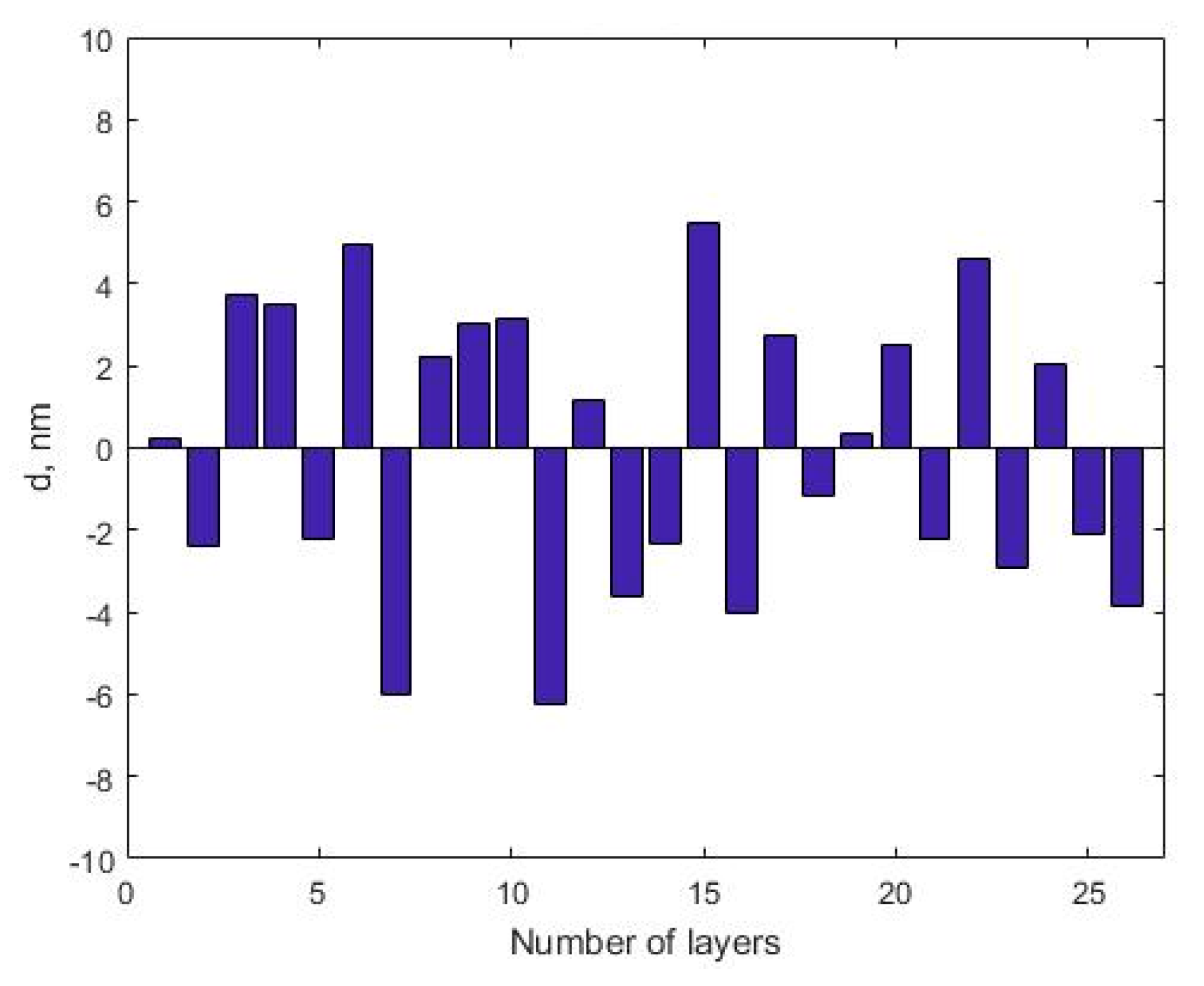
Figure 1 presents actual thickness errors da−dt in the case of one of the simulated deposition processes. Further results related to the online algorithms are presented for this particular case.
Twenty-six sets of simulated transmittance data corresponding to the end of deposition of the mirror layers are used as input data for the investigated characterization algorithms. Layer thicknesses that should be included in the list of unknown parameters in the case of modified S- and T-algorithms were found in accordance with Equation (6), where c is taken to be equal to 1 for both algorithms. The indices of the unknown parameters at each algorithm step are indicated in Table 1.
It can be seen that indeed in the case of the modified T-algorithm the number of searched for layer thicknesses are noticeably lower than the total number of layers at each new step of the algorithm. The maximum number of unknown parameters was eight for the triangular discrepancy function used after the deposition of layer number 15.
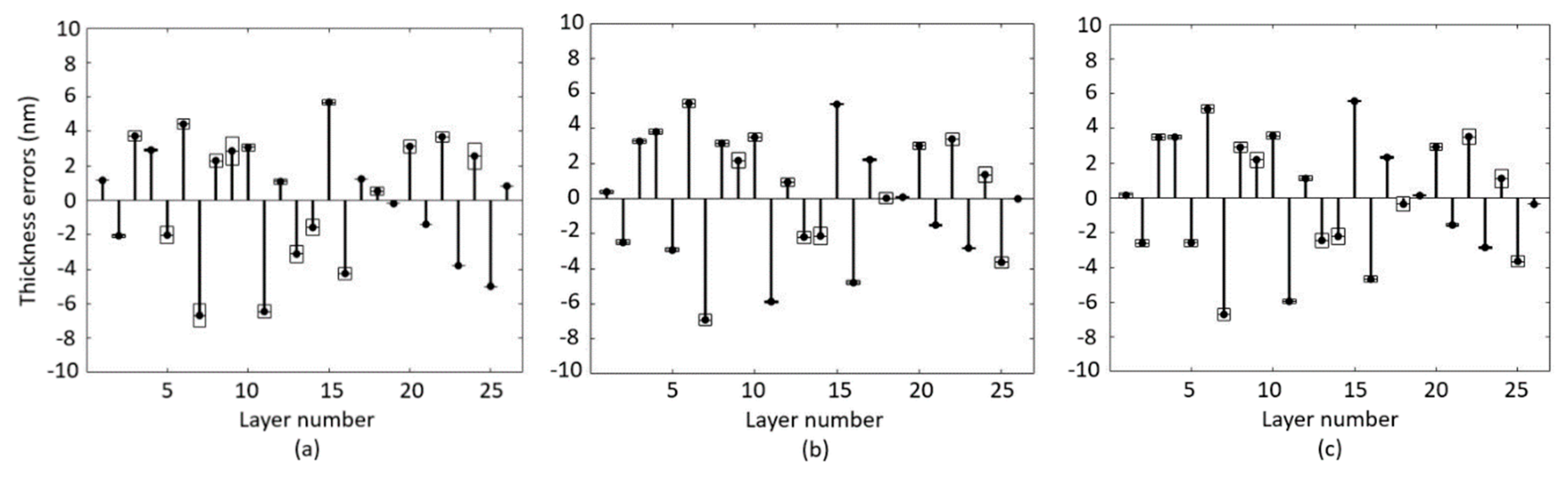
Figure 2 presents the errors in layer thicknesses found by all three algorithms. All layer thicknesses except for that of the last layer were determined at least two times. For this reason, Figure 2 shows the average values of the found thickness errors and also the corridor of fluctuation of these errors.
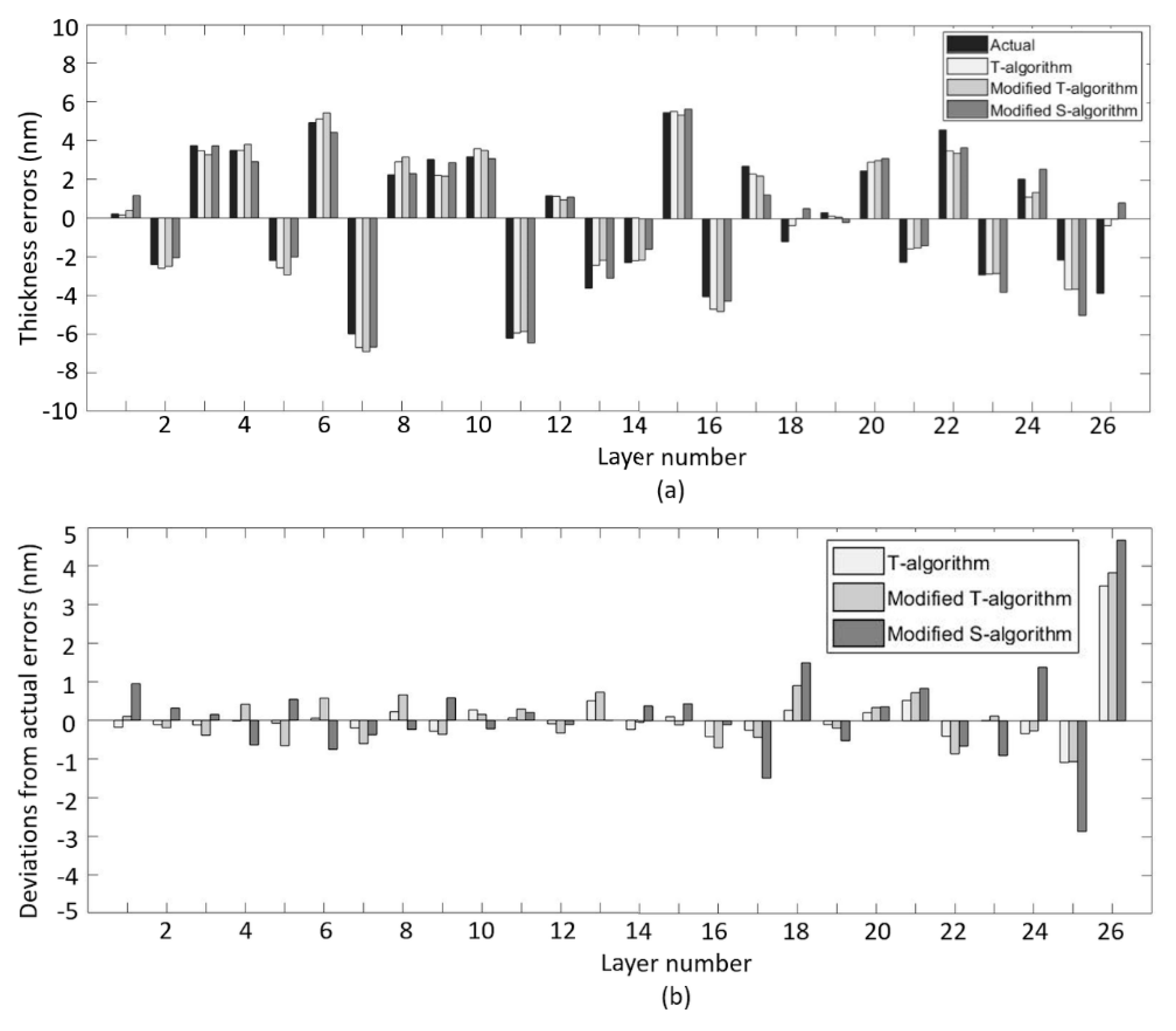
Figure 3 compares the average values of the found thickness errors with the actually-made thickness errors shown in Figure 1.
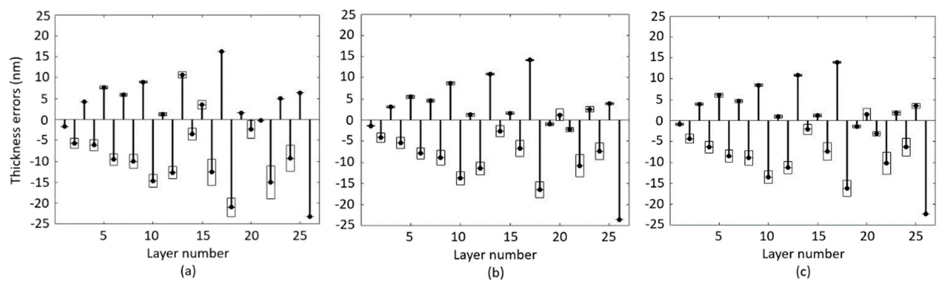
In the case of the real deposition runs we do not have information about the actual errors in layer thicknesses and we are not able to compare these errors with the errors determined by the investigated algorithms, as this is shown in Figure 3. Nevertheless, the comparison of the results obtained by all three algorithms can provide an indirect indication of their accuracy. This is shown in Figure 4 and Figure 5.
An important characteristic of an algorithm is its operational speed. For the considered 26-layer coating the relation between the operating time of the modified S-, modified T-, and T-algorithms was 1:17:128. Of course, this relation will be different for other coatings. However, the modified S-algorithm is always the fastest, while the T-algorithm is the most time-consuming. A discussion of all the above results is provided in the next section.
4. Discussion
The results presented in Figure 3 show that the thickness errors found by the investigated algorithms are close to the actual errors for almost all layers. In Figure 3a, the average values of the thickness errors found by all three algorithms are compared to the actual thickness errors known to the simulation software. To better estimate the accuracy of the algorithms, Figure 3b presents the differences between these values and actual errors. It is clearly seen that for almost all layers the best accuracy is provided by the T-algorithm. We performed analogous experiments with other sets of simulated transmittance data corresponding to several dozens of simulated deposition runs. It is worth noting that the indices of the determined layer thicknesses for the modified S- and T-algorithms were always the same, as indicated in Table 1. This was the case because the criterion for determining these indices depends only on the coating theoretical design. The results of the experiments performed were qualitatively the same as those presented in Figure 3.
In Figure 3, the largest differences between the found values and actual errors are observed for the last layer of the investigated coating. This is not surprising because the last layer is a low index layer with 2L optical thickness. In general, the accuracy of thickness determination is lower for all layer subsystems with L outer layers [20]. Additionally, with the nominal layer optical thickness equal to 2L, deviations of actual layer thickness from this nominal value have a very small effect on the coating spectral characteristics. It may be worth mentioning that the choice of double quarter-wave optical thickness for the last layer is usually based on considerations connected with improving laser damage resistance and thickness errors in this layer are not so dangerous. Finally, an accurate online characterization of the last layer is not important from the point of view of deposition process monitoring because its actual thickness is not required for the monitoring procedure.
The stability of layer thickness determination at different steps of a characterization algorithm is estimated by the level of fluctuation of the found thickness errors from their average value. If fluctuation is high, then accuracy of the thickness determination at some steps of the deposition process can be low and this can negatively influence the operation of the monitoring algorithm that is used to predict the termination instants of the layer deposition. In the case of the T- and modified T-algorithms these fluctuations are nearly the same, while in the case of the modified S-algorithm they are noticeably higher. This is observed both in the experiments with simulated and experimental measurement data (Figure 2 and Figure 4). Thus, we can say that from the point of view of accuracy, the T-algorithm is preferable to the modified S-algorithm.
Comparison of the T- and modified T-algorithms shows that they provide close characterization results: the found layer thickness errors are nearly the same in Figure 3 and Figure 5. The fluctuation of the found thickness errors are also close for these algorithms. Thus we can conclude that these algorithms are close in accuracy. At the same time, the modified T-algorithm is considerably faster. This advantage is perhaps not very significant when the number of coating layers is in the range of two–three dozen. However, it becomes more and more important with the growing number of coating layers. It is not rare that broadband monitoring is used for the production of coatings with many dozens of layers and the operational speed of the modified T-algorithm may prove to be the decisive factor when choosing it as the main online characterization algorithm in modern broadband monitoring systems.
Simulation experiments to compare modified S-, modified T-, and T-algorithms were also carried out using other non-quarter-wave designs such as hot mirror and Brewster angle polarizer. Of course, for other designs the tables of indices of determined layer thicknesses were different from Table 1. However, the number of parameters determined by Modified T-algorithm was always noticeably smaller than the total number of layers at the respective algorithm steps. This provides better performance for this algorithm compared to the T-algorithm. At the same time, the accuracy of these algorithms is comparable. As a further prospect for increasing the speed of the modified T-algorithm, one can try to reduce the number of partial discrepancy functions in Equation (3) by removing some of the least informative measurement data. This question requires, however, a deeper theoretical analysis in the future.
Author Contributions
Conceptualization, A.T.; Methodology, A.T.; Software, T.I. and D.L.; Validation, I.K. and D.L.; Formal Analysis, A.T., I.K. and A.Y.; Investigation, A.T. and T.I.; Writing-Original Draft Preparation, A.T.; Writing-Review and Editing, A.T. and I.K.; Funding Acquisition, A.T. and A.Y.; Supervision, A.T. and A.Y.
Funding
This research was funded by Russian Scientific Foundation grant No. 16-11-10219.
Conflicts of Interest
The authors declare no conflict of interest.
References
- Macleod, H.A. Monitoring of optical coatings. Appl. Opt. 1981, 20, 82–89. [Google Scholar] [CrossRef] [PubMed]
- Macleod, H.A. Thin-Film Optical Filters, 4th ed.; CRC Press, Taylor & Francis Group: Boca Raton, FL, USA, 2010. [Google Scholar]
- Ehlers, H.; Ristau, D. Production strategies for high precision optical coatings. In Optical Thin Films and Coatings; Piegari, A., Flory, F., Eds.; Woodhead: Cambridge, UK, 2013; pp. 94–130. [Google Scholar]
- Tikhonravov, A.; Trubetskov, M.; Amotchkina, T. Optical monitoring strategies for optical coating manufacturing. In Optical Thin Films and Coatings, 2nd ed.; Piegari, A., Flory, F., Eds.; Woodhead: Cambridge, UK, 2018; pp. 65–101. [Google Scholar]
- Starke, K.; Gross, T.; Lappschies, M.; Ristau, D. Rapid prototyping of optical thin film filters. Proc. SPIE 2000, 4094, 83–92. [Google Scholar]
- Hofman, D.; Sassolas, B.; Michel, C.; Balzarini, L.; Pinard, L.; Teillon, J.; David, B.; Lagrange, B.; Barthelemy-Mazot, E.; Gagnoli, G. Photometric calibration of an in situ broadband optical thickness monitoring of thin films in a large vacuum chamber. Appl. Opt. 2017, 56, 409–416. [Google Scholar] [CrossRef] [PubMed]
- Lappschies, M.; Gross, T.; Ehlers, H.; Ristau, D. Broadband optical monitoring for the deposition of complex coatings. Proc. SPIE 2004, 5250, 637–645. [Google Scholar] [CrossRef]
- Ristau, D.; Ehlers, H.; Gross, T.; Lappschies, M. Optical broadband monitoring of conventional and ion processes. Appl. Opt. 2006, 45, 1495–1501. [Google Scholar] [CrossRef] [PubMed]
- Friedrich, K.; Wilbrandt, S.; Stenzel, O.; Kaiser, N.; Hoffmann, K.H. Computational manufacturing of optical interference coatings: Method, simulation results, and comparison with experiment. Appl. Opt. 2010, 49, 3150–3162. [Google Scholar] [CrossRef] [PubMed]
- Vidal, B.; Fornier, A.; Pelletier, E. Optical monitoring of nonquarterwave multilayer filters. Appl. Opt. 1978, 17, 1038–1047. [Google Scholar] [CrossRef] [PubMed]
- Zhupanov, V.; Kozlov, I.; Fedoseev, V.; Konotopov, P.; Trubetskov, M.; Tikhonravov, A. Production of Brewster-angle thin film polarizers using ZrO2/SiO2 pair of materials. Appl. Opt. 2017, 56, C30–C34. [Google Scholar] [CrossRef] [PubMed]
- Tikhonravov, A.; Trubetskov, M.; Amotchkina, T. Investigation of the effect of accumulation of thickness errors in optical coating production using broadband optical monitoring. Appl. Opt. 2006, 45, 7026–7034. [Google Scholar] [CrossRef] [PubMed]
- Zöller, A.; Williams, J.; Hartlaub, S. Precision filter manufacture using direct optical monitoring. In Proceedings of the Optical Interference Coatings, Tucson, AZ, USA, 6–11 June 2010. Paper TuC8. [Google Scholar] [CrossRef]
- Zöller, A.; Hagedorn, H.; Weinrich, W.; Wirth, E. Testglass changer for direct optical monitoring. Proc. SPIE 2011, 8168, 81681J. [Google Scholar] [CrossRef]
- Zöller, A.; Arhilger, D.; Boos, M.; Hagedorn, H. Advanced optical monitoring system using a newly developed low noise wideband spectrometer system. Proc. SPIE 2015, 9627, 9627–9638. [Google Scholar] [CrossRef]
- Zöller, A.; Arhilger, D.; Boos, M.; Hagedorn, H.; Reus, H. High throughput PIAD with an advanced RF-plasma source and direct optical monitoring. In Proceedings of the Optical Interference Coatings (OIC), Tucson, AZ, USA, 19–24 June 2016. [Google Scholar] [CrossRef]
- Ristau, D.; Ehlers, H.; Schlichting, S.; Lappschies, M. State of the art in deterministic production of optical thin films. Proc. SPIE 2008, 7101, 71010C. [Google Scholar] [CrossRef]
- Stenzel, O.; Wilbrandt, S.; Kaiser, N.; Fasold, D. Development of a hybrid monitoring strategy to the deposition of chirped mirrors by plasma-ion assisted electron evaporation. Proc. SPIE 2008, 7101, 71011Y. [Google Scholar] [CrossRef]
- Ehlers, H.; Schlichting, S.; Schmitz, C.; Ristau, D. From independent thickness monitoring to adaptive manufacturing: Advanced deposition control of complex optical coatings. Proc. SPIE 2011, 8168, 81681F. [Google Scholar] [CrossRef]
- Tikhonravov, A.V.; Trubetskov, M.K. Online characterization and re-optimization of optical coatings. Proc. SPIE 2004, 5250, 406–413. [Google Scholar]
- Wilbrandt, S.; Stenzel, O.; Kaiser, N.; Trubetskov, M.K.; Tikhonravov, A.V. In situ optical characterization and reengineering of interference coatings. Appl. Opt. 2008, 47, C49–C54. [Google Scholar] [CrossRef] [PubMed]
- Amotchkina, T.V.; Trubetskov, M.K.; Pervak, V.; Schlichting, S.; Ehlers, H.; Ristau, D.; Tikhonravov, A.V. Comparison of algorithms used for optical characterization of multilayer optical coatings. Appl. Opt. 2011, 50, 3389–3395. [Google Scholar] [CrossRef] [PubMed]
- Tikhonravov, A.V.; Gorokh, A. Modified sequential algorithm for the online characterization of optical coatings. Opt. Express 2015, 23, 23561–23569. [Google Scholar] [CrossRef] [PubMed]
- Isaev, T.F.; Kochikov, I.V.; Lukyanenko, D.V.; Tikhonravov, A.V.; Yagola, A.G. Improving the accuracy of broad-band monitoring of optical coating deposition. Mosc. Univ. Phys. Bull. 2018, 73, 382–387. [Google Scholar] [CrossRef]
Figure 1.
Deviations of actual layer thickness from the theoretically planned layer thickness in one of the simulated deposition processes.
Figure 1.
Deviations of actual layer thickness from the theoretically planned layer thickness in one of the simulated deposition processes.

Figure 2.
Average values of thickness errors and fluctuations of thickness errors found by the modified S-algorithm (a); modified T-algorithm (b); and T-algorithm (c).
Figure 2.
Average values of thickness errors and fluctuations of thickness errors found by the modified S-algorithm (a); modified T-algorithm (b); and T-algorithm (c).

Figure 3.
Comparison of the average values of thickness errors found by all three algorithms with actually made thickness errors (a) and differences between these values and actual errors (b).
Figure 3.
Comparison of the average values of thickness errors found by all three algorithms with actually made thickness errors (a) and differences between these values and actual errors (b).

Figure 4.
Results of the characterization using online transmittance data from the real deposition run: average values of thickness errors and fluctuations of thickness errors found using the modified S-algorithm (a); modified T-algorithm (b); and T-algorithm (c).
Figure 4.
Results of the characterization using online transmittance data from the real deposition run: average values of thickness errors and fluctuations of thickness errors found using the modified S-algorithm (a); modified T-algorithm (b); and T-algorithm (c).

Figure 5.
Results of the characterization using online transmittance data from the real deposition run: comparison between average values of thickness errors found by the investigated algorithms.
Figure 5.
Results of the characterization using online transmittance data from the real deposition run: comparison between average values of thickness errors found by the investigated algorithms.


Table 1.
Indices of the determined layer thicknesses for the modified S- and T-algorithms.
| Algorithm Step | Indices of Determined Layer Thicknesses | |
|---|---|---|
| Modified S-Algorithm (c = 1) | Modified T-Algorithm (c = 1) | |
| 1 | 1 | 1 |
| 2 | 2 | 1, 2 |
| 3 | 2, 3 | 1, 2, 3 |
| 4 | 4 | 1, 2, 3, 4 |
| 5 | 3, 4, 5 | 1, 2, 3, 4, 5 |
| 6 | 6 | 1, 2, 3, 4, 5, 6 |
| 7 | 4, 5, 6, 7 | 4, 5, 6, 7 |
| 8 | 4, 8 | 4, 5, 6, 7, 8 |
| 9 | 5, 6, 7, 8, 9 | 5, 6, 7, 8, 9 |
| 10 | 5, 10 | 5, 7, 8, 9, 10 |
| 11 | 6, 7, 8, 9, 10, 11 | 6, 7, 8, 9, 10, 11 |
| 12 | 6, 12 | 6, 9, 10, 11, 12 |
| 13 | 7, 8, 9, 10, 12, 13 | 7, 8, 9, 10, 11, 12, 13 |
| 14 | 7, 14 | 7, 11, 12, 13, 14 |
| 15 | 8, 9, 10, 11, 12, 13, 14, 15 | 8, 9, 10, 11, 12, 13, 14, 15 |
| 16 | 8, 16 | 8, 12, 13, 14, 15, 16 |
| 17 | 9, 10, 11, 12, 16, 17 | 9, 10, 11, 12, 15, 16, 17 |
| 18 | 9, 14, 18 | 9, 10, 14, 15, 16, 17, 18 |
| 19 | 10, 11, 12, 13, 14, 18, 19 | 10, 11, 12, 17, 18, 19 |
| 20 | 10, 20 | 10, 11, 17, 18, 19, 20 |
| 21 | 11, 12, 13, 14, 20, 21 | 11, 12, 14, 19, 20, 21 |
| 22 | 11, 18, 22 | 11, 12, 19, 20, 21, 22 |
| 23 | 12, 13, 14, 15, 16, 22, 23 | 12, 13, 14, 22, 23 |
| 24 | 12, 24 | 12, 13, 14, 21, 22, 23, 24 |
| 25 | 13, 14, 15, 16, 24, 25 | 13, 14, 24, 25 |
| 26 | 14, 15, 16, 26 | 13, 14, 24, 25, 26 |
© 2018 by the authors. Licensee MDPI, Basel, Switzerland. This article is an open access article distributed under the terms and conditions of the Creative Commons Attribution (CC BY) license (http://creativecommons.org/licenses/by/4.0/).
Share and Cite
MDPI and ACS Style
Tikhonravov, A.; Kochikov, I.; Isaev, T.; Lukyanenko, D.; Yagola, A. Online Characterization Algorithms for Optical Coating Production with Broadband Monitoring. Coatings 2018, 8, 323. https://doi.org/10.3390/coatings8090323
AMA Style
Tikhonravov A, Kochikov I, Isaev T, Lukyanenko D, Yagola A. Online Characterization Algorithms for Optical Coating Production with Broadband Monitoring. Coatings. 2018; 8(9):323. https://doi.org/10.3390/coatings8090323
Chicago/Turabian StyleTikhonravov, Alexander, Igor Kochikov, Temur Isaev, Dmitry Lukyanenko, and Anatoly Yagola. 2018. "Online Characterization Algorithms for Optical Coating Production with Broadband Monitoring" Coatings 8, no. 9: 323. https://doi.org/10.3390/coatings8090323
Note that from the first issue of 2016, this journal uses article numbers instead of page numbers. See further details here.