1. Introduction
Surface plasmon resonance (SPR) spectroscopy exploits the excitation of surface plasmons to follow molecular interactions in real-time without the need for additional molecular labels. A ‘surface plasmon’ represents a surface charge density wave at a metal-dielectric interface [
1]. Light couples to the surface plasmon, and resonance occurs when its propagation constant equals the wave vector of light that is parallel to the interface [
1,
2,
3]. The majority of SPR systems are based on the Kretschmann configuration [
4,
5], in which incident light passes through a prism that has a high refractive index, and is totally reflected at the metal-prism interface [
2,
3]. This generates a penetrating evanescent field which decays exponentially into the dielectric if the metal interface (typically gold) is sufficiently thin (less than 100 nm for visible and near infrared light) [
2,
3,
6]. A binding-induced change in the dielectric refractive index leads to change in one or more light characteristics, such as the angle, phase, wavelength, or intensity. This latter change is needed to excite the surface plasmon wave [
3]. Most SPR biosensors use the angle of the reflected light to monitor binding events. To achieve this, a wedge-shaped beam of monochromatic light is directed onto the metal interface to cover numerous angles of incidence [
7]. The intensity of the reflected light reaches its minimum when the surface plasmon gets excited. The angle of incidence at which this dip occurs represents the sensor signal which is usually presented in a sensorgram as a function of time [
3].
Human serum albumin (HSA) is exclusively synthesized in the liver, and is the most abundant plasma protein (60%, 40 mg/mL) [
8,
9,
10]. The monomer is responsible for the preservation of pH and osmotic pressure, as well as for the transport of numerous substances such as metals, fatty acids, amino acids, hormones, vitamins and drugs [
9,
10,
11,
12]. HSA is a heart-shaped, 585 amino acids long protein (66.5 kDa) which consists of three homologue domains [
12,
13]. Due to its 17 disulfide bridges, this negatively-charged, single-chain protein has an average half-life of 19 days and remains stable at temperatures up to 60 °C as well as in pHs ranging from 7 to 9 [
12,
14].
About 20%–30% of the body’s hepatocytes are busy producing HSA at any given moment [
15]. Therefore, HSA concentrations in plasma can be used as a reliable marker for the diagnosis and prognosis of various diseases [
16]. For example, liver diseases are probable if the concentration of HSA in blood falls below the index value of 40 mg/mL [
16,
17]. HSA concentrations of approximately 20 mg/mL can indicate liver cirrhosis. Furthermore, HSA is one of the main nutrients for tumors. As a result, HSA levels in cancer patients may be low depending on the size and activity of their tumors [
12]. Additionally, HSA can be used to test the viability of human hepatocytes cultivated
in vitro [
18,
19,
20]. Such cultivated liver tissues are of great interest in pharmacologic research because of their potential for predictive substance evaluation [
20,
21].
In this study, we used the
liSPR system to investigate the binding mechanism and determine the affinity of the HSA-antibody interaction involved. Affinity is normally represented as a dissociation constant,
KD, which displays the concentration of an analyte at which half of the free ligand will be bound within a complex at equilibrium [
22]. Thus, high
KD values signify low affinities. The affinities of antibody-antigen reactions typically appear in the micromolar to picomolar range [
23].
The simplest model involves 1:1 binding. This model is based on the assumption that one analyte (A) molecule will bind to one ligand (L) molecule (A + L ↔ LA) [
24]. However, we used polyclonal antibodies, which are a mixture of antibodies with different specificities and affinities for their antigen [
25]. Thus, a more complex model is a better choice for imitating real binding. The heterogeneous analyte model, for example, assumes that two independent analytes will compete to bind to one ligand (A1 + L ↔ LA1, A2 + L ↔ LA2). Hence, two affinity constants will be determined. In contrast, the bivalent analyte model describes the interaction between a bivalent analyte to one or two ligands. In the first step of the binding reaction (A + L ↔ LA), the two ligand binding sites remain equivalent, and in the second step (LA + L ↔ LLA), cooperative effects contribute [
24]. The second binding step depends on the flexibility of the monovalent bound ligand-analyte complex (LA) as well as its proximity to the next ligand molecule [
26], and leads to stabilization of the resulting complex. The second association rate of the bivalent analyte model is reported in the unit Pixel
−1s
−1 instead of M
−1s
−1, because the local concentration of the analyte is taken into account.
In the proposed sensor, HSA was covalently attached to the carboxylated self-assembled monolayer (SAM) via its lysine residues by amine coupling procedure. The interactions of high-affinity antibodies with the immobilized HSA were investigated using the low-cost bench-top
liSPR system [
7]. A lack of appropriate software for evaluating the computation of binding constants by the
liSPR system led to the implementation and evaluation of different algorithms for modeling the types of binding. To the best of our knowledge, this was the first time that kinetics studies of a HSA-antibody interaction were performed using SPR.
3. Results and Discussion
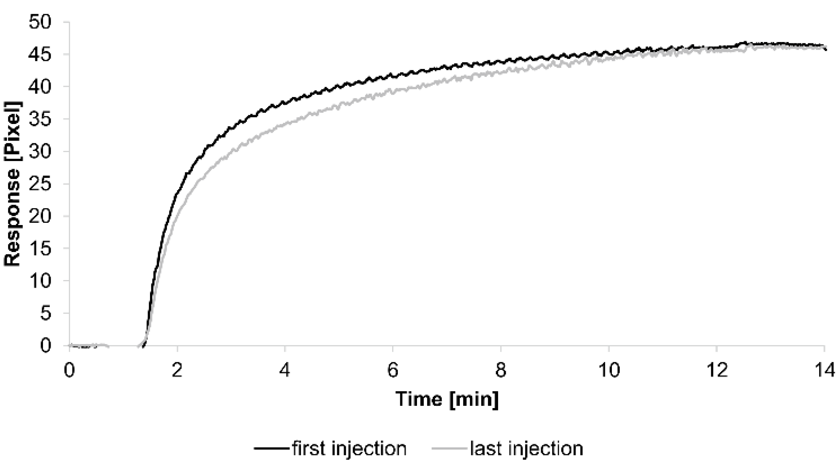
For the kinetic analyses, HSA was attached to a sensor chip by the amine coupling procedure. To show the reproducibility of our assay we injected 0.7 µM HSA-specific antibody immediately before and after the kinetic measurements (see below) (
Figure 1).
The curves obtained from both injections were quite similar, demonstrating the reliability of the assay. Additionally, each tested concentration was analyzed using two sensing and two reference spots.
For kinetic measurements, antibody solutions ranging in concentration from 3.4 nM to 3.4 µM were sequentially injected. Data representing binding of the antibodies to HSA were evaluated using three different models.
Figure 2,
Figure 3 and
Figure 4 show overlaid fits of different binding models, and the parameters are presented in
Table 1.
Figure 1.
Sensorgrams showing the binding response of injections of 0.7 µM human serum albumin (HSA)-specific antibody before and after the kinetic measurements. Values resulting from the average of two sensing spots and the subtraction of reference surface signals from raw signal measurements are presented on the graph.
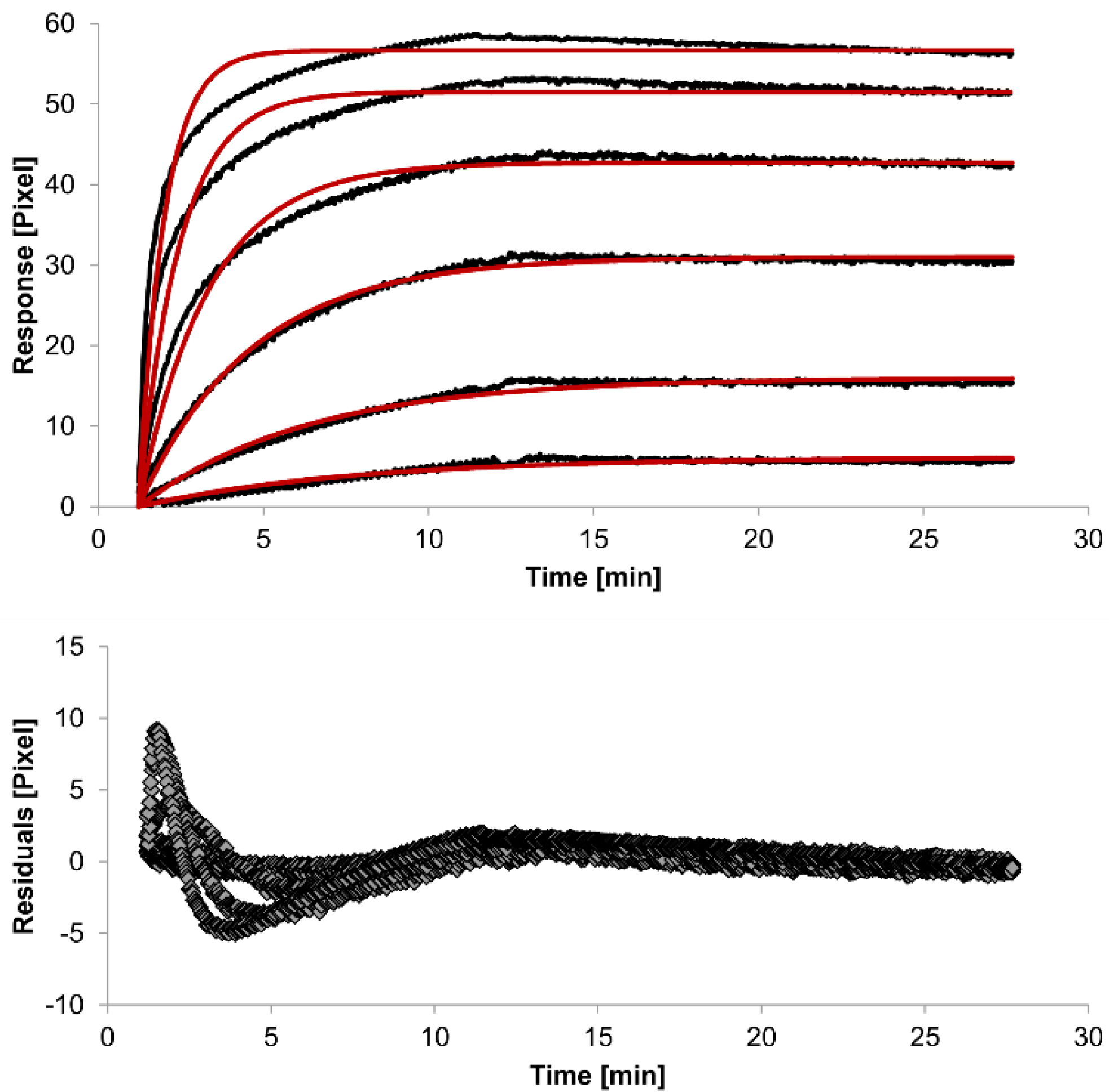
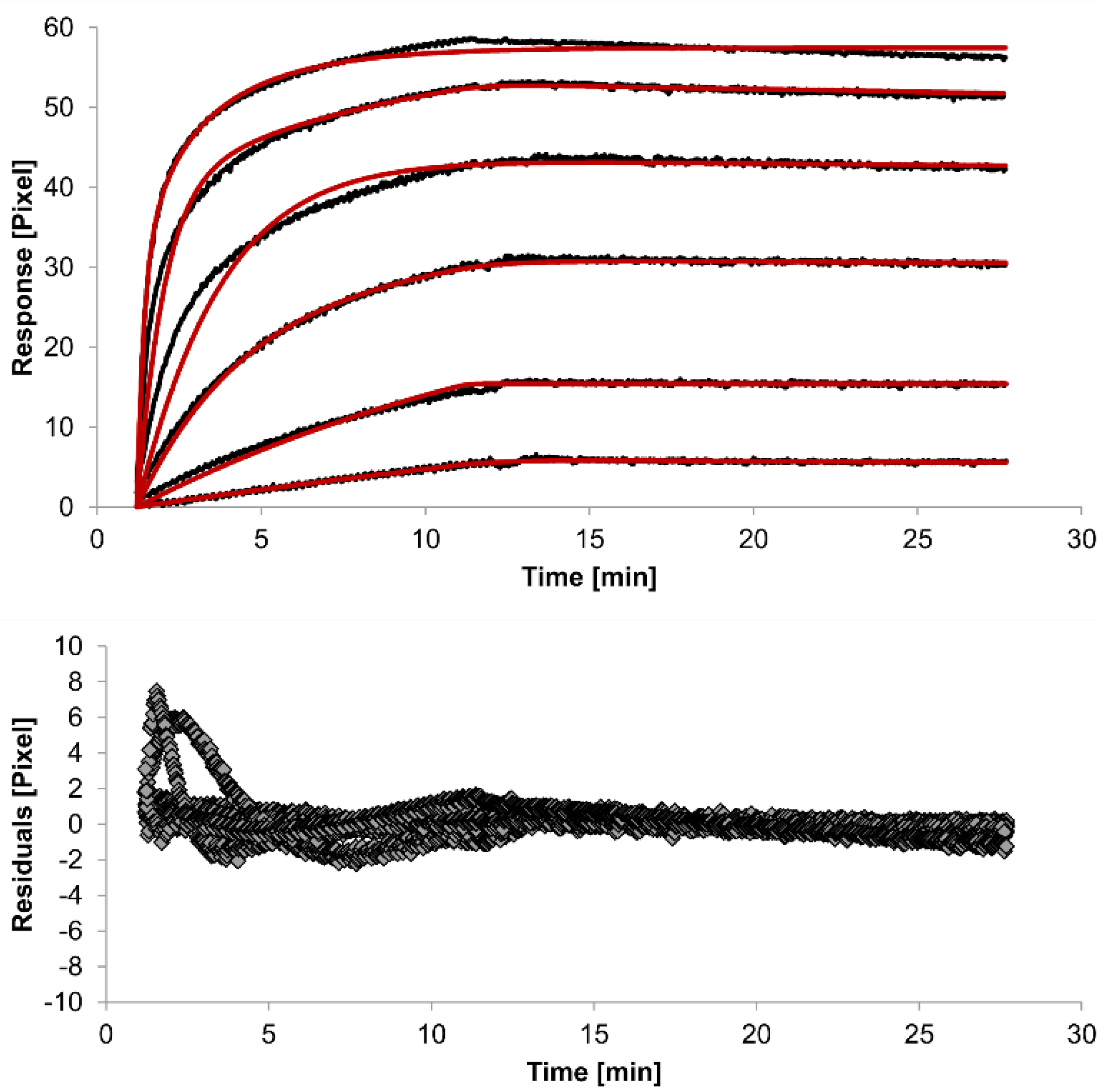
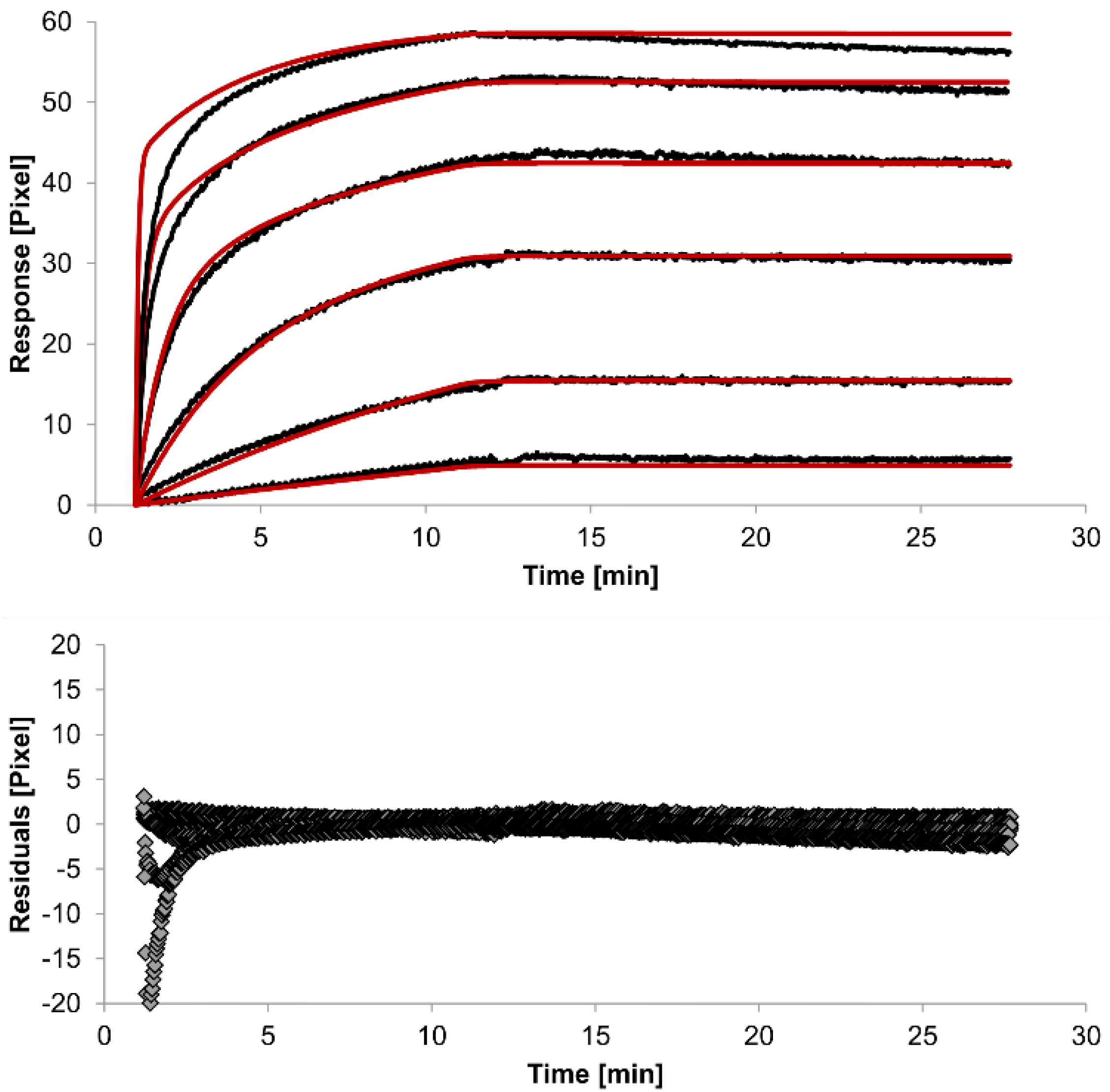
A decision as to whether the fit is acceptable can be made based on visual inspection of the overlaid fit and the residuals. The residuals are the deviation between the experimental data and the modelled binding curve and provide an indication if the choice of the binding model is appropriate. The residuals should be roughly normally and independently distributed with zero mean.
The overlays and residuals of the 1:1 binding (
Figure 2), heterogeneous analyte (
Figure 3) and bivalent analyte (
Figure 4) models, from local fitting of rate constants, show different results for goodness of fit. The main deviation between the models and the experimental data appeared during the association phase. Visual inspections of the results indicate that the experimental data were best fitted to the heterogeneous analyte binding model. Good results were also obtained with the bivalent analyte model whereas, the 1:1 binding model produced the worst fit.
Another way to measure goodness of fit is the Chi-squared (χ
2) value, which reflects the differences between measured and expected (modelled) values (the smaller the value, the better the fit). Since the χ
2 value depends on signal intensity, the values for the different immobilization levels should not be compared to each other. Nevertheless, the values of the χ
2 are shown in
Table 1.
Table 1.
Kinetic parameters obtained from local fitting of the interaction between the immobilized HSA and HSA-specific antibody for each mathematical model. The average rate constant and standard error of the local fit values for each model are reported.
Table 1.
Kinetic parameters obtained from local fitting of the interaction between the immobilized HSA and HSA-specific antibody for each mathematical model. The average rate constant and standard error of the local fit values for each model are reported.
| Interaction Model | ka1
[M−1s−1] | kd1
[s−1] | ka2
[M−1s−1] | kd2
[s−1] | χ2
[Pixel2] |
|---|
| 1:1 binding | 4 (± 1)
×104 | 2.1 (± 0.2)
×10−3 | / | / | 1.8 |
| heterogeneous analyte | 2.3 (± 0.9)
×104 | 1.2 (± 0.4)
×10−2 | 5 (± 2)
×104 | 7 (± 4)
×10−4 | 0.1 |
| bivalent analyte | 3.1 (± 0.7)
×104 | 1.8 (± 0.7)
×10−4 | 1.2 (± 0.7)
×106
[Pixel−1s−1] | 9 (± 5)
×10−3 | 0.8 |
Figure 2.
Kinetics of HSA-specific antibodies binding to immobilized HSA. Plots generated by applying the 1:1 binding model (red lines) overlay the plots associated with each antibody concentration (black lines; from top to bottom: 3.4 µM, 0.9 µM, 0.2 µM, 53.9 nM, 13.5 nM, 3.4 nM). Values resulting from the average of two sensing spots and the subtraction of reference surface signals from raw signal measurements are presented on the graph. The graph below depicts the residuals of the fits.
Figure 3.
Kinetics of HSA-specific antibodies binding to immobilized HSA. Plots generated by applying the heterogeneous analyte model (red lines) overlay the plots associated with each antibody concentration (black lines; from top to bottom: 3.4 µM, 0.9 µM, 0.2 µM, 53.9 nM, 13.5 nM, 3.4 nM). Values resulting from the average of two sensing spots and the subtraction of reference surface signals from raw signal measurements are presented on the graph. The graph below depicts the residuals of the fits.
Figure 4.
Kinetics of HSA-specific antibodies binding to immobilized HSA. Plots generated by applying the bivalent analyte model (red lines) overlay the plots associated with each antibody concentration (black lines; from top to bottom: 3.4 µM, 0.9 µM, 0.2 µM, 53.9 nM, 13.5 nM, 3.4 nM). Values resulting from the average of two sensing spots and the subtraction of reference surface signals from raw signal measurements are presented on the graph. The graph below depicts the residuals of the fits.
The 1:1 binding model shows the highest χ
2 value (1.8). This is not surprising because 1:1 binding is biologically implausible when an antibody is the analyte. In contrast, the heterogeneous analyte model best agrees with the experimental data. However, this model assumes that the analyte consists of two different HSA-specific species only, which might not be true for polyclonal antibodies. The χ
2-value of the bivalent analyte model is 0.8, which lies between the values for the 1:1 binding and heterogeneous analyte models and represents a good data fit. Since antibodies are bivalent molecules, this model is most probable biologically. The resulting rate constants for the three models are summarized in
Table 1. The average rate constant and the standard error with respect to the local fit (specific for every binding curve) are reported for each binding curve.
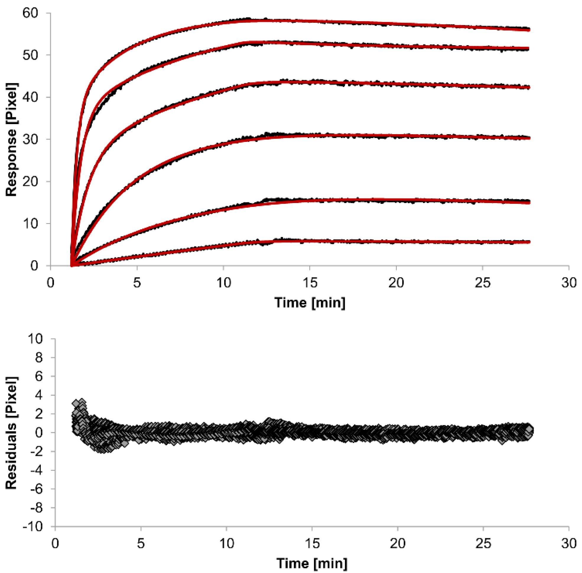
In spite of the above, the rate constants should be globally applied to all concentrations to achieve reliable results. Thus, global fitting of the rate constants was performed. Rate constants were calculated for the whole data set. Only the bivalent analyte model produced an acceptable global fit (
Figure 5).
We observed an affinity (
KD) of 37 pM (k
a1 = 4.261 (±0.002) × 10
4 M
−1s
−1, k
d1 = 1.58 (±0.06) × 10
−6 s
−1) for the first (monovalent) binding step, with a χ
2 value of 1.4 Pixels
2. These values show that the global parameters fit the experimental data less accurately than the locally determined parameters. The affinity for the second (bivalent) binding step was measured at 20 pM (
ka2 = 4.900 (±0.002) × 10
5 RU
−1s
−1,
kd2 = 8.420 (±0.007) × 10
−3s
−1). In fact, the dissociation rate for the bivalent binding step was much faster than for the monovalent binding step. This might be expected because monovalent binding occurs with free analytes whereas bivalent binding occurs with monovalently bound analytes [
26]. The standard error of the globally determined parameters reflects the degree of uncertainty of the rate constants and are a measure for reliability. Considering all these factors, the bivalent analyte model seems to best represent the interaction between HSA and the antibody.
Figure 5.
Kinetics of HSA-specific antibodies binding to immobilized HSA. Plots generated by globally applying the bivalent analyte model (red lines) overlay the plots associated with each antibody concentration (black lines; from top to bottom: 3.4 µM, 0.9 µM, 0.2 µM, 53.9 nM, 13.5 nM, 3.4 nM). Values resulting from the average of two sensing spots and the subtraction of reference surface signals from raw signal measurements are presented on the graph. The graph below depicts the residuals of the fits.


