3.1. Dielectrophoresis
During the dielectrophoresis process, the AC source applied across the electrodes generates a non-uniform electric field, which causes the electrons and protons in the SWNTs to move away from their balanced positions. The redistribution of the charges creates electric dipoles in the SWNTs. The interactive force between the dipoles and the non-uniform electric field is called dielectrophoretic force
F, which is expressed as [
26,
27]:
where the term
πr2l/6 is a geometry factor that contains the volume information of the nanotube,
em is the permittivity of the solvent medium,
Re[
fcm] is the real number part of the Clausius-Mossotti factor
fcm, and
▽Erms is the gradient of the root mean square of the external electric field. As a result of the dielectrophoretic force, the SWNTs are able to move and rotate in the solution to follow the directions of the electric field lines.
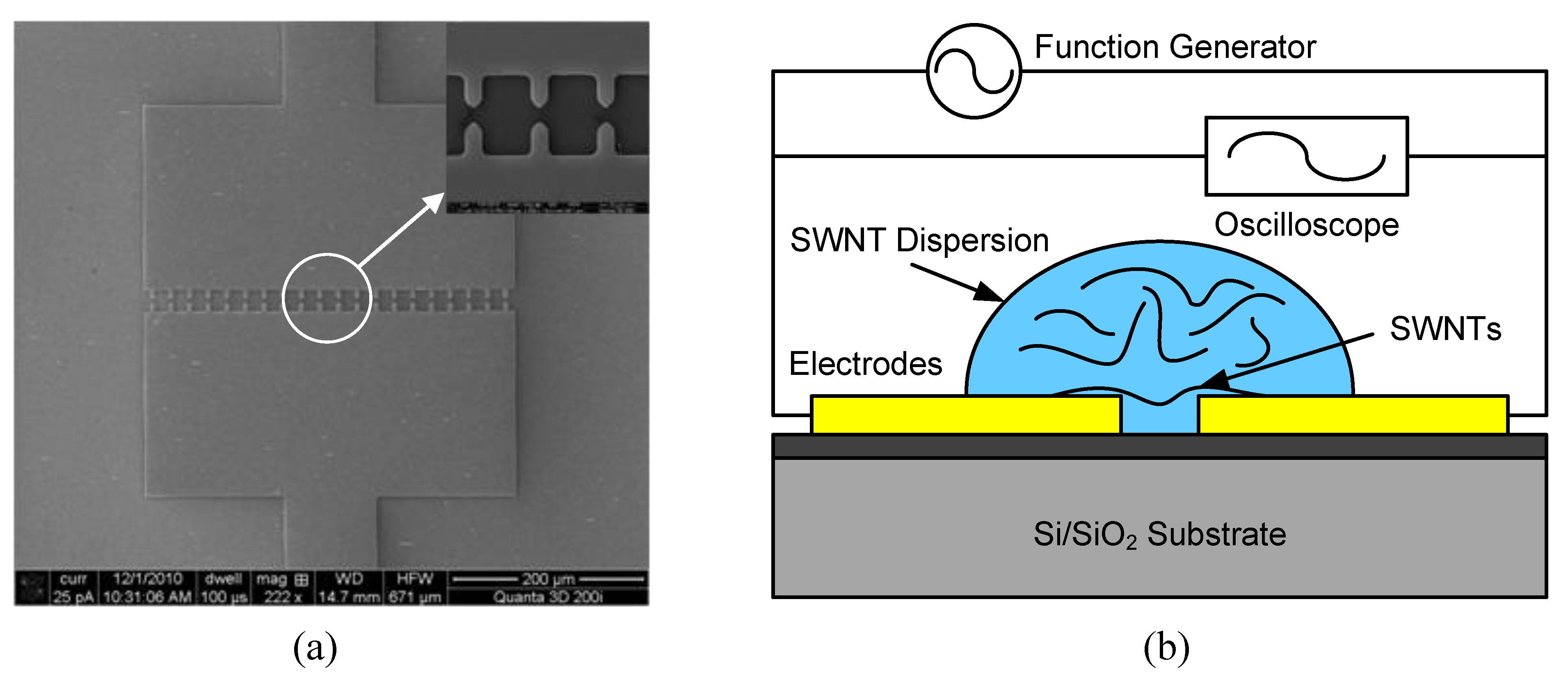
To align the SWNTs, a small drop of the SWNT solution is placed on the substrate to cover the electrodes using a syringe. Next, the function generator is switched on; an AC electric field is generated between the electrodes. The electric field exerts dielectrophoretic forces on the SWNTs and forces them to rotate along the field lines. As a result, the SWNTs are rapidly attracted by the dielectrophoretic force and landed on the substrate across the electrodes. An instant voltage drop of 1–2 V can be observed from the oscilloscope during the capturing event. The typical time range of the dielectrophoresis process in our investigation is 30 s. Next, the solution residual is removed with a syringe. The dielectrophoretically assembled SWNTs are inspected with an SEM, as shown in
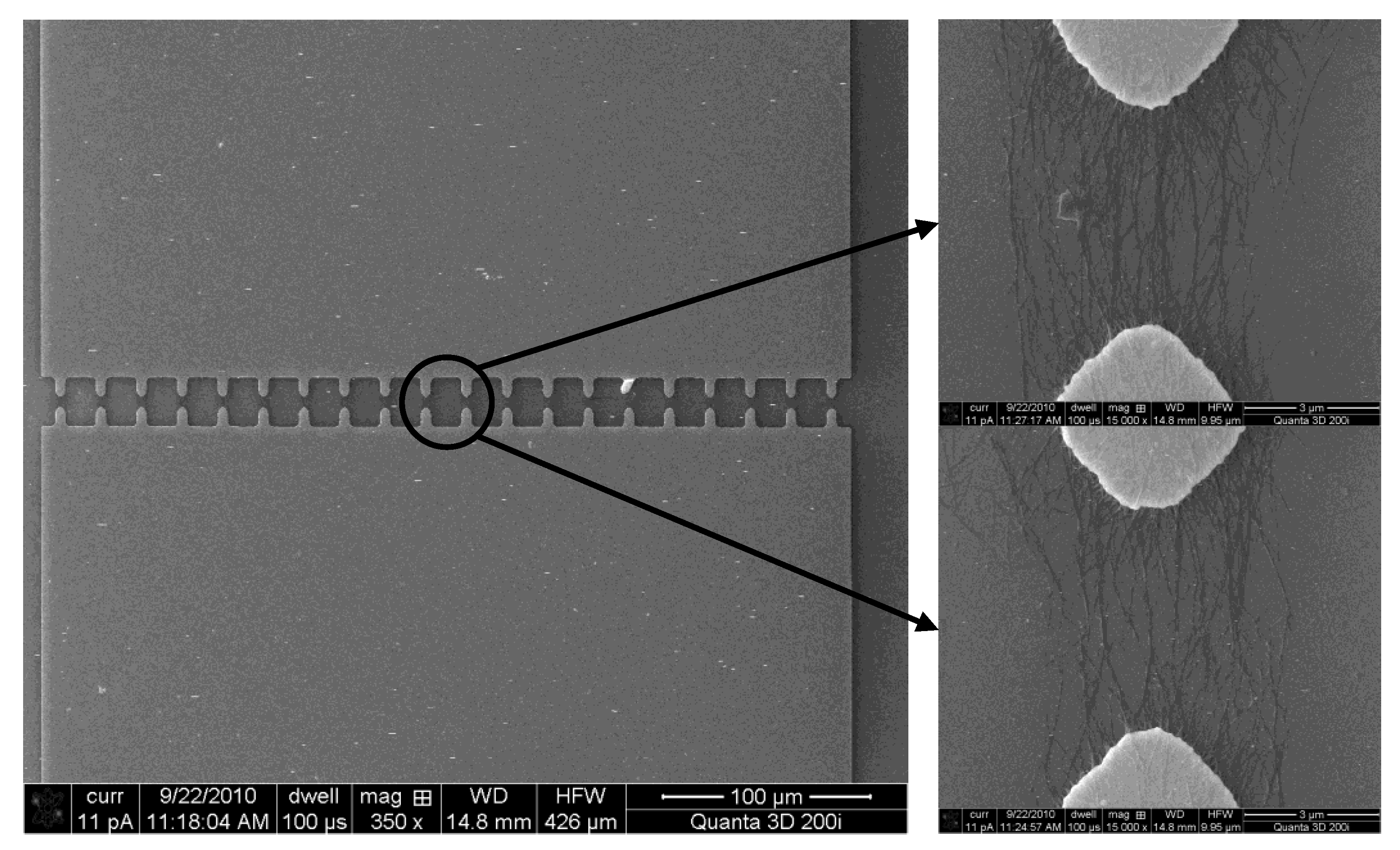
Figure 4. Although the exact number of aligned SWNTs varies from one electrode pair to another, the alignment results and the amount of aligned SWNTs are relatively consistent. The SWNTs are mainly in the form of bundles and they can only be observed in between the electrode pairs, where the electric field has the highest magnitude.
Figure 4.
SEM images of the sensor structure and the dielectrophoretically aligned SWNTs.
Figure 4.
SEM images of the sensor structure and the dielectrophoretically aligned SWNTs.
3.2. pH Sensitivity
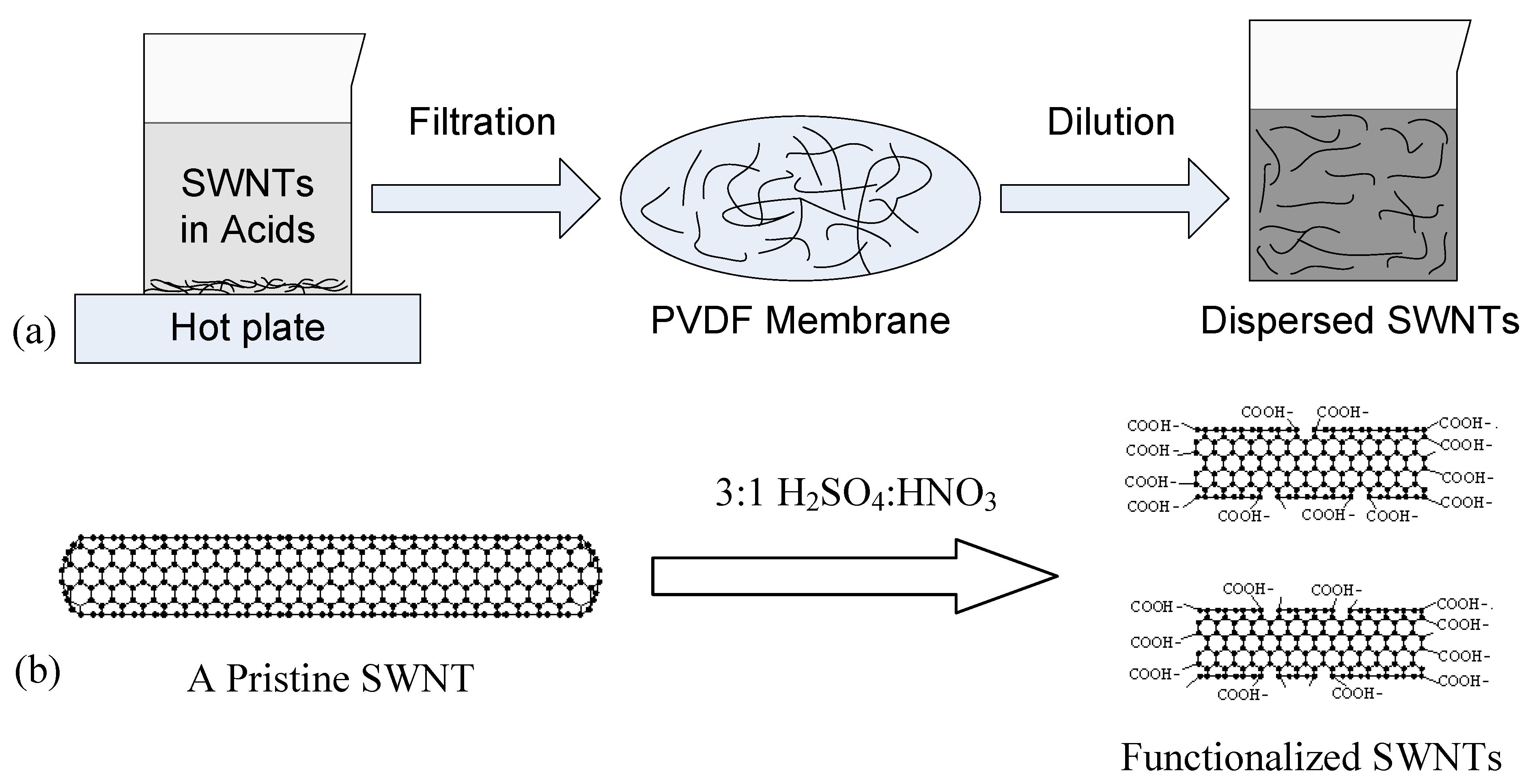
Early study showed that the pristine SWNT is a p-type material,
i.e., the majority charge carriers are holes. The acid-functionalized SWNTs also demonstrated p-type characteristics when used in electronic devices [
28]. When such SWNTs are submerged in pH buffer solutions, hydrogen (H
+) and hydroxide (OH
−) ions can interact with the carboxyl groups covalently attached to the SWNTs. Hydrogen (H
+) as a proton is able to bind to the surface of the SWNT and accept one electron from the p-orbital of the nanotube. This induces the generation of a positive hole in the SWNT and increases its conductance [
11]. At the same time, the hydroxide (OH
−) ions cause the opposite effects, decreasing the conductance of the SWNT. Consequently, the concentrations of H
+ and OH
− ions affect the generation of holes and electrons in the SWNTs. The conductance of the SWNTs is therefore changed by this protonation/deprotonation process [
17].
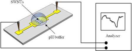
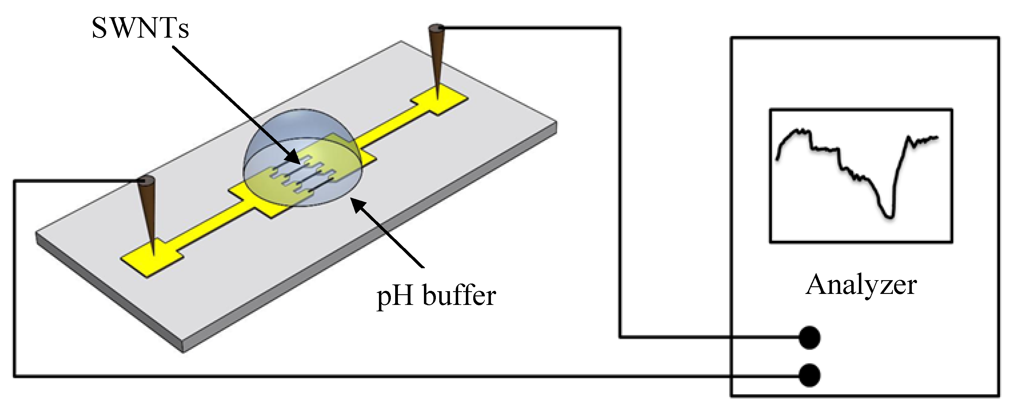
Because pH sensitivity measurement is conducted in an aqueous environment, a control experiment is needed to ensure that the majority of the charges transmit through the SWNTs instead of the solutions. In this experiment, the electrical conductivities of all the aqueous media—the pH buffer solutions and the DI water—are obtained by placing these solutions on open electrodes without the SWNTs. The semiconductor analyzer is used to measure the resistances of these solutions. The results show that the resistances of the solutions are almost infinite. This means that the solutions have much lower conductivities than the SWNTs. Therefore, for the SWNT-based pH sensors, the current is transmitted through the SWNTs almost exclusively. Any change recorded by the analyzer is caused by the resistance change of the SWNTs.
In our investigation, it is observed that the droplet placing and removing steps need to be performed a few times (10–15) before the sensor shows a stable response to pH solutions. We believe that during the first few instances of sensor wetting and drying, some SWNTs lose the connection with the electrodes and are washed away in the process. Therefore, only the initially strongly-bond SWNTs remain on the surface. The effect can be demonstrated by monitoring the SWNTs before and after the wetting and drying steps.
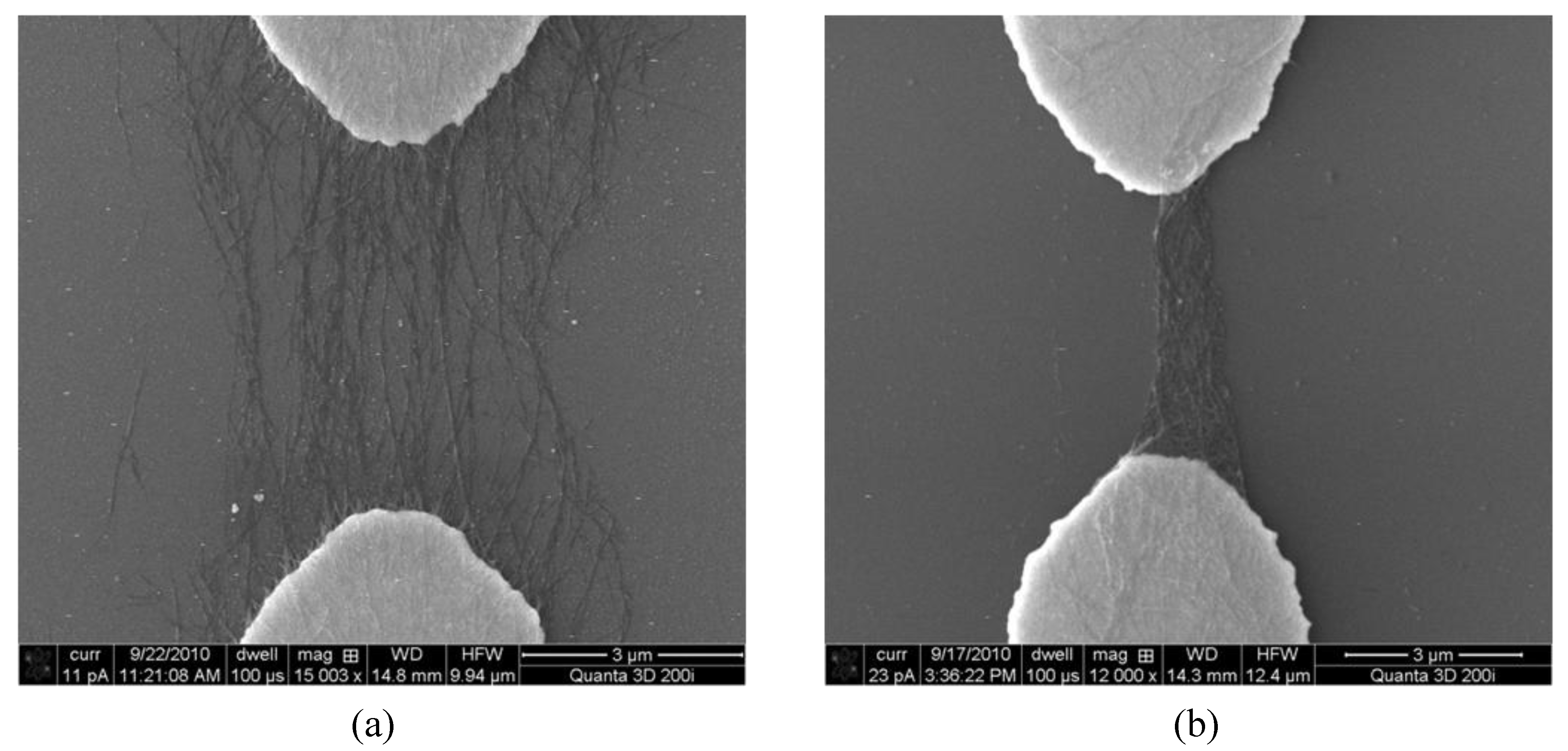
Figure 5(a) shows the aligned SWNTs right after the dielectrophoresis process but before the pH sensing steps. The SWNTs are sparsely distributed and loosely connected to the electrodes. In comparison,
Figure 5(b) shows the remaining SWNTs after a few instances of droplet placing and removing. The originally sparsely distributed SWNTs are now tightly congregated together and form a dense network. This is attributed to liquid surface tension when the solution residual evaporates. The surface tension pulls the SWNTs together and reinforces the connection between the SWNTs and the electrodes. In addition, the loosely-bond SWNTs are removed during the process. As a result, the sensor becomes more stable and demonstrates higher repeatability after these droplet placing and removing steps.
Figure 5.
(a) An SEM image of sparsely distributed SWNTs across the electrodes right after the dielectrophoresis deposition. (b) An SEM image of congregated SWNTs after the droplet placing and removing steps.
Figure 5.
(a) An SEM image of sparsely distributed SWNTs across the electrodes right after the dielectrophoresis deposition. (b) An SEM image of congregated SWNTs after the droplet placing and removing steps.
After the SWNTs become stabilized, the sensor is exposed to buffer solutions for pH sensitivity measurement. For each solution, a syringe is used to place a droplet on top of the SWNTs. During the measurement, the sensor is first exposed to the five solutions in the sequence of pH-9 to pH-5, and then it is exposed to the same solutions in the opposite sequence of pH-5 to pH-9.
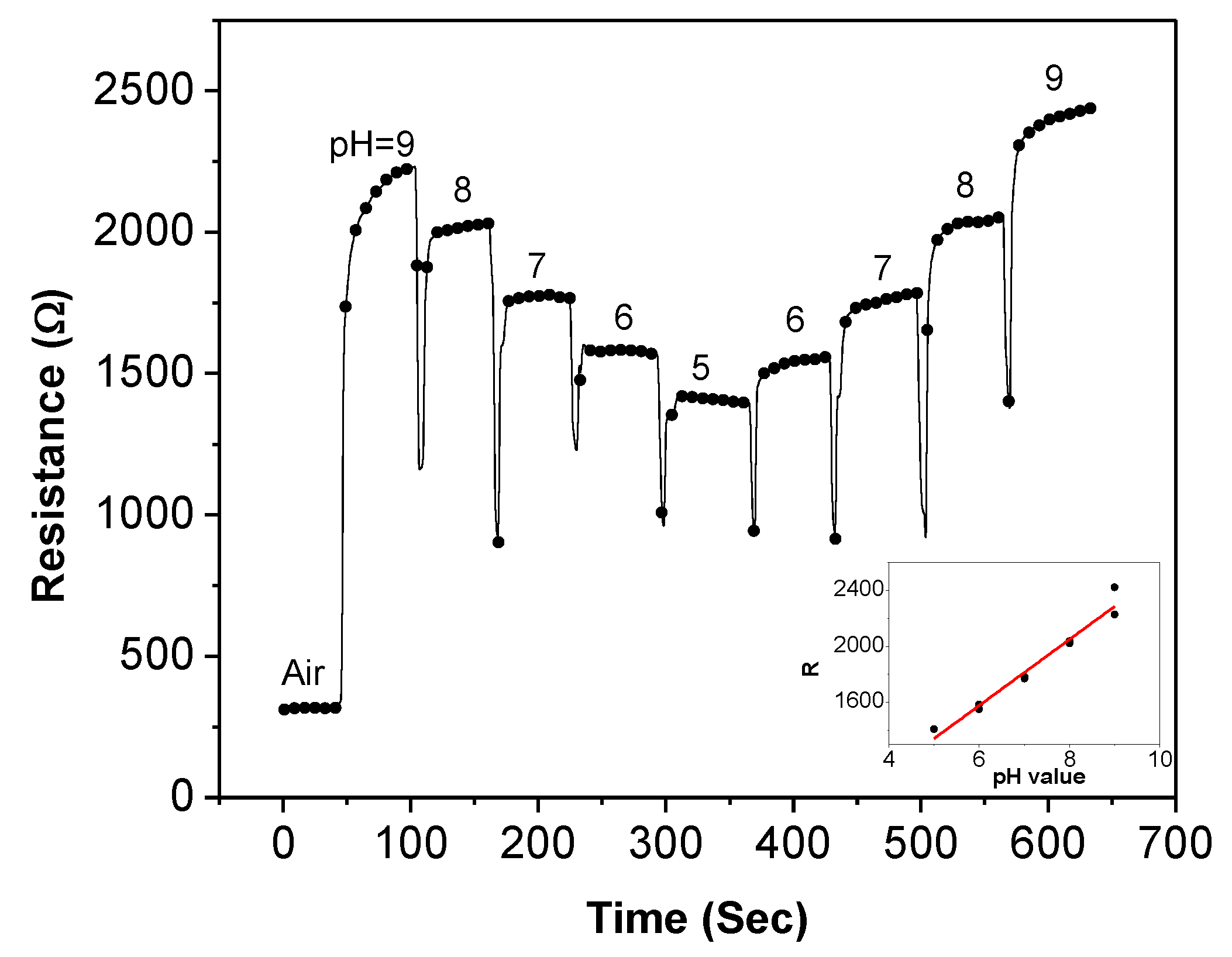
Figure 6 illustrates the recorded resistance history (resistance-time plot) of the sensor during the measurement. The real-time resistance change at different pH values proves that the sensor is highly sensitive to the pH variation. When the sensor is exposed to air, the resistance is approximately 316 Ω. After the pH-9 buffer is placed on the sensor, the resistance is rapidly increased to 2,226 Ω. The pH-9 buffer droplet is then removed after approximately 50 s when the sensor resistance is relatively stable. Next, the pH-8 buffer is dropped on the sensor immediately after the pH-9 buffer removal. The average sensor resistance is decreased by 206 Ω. The same step is repeated for pH-7, pH-6, and pH-5 solutions. Similar amount of decrement of sensor resistance can be observed for each step. On the other hand, almost equal amount of increment of sensor resistance is observed using the solutions with increasing pH values. Based on the recorded data, the sensor resistance and the pH values have a linear relationship of
R (Ω) = 236.3 × pH + 159, as shown in the inset of
Figure 6. This equation indicates that the absolute sensitivity of this particular sensor is 236.3 Ω/pH. However, we want to point out that even though the sensors are fabricated under the same condition, it is still challenging to deposit the exact same amount of SWNTs over the electrodes on every sensor. Consequently, the SWNT-based thin-film sensors often suffer from performance variation with absolute values vary from device to device. Another possible reason for the performance variation is from the material itself—SWNTs contain both metallic and semiconducting nanotubes. The uncertainty of the film composition causes the property variation of the deposited SWNTs. Therefore, a more consistent method needs to be used. In our investigation, the sensing repeatability and the normalized resistance of various sensors are used to characterize the performance of the SWNT-based sensors.
Figure 6.
The recorded resistance history of a SWNT-based sensor when exposed to pH buffers from pH-9 to pH-5 and then to pH buffers from pH-5 to pH-9.
Figure 6.
The recorded resistance history of a SWNT-based sensor when exposed to pH buffers from pH-9 to pH-5 and then to pH buffers from pH-5 to pH-9.
3.3. Sensing Repeatability
The sensing repeatability of the SWNT-based sensors is estimated through the measurement of five different sensors following the same procedure described above. All sensors demonstrate similar behaviors with resistance-time plots similar to the one shown in
Figure 6. The average resistance at each pH value is then calculated for each sensor. The normalized resistance is adopted to evaluate the sensor performance; it is defined as:
where
ΔR/Rr is the normalized sensor resistance,
ΔR is sensor resistance relative to the lowest sensor resistance,
Rr is the range of sensor resistance in the pH sensing test,
R is the absolute value of sensor resistance,
Rmax is the highest sensor resistance, and
Rmin is the lowest sensor resistance.
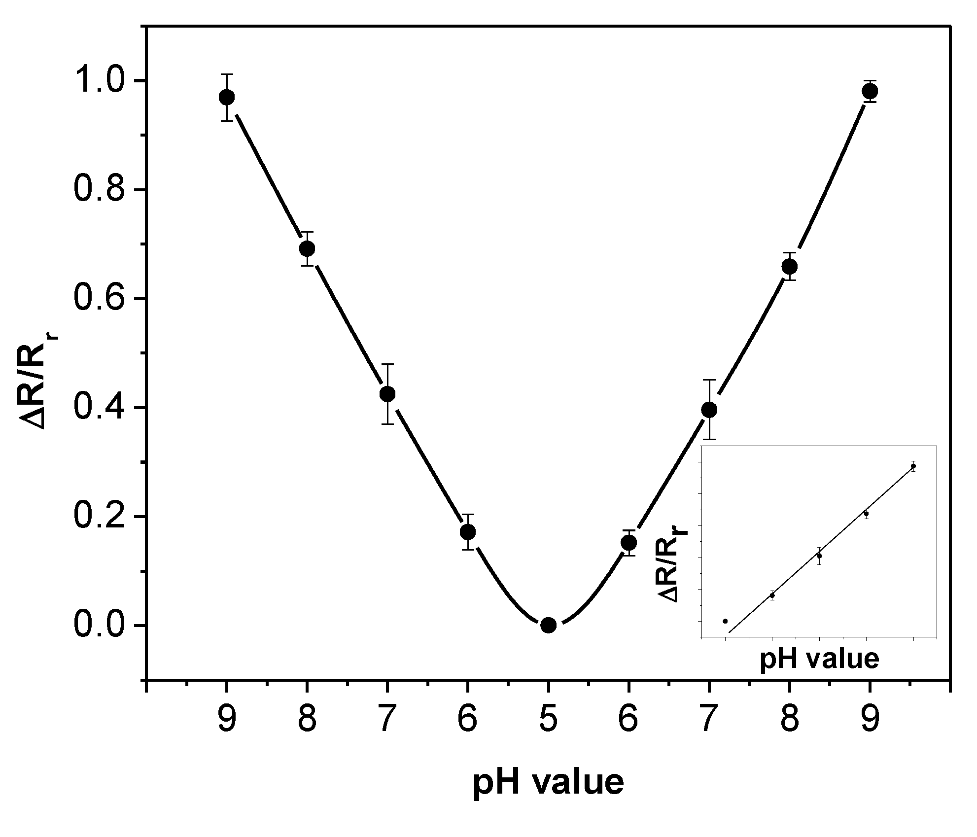
Figure 7 shows the average values (dots) and standard deviations (error bars) of the normalized resistances at different pH values for the five sensors. All the sensors follow the same trend of pH sensitivity and the values vary in a small range. This indicates that the pH sensitivity is highly repeatable for multiple sensors. As the pH value decreases from 9 to 5, the normalized sensor resistance drops proportionally. The opposite trend can be seen from the right half of the figure where the pH value increases. The figure also demonstrates that the sensor resistance depends solely on the pH value rather than the testing order of the pH solutions. The measurement data from the entire process are summarized and re-plotted as the inset of
Figure 7, which shows a linear relationship between the normalized sensor resistance and the pH values in the range of 5 to 9. The linear relationship can be described as:
This equation provides the calibration standard of the SWNT-based sensors using pH-5 to pH-9 buffer solutions.
Figure 7.
Normalized resistances versus pH values for five SWNT-based sensors. Inset: the linear relationship between the normalized sensor resistance and the pH value.
Figure 7.
Normalized resistances versus pH values for five SWNT-based sensors. Inset: the linear relationship between the normalized sensor resistance and the pH value.
3.4. Response Time
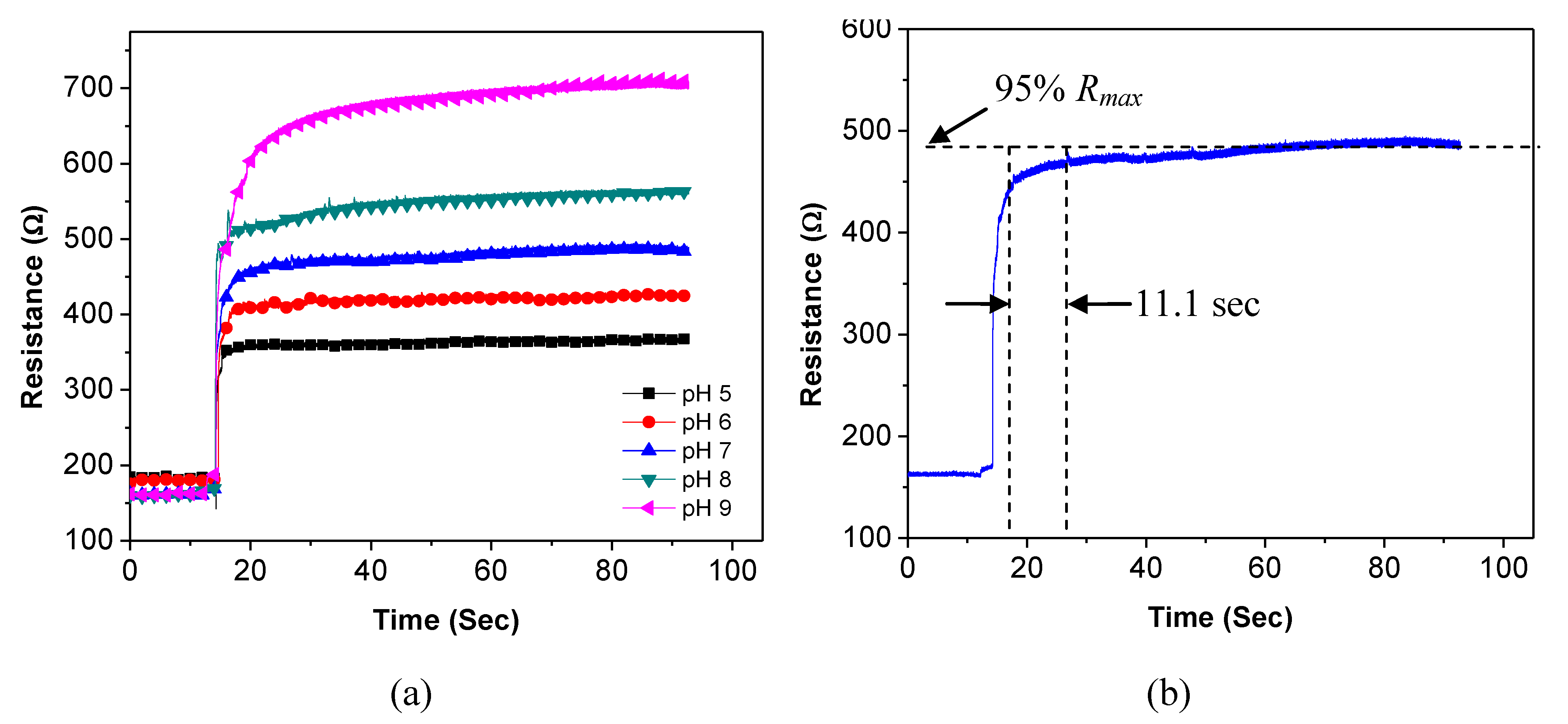
Response time represents how long it takes for the sensor to reach a steady state. To obtain accurate results, the response time of the sensor is investigated with an increased sampling rate of 100 points per sec. The initial resistance of the sensor in air is recorded by the analyzer. Next, a droplet of the pH buffer is placed on the sensor. After the resistance of the sensor reaches a stable value, the pH buffer is removed with the syringe. Next, the sensor is rinsed with DI water to remove the buffer residual. The same experiment is performed for all the pH buffer solutions and the results are illustrated in
Figure 8(a). All curves show instant increases after the buffer solutions cover the sensor. The pH-5 buffer yields the minimum sensor resistance. As the pH value increases, the resistance of the sensor increases. In addition, the measurement results show that the response time of the sensor is not a constant; instead, it depends on the pH value. In our investigation, the response time of the sensor is defined as the time for the resistance to reach 95% of its maximum value. An example curve is illustrated in
Figure 8(b) for the pH-7 buffer. It takes the sensor 11.1 s for its resistance to reach 95% of the maximum value of 495 Ω.
Figure 8.
(a) pH response under buffer solutions from pH-5 to pH-9. (b) The response time of the sensor under the pH-7 buffer solution.
Figure 8.
(a) pH response under buffer solutions from pH-5 to pH-9. (b) The response time of the sensor under the pH-7 buffer solution.
Using the same method, the sensor response times at different pH values are calculated and summarized in
Table 1. The sensor response time increases when the pH value increases. The pH-dependent response time may be caused by the interaction speed between the hydrogen ions and the SWNTs. As the concentration of hydrogen ions becomes lower, the protonation/deprotonation process becomes slower. Consequently, it takes longer time for the SWNTs to reach a stable resistance.
Table 1.
Sensor response time under different pH values.
Table 1.
Sensor response time under different pH values.
| pH value | 5 | 6 | 7 | 8 | 9 |
|---|
| Response time (s) | 2.26 | 3.08 | 11.1 | 17.05 | 23.82 |
3.5. Long-Term Stability
Long-term stability is an important parameter for sensors, especially for pH sensors because they are used in aqueous environments which usually contain many affecting factors. Ideally, the sensors should be able to maintain their sensitivity for a long period of time. To study the long-term stability, a SWNT-based sensor is characterized every 24 h for 10 consecutive days under the same experimental conditions.
Figure 9(a) shows the recorded absolute resistances of the sensor in different pH buffer solutions during this period. The values are relatively stable. The sensor remains sensitive to the pH buffer solutions after 10 days; and its sensitivity is relatively consistent during this period. To estimate the relationship between the absolute resistance and the pH value, the obtained data are re-plotted in
Figure 9(b). The dots represent the average values and the error bars represent the standard deviations of the sensor resistance. The resistance-pH plot verifies that the sensor maintains its linear relationship between the resistance and the pH values during the 10-day period.
Figure 9.
Resistance variation of one sensor in five pH buffer solutions in 10 days.
Figure 9.
Resistance variation of one sensor in five pH buffer solutions in 10 days.


