A Localized Meshless Technique for Generating 3-D Wind Fields

Abstract

A localized meshless method is used to simulate 3-D atmospheric wind fields for wind energy assessment and emergency response. The meshless (or mesh-free) method with radial basis functions (RBFs) alleviates the need to create a mesh required by finite difference, finite volume, and finite element methods. The method produces a fast solution that converges with high accuracy, establishing 3-D wind estimates over complex terrain. The method does not require discretization of the domain or boundary and removes the need for domain integration. The meshless method converges exponentially for smooth boundary shapes and boundary data, and is insensitive to dimensional constraints. Coding of the method is very easy and can be done using MATLAB or MAPLE. By employing a localized RBF procedure, 3-D wind fields can be established from sparse meteorological data. The meshless method can be easily run on PCs and hand-held mobile devices. This article summarizes previous work where the meshless method has successfully simulated 3D wind fields over various environments, along with the equations used to obtain the simulations.

1. Introduction

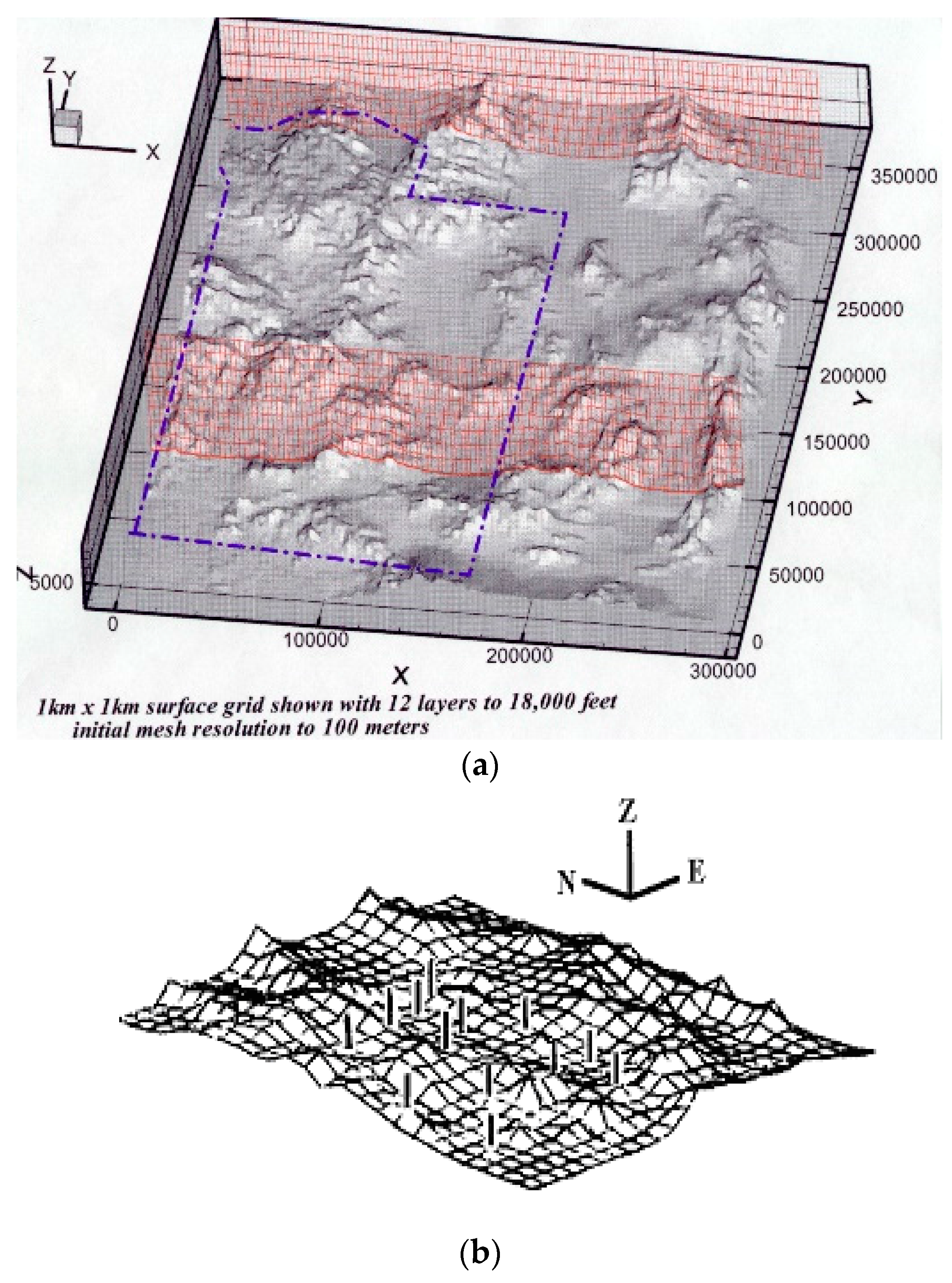
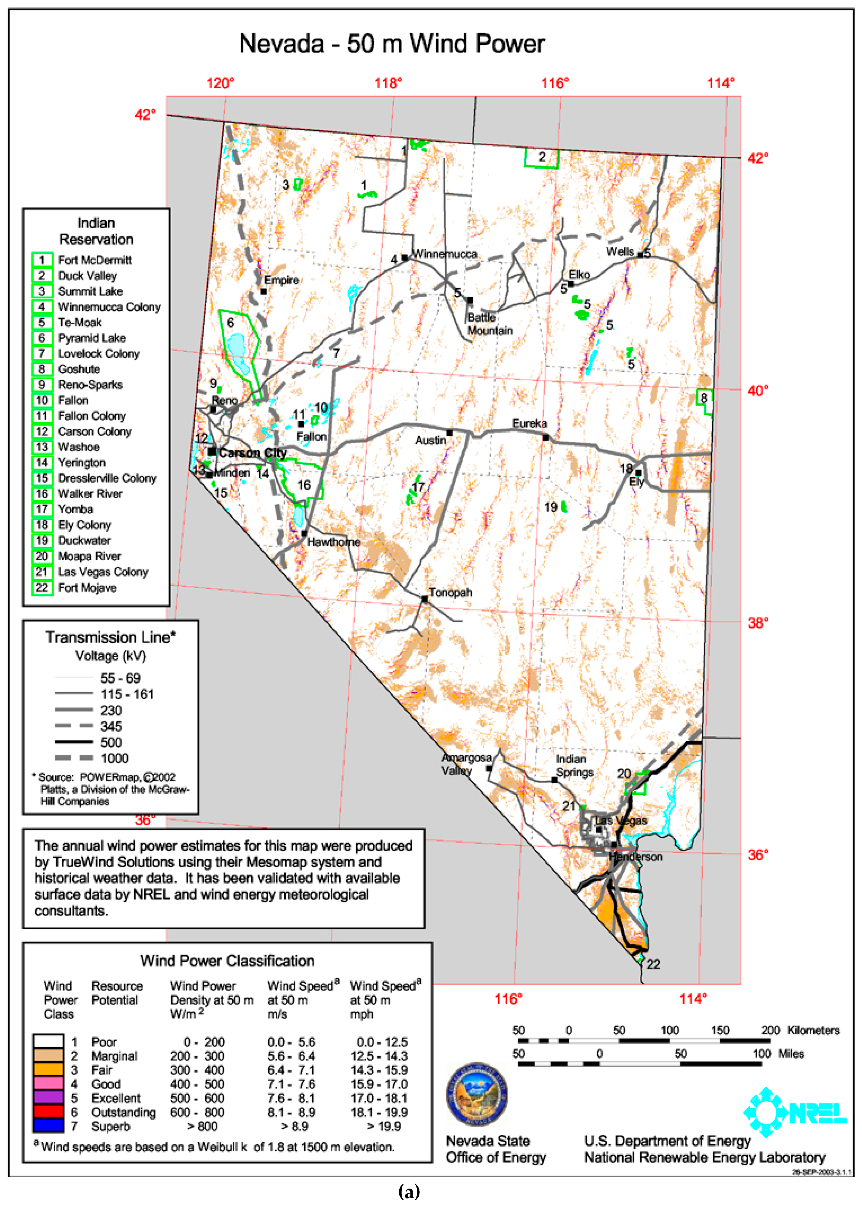
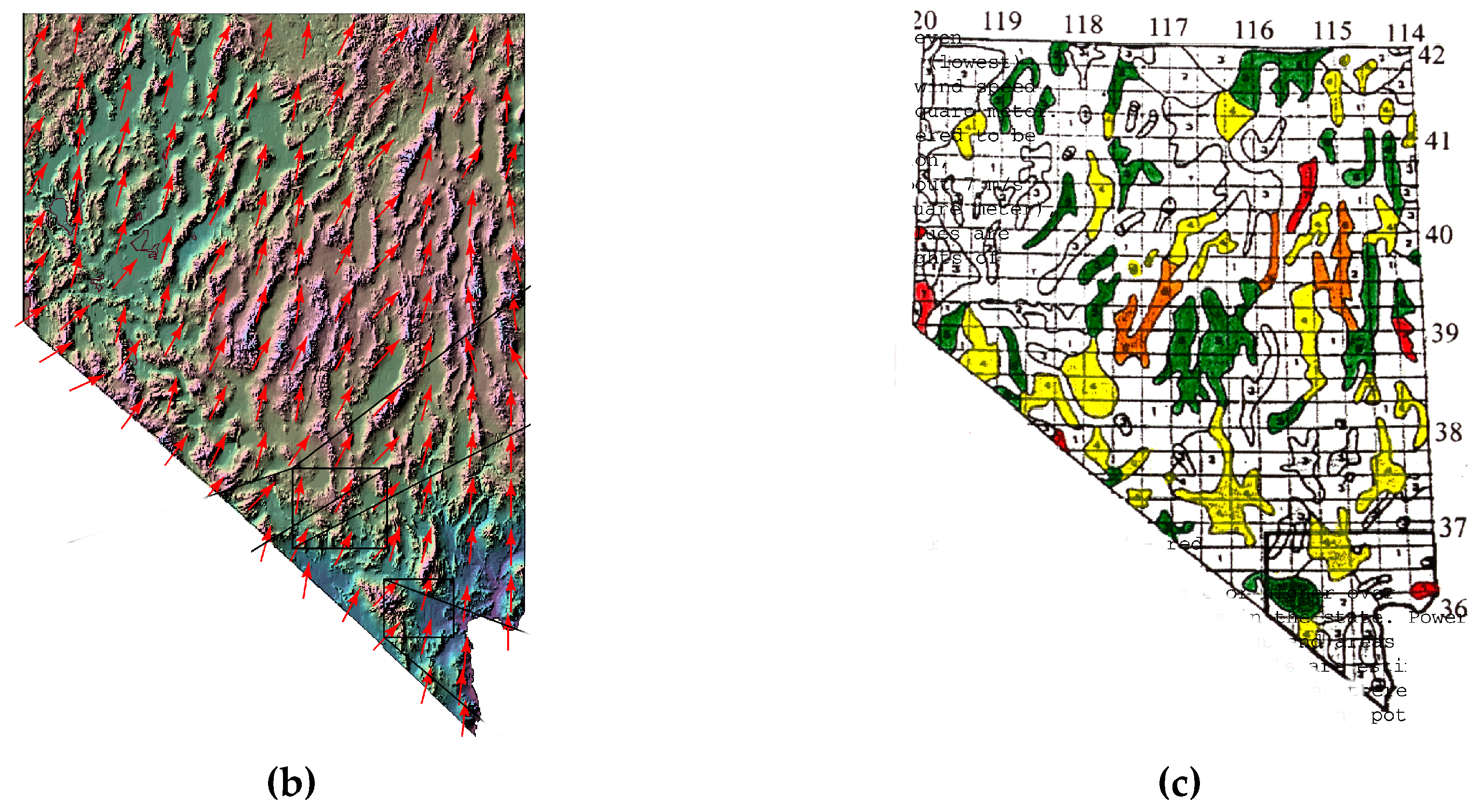
Wind energy continues to be a limited resource in the Southwestern U.S. A preliminary wind energy study conducted by Pepper [1] and later by the National Renewable Energy Laboratory (NREL) and AWS Truewind (now AWS Truepower, Albany, NY, USA) [2] showed that Nevada has wind resource potential (Figure 1a). Detailed wind energy resource data is difficult to obtain, requiring data gathering equipment to reach remote ridges and mountain tops where higher-class winds may exist. Previous efforts indicated that Nevada has significant wind resource potential, mostly on ridge tops in rural areas [3]. Numerical simulations based on extensive mesh-based models are typically conducted to estimate the potential of wind energy over extended areas of interest. These models can be time consuming to setup and require extensive computational resources. A fast, alternative approach to these more conventional models is the use of meshless methods.

Sufficient wind resources may be available to provide both electric power and economic development opportunities for rural areas, as shown in Figure 1. Efforts were undertaken by the University of Nevada Las Vegas (UNLV) and Desert Research Institute (DRI) to examine wind energy potential within the central and upper Northern regions of the state. The UNLV-DRI study resulted in a revised, more refined estimate of wind resources within the central portion of the state with placement of four meteorological towers near Whitney Mountain.

2. Mass Consistent Winds

In order to create realistic 3-D wind fields, a mass consistent model must first be established. The basis for the model employed in this study follows the earlier works of Sherman [4] and later applied by Pepper [5]. The mass consistent model minimizes the differences between observed and computed velocity values. Simulation values are calculated at all the nodes within the computational domain utilizing weighted averaging around each measured meteorological data point, i.e., data obtained from an instrumented meteorological tower, to fill in values to all the nodes. This interpolated wind field is then minimized to reduce error and satisfy mass conservation. In this situation, the limitations of the incompressible approach should be noted. In reality, the atmosphere is compressible and the differences in density can lead to issues affecting temperature, humidity, and pressure (e.g., nocturnal drainage winds). In this approach, we have kept the simulations simple to provide quick estimates of the wind fields. A more detailed approach should include compressibility. However, the procedure would essentially be the same.

Inverse squared weighting is first used to create a preliminary surface wind field employing a fixed radius from the tower and the values interpolated to all grid points in the first level above the terrain. The remaining upper level winds are then constructed using inverse weighting from the initial surface generated values. If measured vertical velocities are not available, the equation of continuity is then used to calculate the remaining velocities, i.e.,

$$w=-{\displaystyle \underset{0}{\overset{z}{\int }}\left(\frac{\partial u}{\partial x}+\frac{\partial v}{\partial y}\right)}dz$$

(1)

which stems from the conservation of mass for atmospheric (incompressible) flow [6],

$$\frac{\partial u}{\partial x}+\frac{\partial v}{\partial y}+\frac{\partial w}{\partial z}=0$$

(2)

A variational technique originally employed by Sasaki [7] is used to create an equation for Lagrange multipliers, $\lambda \left(x,y,z\right),$ which are used to adjust velocities. This Poisson equation contains the observed velocity values (u₀, v₀, and w₀ obtained from meteorological tower or SODAR-SOnic Detection and Ranging-data), along with Gauss moduli (α) that can be tuned to adjust for more horizontal or vertical effects (e.g., rough terrain may create more vertical influence). The resulting Euler-Lagrange equation for $\lambda \left(x,y,z\right)$ written as

$$\frac{{\partial }^2\lambda }{\partial x^2}+\frac{{\partial }^2\lambda }{\partial y^2}+{\left(\frac{{\alpha }_1}{{\alpha }_2}\right)}^2\frac{{\partial }^2\lambda }{\partial z^2}=-2{\alpha }_1^2\left(\frac{\partial u_0}{\partial x}+\frac{\partial v_0}{\partial y}+\frac{\partial w_0}{\partial z}\right)$$

(3)

where $u_0, v_0, w_0$ are the measured velocity values in the x, y, and z directions and α_i are the Gauss precision moduli, where α_i²≡ 1/(2σ_i²) (with the deviation errors from the observed and desired fields defined by σ_i). Sherman [4] points out that these moduli are important in establishing non-divergent wind fields over irregular terrain, where (α₁/α₂)² is proportional to (w/u)². Pepper and Wang [8] set α₁ (the horizontal adjustment) = 0.01 and α₂ (the vertical adjustment) = 0.1.

Once λ is calculated at each node, the velocities are adjusted to satisfy continuity, keeping the measured tower velocities fixed, i.e.,

$$u=u_0+\frac{1}{2{\alpha }_1^2}\frac{\partial \lambda }{\partial x}$$

(4)

$$v=v_0+\frac{1}{2{\alpha }_1^2}\frac{\partial \lambda }{\partial y}$$

(5)

$$w=w_0+\frac{1}{2{\alpha }_2^2}\frac{\partial \lambda }{\partial z}$$

(6)

Measured velocities are typically collected and averaged every 10–15 min, generating a new 3-D wind field. Equations (3)–(6) are updated once per cycle. Setting λ = 0 accounts for open or “flow-through” boundaries; setting ∂λ/∂n = 0 on the boundary defines closed or “no-flow-through” boundaries. Both Sherman [4] and Dickerson [9] employed this technique to produce realistic wind fields using very sparse measured values.

3. Wind Power Density Calculation

Wind power density ranges from Class 1 (lowest) to Class 7 (highest), defined on a vertical extrapolation of wind speed based on the 1/7 power law. The Battelle Wind Energy Resource Atlas provides the source for classification data [10]. Satisfactory power-generating winds are typically Class 4 winds and higher, but as wind turbine technology advances, Class 3 winds are becoming viable.

Table 1. Wind Class versus Power Density.

Class	Power Density (W/m2)	Mean Speed(m/s)
1	<200	<5.6
2	200–300	5.6–6.4
3	300–400	6.4–7.0
4	400–500	7.0–7.5
5	500–600	7.5–8.0
6	600–700	5.6–8.8
7	>800	>8.8

shows wind class versus power density for winds at 50 m.

The wind power density calculations are obtained by calculating the wind speed at each grid point on an hourly basis.

$$Spee{d}_i=\sqrt{u_i^2+v_i^2+w_i^2}$$

(7)

The hourly wind power density at each grid point is then obtained using the simple expression,

$$WP{D}_i=0.5·\rho ·Spee{d}_i^3$$

(8)

with wind power in Watts, area is m², wind velocity is m/s, and the density for air is 1.225 kg/m³ at sea level. To account for density variation at elevation Z (above sea level in m), density is obtained using

$$\rho =1.225-(1.194\times {10}^{-4})·Z$$

(9)

The monthly average wind power density is then calculated using the relation

$$WP{D}_{monthly\_avg}=\frac{{\displaystyle \sum _{i=1}^{N}WP{D}_i}}{N}$$

(10)

where N is the total number of hours in a selected month.

4. The Meshless Method

The meshless method is a unique numerical technique that does not require discretization with a mesh [11,12]. In addition, the method can easily handle complex geometrical problems with inhomogeneous or variable properties employing a general-purpose algorithm. Applications of meshless (or mesh-free) methods have continued to increase over the past few years to solve a wide range of problems [13,14,15,16]. In many situations, the meshless method can serve as a viable alternative to problems involving complex or extensive mesh generation. Atluri and Zhu [13,17,18] discuss the issue of node placement in mesh-free methods. In this work, radial basis functions (RBF) are used since issues dealing with nodal placement are not critical.

The concept of a meshless approach to obtain approximate solutions to differential equations began in the 1970s [19]. The method began to take more notice in the ensuing years due to their ease in implementation, bypassing the need for nodal connectivity required in the more widely used conventional mesh-based numerical methods. Mesh discretization using finite elements as well as non-structured polygonal mesh techniques used in finite volume methods can become troublesome when encountering complex geometries. While a variety of meshless approaches now exist, they have the common property of not requiring a nodal mesh. This is a unique feature of the method, and truly eliminates the effort typically required to produce a refined and optimal mesh (to ensure mesh independence solutions including refined local adaptations—both time consuming). The more common forms of meshless methods include smoothed particle hydrodynamics, reproducing kernel particle, meshless Petrov–Galerkin, local radial point interpolation, finite point, and finite differences with arbitrary irregular grids. Each method has benefits and drawbacks. Further details describing the unique properties of meshless methods are given in Liu [15].

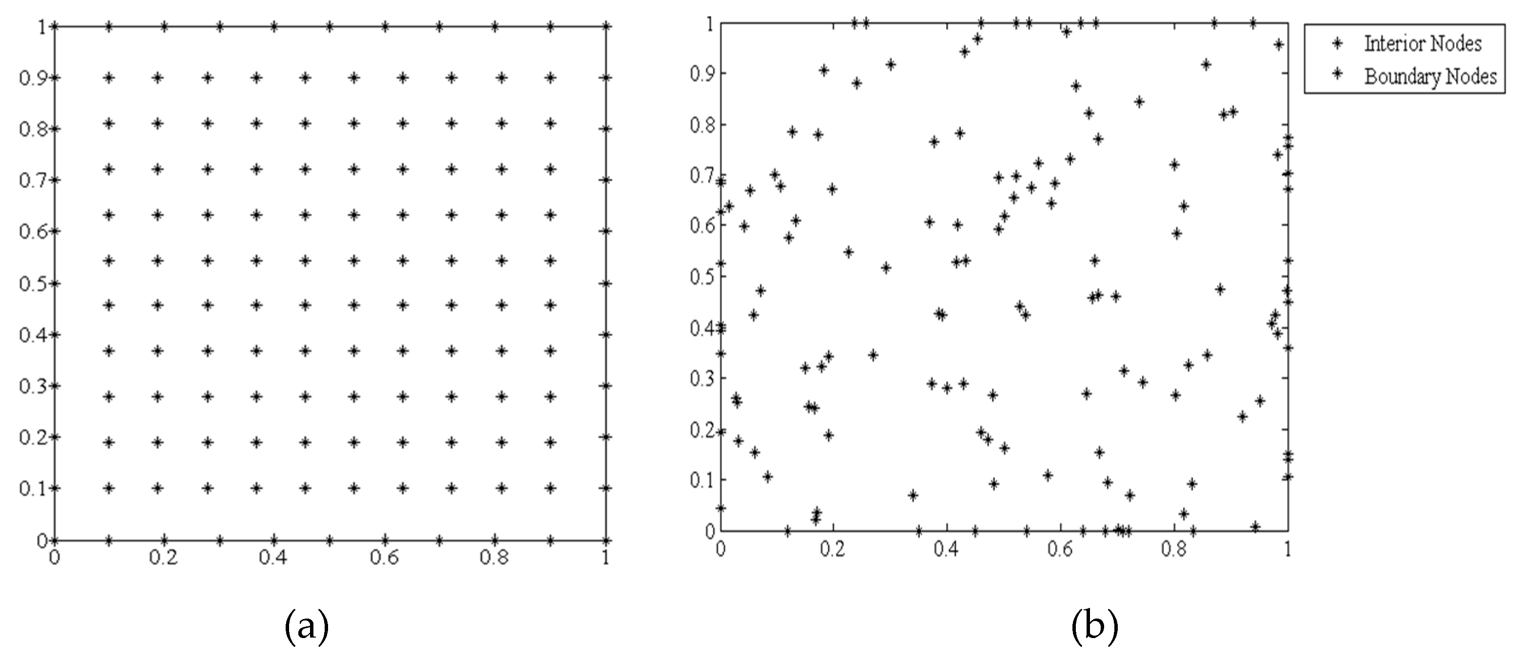
An example illustrating the placement of nodes in a uniform pattern versus a random pattern is shown in Figure 2a,b. The nodes do not need to be distributed uniformly, and in fact can be scattered and grouped within the problem domain to more accurately capture information in regions of greater interest.

Shape functions relate the influences from all the nodes within the domain on each individual node. These functions act as support domains for each node, and can have weighted influence. In this instance, the Lagrange multipliers, $\lambda \left(x\right)$, are interpolated using the displacements at their nodes within the support domain. For example, a PDE is discretized into a nodal matrix form, and the global matrix solved using a simple elimination procedure.

4.1. Radial Basis Functions (RBF)

The RBF method employs a basis function that relates the influence of surrounding nodes to the node of interest, i.e., a distance, d, with the nodes closest to the node of interest having the greatest influence. This distance between the radial positions, r, can be expressed as:

$$d_i={\left[{\left(r-r_i\right)}^2\right]}^{1/2}$$

(11)

Hardy [20] introduced a basis function based on multi-quadratics (MQ). The MQ is a popular function used to construct approximate solutions to PDEs, and is used in this study. Incorporating the relation for distance, a basis function, ϕ, can be established such that:

$${\varphi }_j={\left[{\left(r-r_j\right)}^2+c_j^2\right]}^{1/2},j=1,2\dots N$$

(12)

where N is the total number of nodes. The Lagrange multipliers, $\lambda \left(x\right)$, are then expressed as:

$$\lambda (x)={\displaystyle \sum _{j=1}^N{\varphi }_j}(x){\lambda }_j$$

(13)

where λ_j is the Lagrange coefficient defined at each point.

In order to solve the Poisson equation for λ(x), a linear operator ($L\equiv {\nabla }^2$) is applied to the interior domain, Ω. Thus,

$$L\lambda (x)={\displaystyle \sum _{j=1}^{N}L{\varphi }_j(x)}{\lambda }_j$$

(14)

where the linear operator (the PDE) is applied to the basis function. First and second derivatives of the basis function are used to solve Equation (3). A boundary operator, B, is used to account for either Dirichlet or Neumann conditions applied to the boundaries, Γ, i.e.,

$$B\lambda (x)={\displaystyle \sum _{j=1}^{N}B{\varphi }_j(x){\lambda }_j}$$

(15)

The procedure used in this study is based on the approach used by Kansa [21]. Note that different constants for the shape parameter can be used for the interior, Ω, and the boundary, Γ.

Equation (3) can be expressed as:

$$\frac{{\partial }^2\lambda }{\partial x^2}+\frac{{\partial }^2\lambda }{\partial y^2}+{\left(\frac{{\alpha }_1}{{\alpha }_2}\right)}^2\frac{{\partial }^2\lambda }{\partial z^2}=f(x)x\in \mathsf{\Omega }$$

(16)

where x ≡ (x,y,z) with

$$f(x)=-2{\alpha }_1^2\left(\frac{\partial u_0}{\partial x}+\frac{\partial v_0}{\partial y}+\frac{\partial w_0}{\partial z}\right)$$

(17)

at all interior points, and

$$\lambda (x)=g(x)x\in \mathsf{\Gamma }$$

(18)

where g(x) denotes the divergence of the observed velocity values at the boundaries, Г. Introducing the MQ form of the basis function for ${\varphi }_j(x)$,

$${\varphi }_j(x)=\sqrt{r_j^2+c^2}=\sqrt{{(x-x_j)}^2+{(y-y_j)}^2+{(z-z_j)}^2+c^2}$$

(19)

the derivatives can be written as

$$\begin{array}{l}\frac{\partial {\varphi }_j}{\partial x}=\frac{x-x_j}{\sqrt{r_j^2+c^2}},\frac{\partial {\varphi }_j}{\partial y}=\frac{y-y_j}{\sqrt{r_j^2+c^2}},\frac{\partial {\varphi }_j}{\partial z}=\frac{z-z_j}{\sqrt{r_j^2+c^2}}\\ \frac{{\partial }^2{\varphi }_j}{\partial x^2}=\frac{{(y-y_j)}^2+{(z-z_j)}^2+c^2}{\sqrt[3]{r_j^2+c^2}},\frac{{\partial }^2{\varphi }_j}{\partial y^2}=\frac{{(x-x_j)}^2+{(z-z_j)}^2+c^2}{\sqrt[3]{r_j^2+c^2}},\frac{{\partial }^2{\varphi }_j}{\partial z^2}=\frac{{(x-x_j)}^2+{(y-y_j)}^2+c^2}{\sqrt[3]{r_j^2+c^2}}\end{array}$$

(20)

Substituting Equation (20) into Equations (16) and (18),

$${\displaystyle \sum _{j=1}^N\left(\frac{{\partial }^2{\varphi }_j(x_i)}{\partial x^2}+\frac{{\partial }^2{\varphi }_j(x_i)}{\partial y^2}+{\left(\frac{{\alpha }_1}{{\alpha }_2}\right)}^2\frac{{\partial }^2{\varphi }_j(x_i)}{\partial z^2}\right)}{\lambda }_j(x_i)=f(x_i)i=1,2,\cdots ,N_I$$

(21)

$${\displaystyle \sum _{j=1}^N{\varphi }_j(x_i}){\lambda }_j=g(x_i)i=N_{I+1},N_{I+2},\cdots N$$

(22)

an N × N linear system of equations is created for the unknown, λ_j.

The introduction of the shape parameter, c, assists in enhancing the accuracy of the RBFs. The shape parameter is based on the number of nodes, N, and distance, d, where $d=\frac{1}{N_I}{\displaystyle \sum _{i=1}^N{d}_i}$, and d_i is the distance between the i th data point and its nearest neighbor. The shape parameter depends on the number and distribution of nodes, the choice of basis function, and computer precision [22].

4.2. Local RBF Approach

The two techniques commonly used in RBF-based methods are based on global versus local collocation. The global approach collocates over the total number of nodes within the computational domain, i.e., the global matrix is defined by the total number of nodes, N, creating an N × N matrix that must be solved. The local approach employs only local collocation, creating a series of overlapping matrices defined by m x m nodes surrounding the node of interest. This creates a small series of linear equations that must be solved for each node. Providing the problem domain and number of nodes are not huge, the global RBF approach works well for simple and small problems. Pepper et al. [23] describes the use of the global RBF approach for 3-D wind fields. More detailed discussion on implementation of the local approach is given in Waters and Pepper [24]. Since the localized RBF method collocates a small number of points for each subdomain, the method is ideal for use as an app on mobile devices.

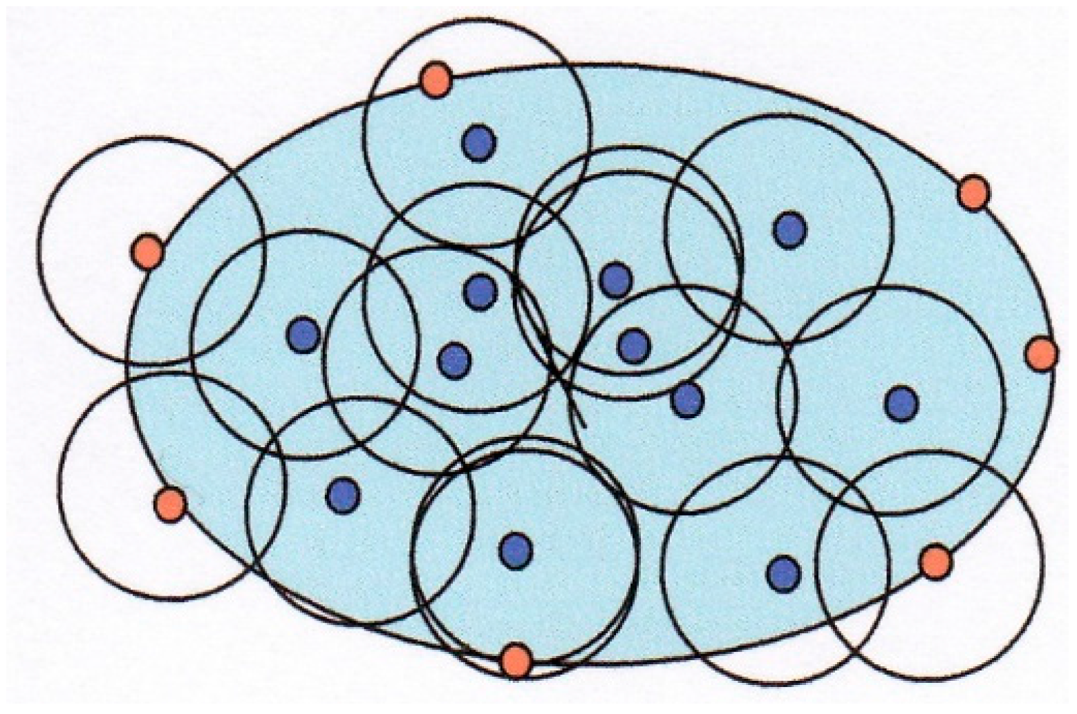
In order to approximate λ(x) of Equation (16), a series of local subdomains are solved that overlap within the problem domain. Figure 3 shows a set of subdomains with the dark points serving as the center node points. Each node serves as a center node of interest until all the nodes are resolved. This permits λ(x) to be solved at every point, i.e.,

$$\lambda (x_i)={\displaystyle \sum _{k=1}^m{\varphi }_k(x_i}){\lambda }_{k,j},x_i\in {\mathsf{\Omega }}_j$$

(23)

where λ_k,j are the coefficients of the RBFs. The RBF, ${\varphi }_k$, are the shape functions. Substituting Equation (23) into Equation (21), an m x m linear algebraic system is obtained for each local domain with an interior point, i.e.,

$${\displaystyle \sum _{k=1}^m\left(\frac{{\partial }^2{\varphi }_k(x_i)}{\partial x^2}+\frac{{\partial }^2{\varphi }_k(x_i)}{\partial y^2}+{\left(\frac{{\alpha }_1}{{\alpha }_2}\right)}^2\frac{{\partial }^2{\varphi }_k(x_i)}{\partial z^2}\right)}{\lambda }_{k,j}(x_i)=f(x_i)i=1,2,\cdots ,m{x}_i\in {\mathsf{\Omega }}_j$$

(24)

with the boundary conditions:

$${\displaystyle \sum _{k=1}^m{\varphi }_k(x_i){\lambda }_{k,j}(x_i)=g(x_i})i\in N_{I+1},N_{I+2},\cdots ,N{x}_i\in {\mathsf{\Omega }}_j$$

(25)

An m × m linear system consisting of the unknown multipliers, ${\left\{{\lambda }_{k,j}\right\}}_{k=1}^m$ is produced from Equations (24) and (25) for each local domain defined by the interior center points where Equation (24) applies to interior points $\left(x_i, i=1,2,\dots ,N_I\right)$ and Equation (25) applies to the boundary points.

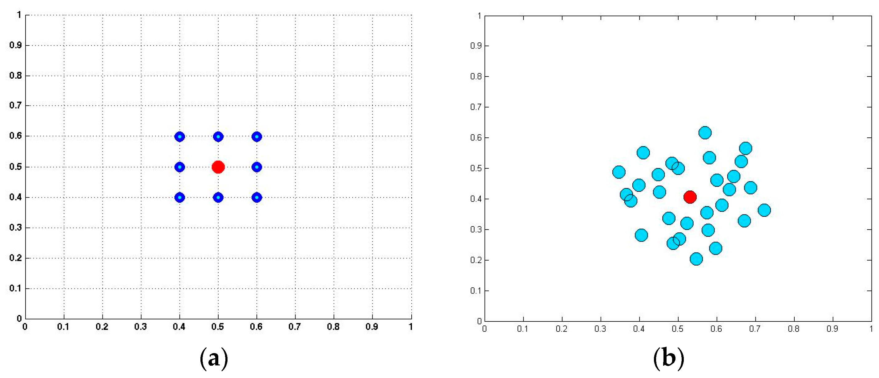
Figure 4a,b shows a localized domain on a simple rectangular field with the center point surrounded by 8 nodes, and a randomized array consisting of 30 points. Various test cases were examined as to the optimal number of surrounding nodes, ranging from 5 to 30. It was found that the best number with regards to acceptable accuracy and speed was nine nodes per local domain. The global matrix involving N × N nodes in the global technique reduces to a simple m × m matrix that can be quickly solved, and does not create matrix conditioning issues.

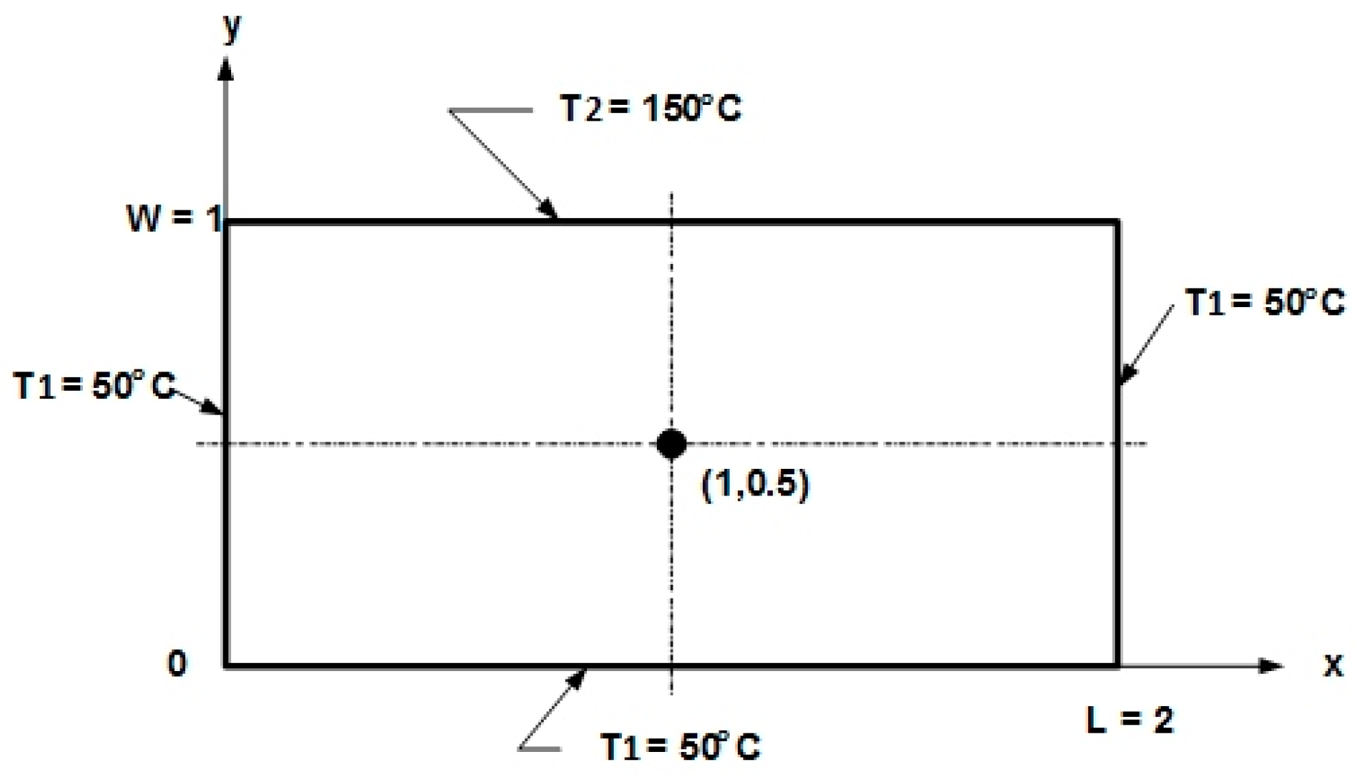
As an example, to illustrate the accuracy of the meshless method, a simple test case was used to solve for heat conduction in a two-dimensional plate subjected to prescribed temperatures along each boundary [25], as shown in Figure 5. The temperature at the mid-point (1,0.5) was used to compare numerical solutions with the analytical solution. The analytical solution is given as

$$\theta (x,y)\equiv \frac{T-T_1}{T_2-T_1}=\frac{2}{\pi }{\displaystyle \sum _{n=1}^{\theta }\frac{{(-1)}^{n+1}+1}{n}}\sin \left(\frac{n\pi x}{L}\right)\frac{\sinh (n\pi y/L)}{\sinh (n\pi W/L)}$$

which yields θ(1,0.5) = 0.445, or T(1,0.5) = 94.5 °C.

Table 2. Comparison of results for Exact, FEM, and Meshless Method (from Pepper, D.W., et al. [25]).

Method	Mid-Point (°C)	Elements	Nodes
Exact	94.512	0	0
FEM	94.605	256	289
Meshless	94.514	0	325

lists the final exact temperatures at the mid-point compared with a finite element and the meshless method.

5. Comparison Results

The Nevada Test Site (NTS) is located within the southern part of Nevada, about 100 miles northwest of Las Vegas. The NTS was used principally for nuclear weapons testing. The terrain and 26 wind tower locations are shown in Figure 6.

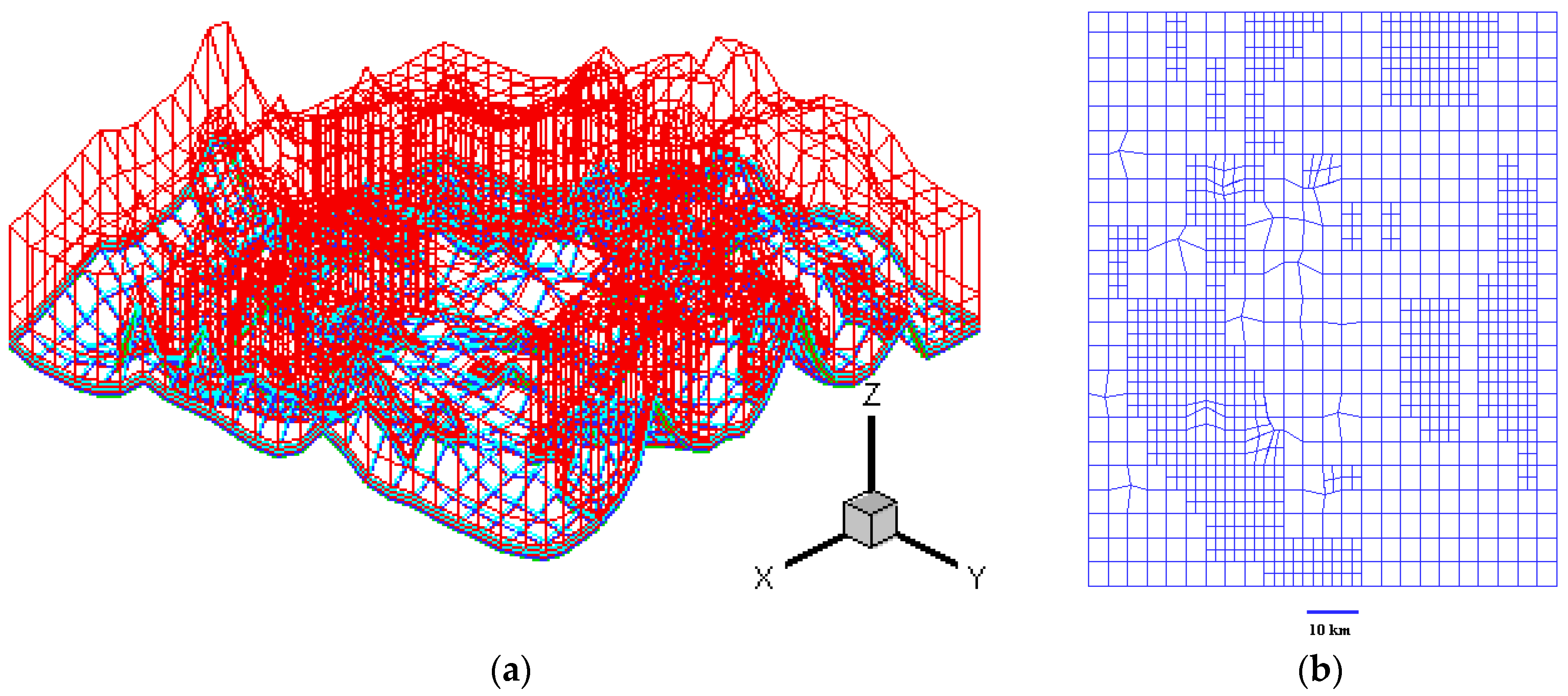
An h-adaptive finite element model was initially developed by Pepper and Wang [8] utilizing the UNLV supercomputer system to simulate 3-D winds over the NTS, as shown in Figure 6. The initial meshes were constructed using USGS and DEM data.

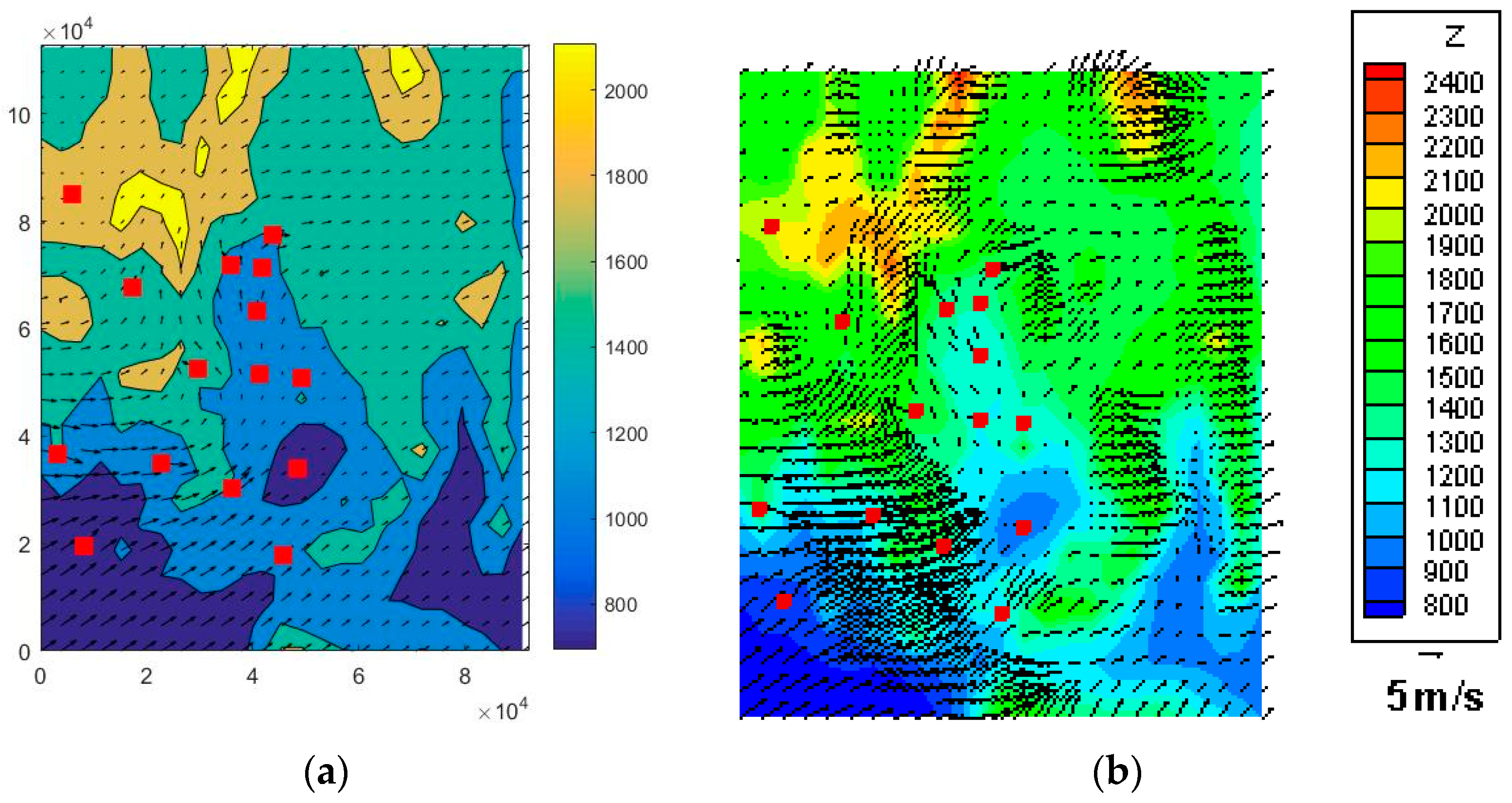
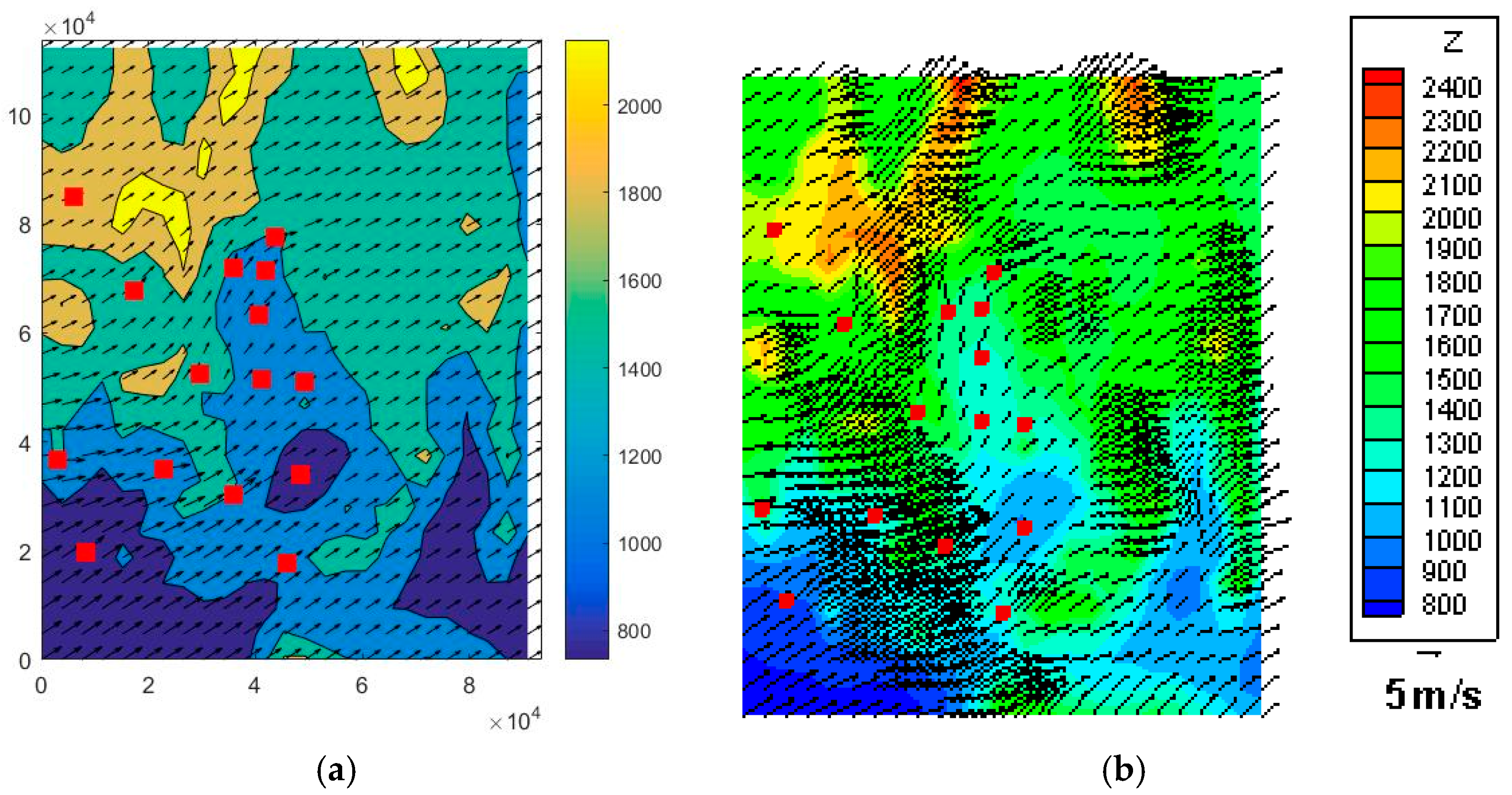
Meteorological tower and upper air data from 1 January 1993, were used to initialize the wind field. The NTS meteorological towers (partially shown as dots in Figure 6b are scattered throughout the site. The 10 m level mesh is shown in Figure 7a,b for the h-adaptive FEM model. The additional velocity vectors in the FEM solution in Figure 8b occur from local refinement (h-adaptation). 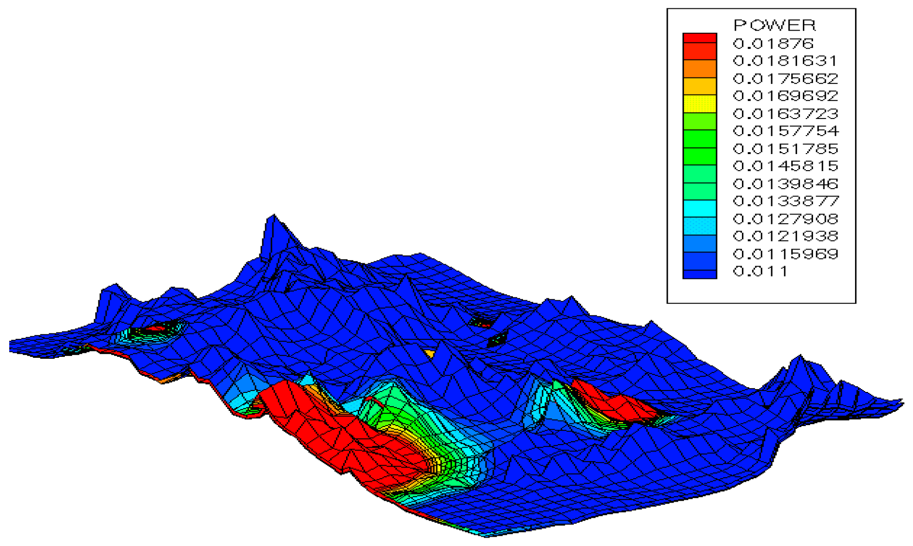Results for the 50 m level are shown in Figure 9a,b. A power density map of the NTS is shown in Figure 10.

The meshless method employed only 240 nodes. The FEM model required over 12,500 nodes. While the meshless method utilized a coarse density of nodes, the velocities and patterns were generally close to the results obtained using the high-resolution finite element model. Furthermore, the meshless code was written in MATLAB, a widely popular and inexpensive software package used in many institutions than runs on PC platforms, while the h-adaptive FEM was written in FORTRAN, parallelized, and was run on a supercomputer.

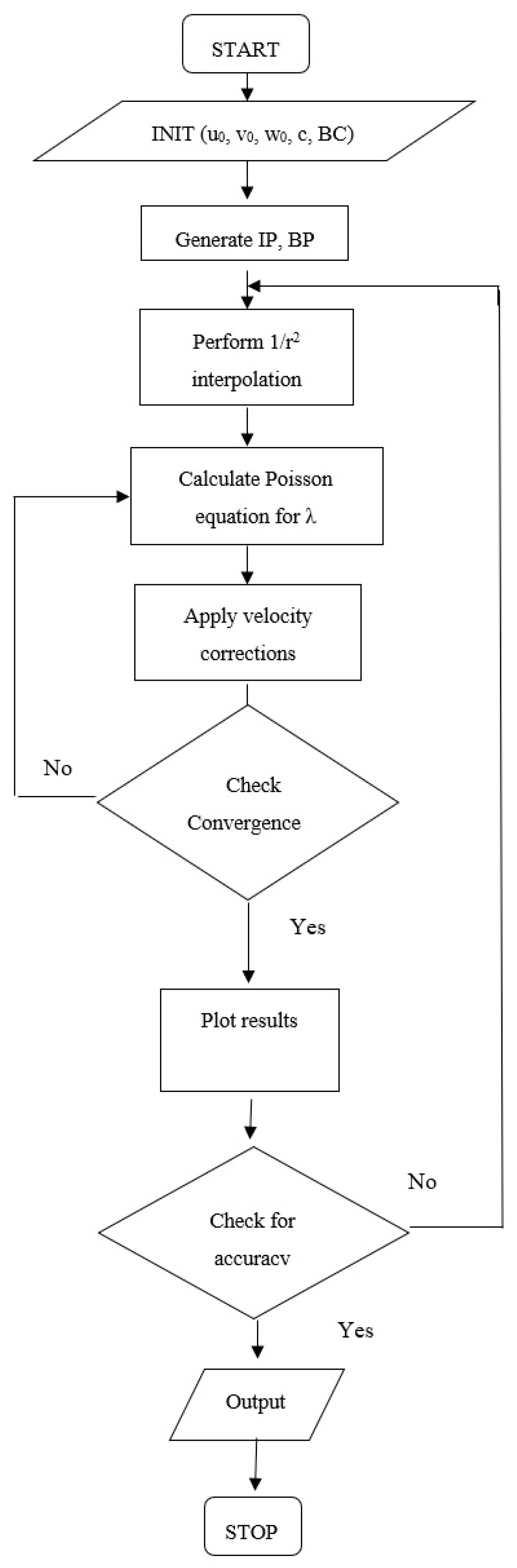
A simple flow chart is listed in Figure 11 for generating the model output. The implementation of the coding is very simple, especially since the method is explicit and does not require matrix solvers.

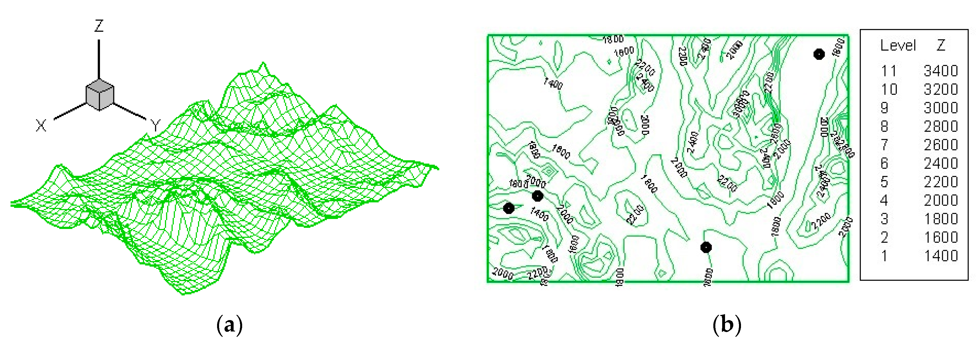
Later efforts were undertaken to examine wind energy potential for central NV. The terrain surface plot, topographic contours, and tower locations are shown for the region near Whitney Mountain in central NV in Figure 12a,b [26].

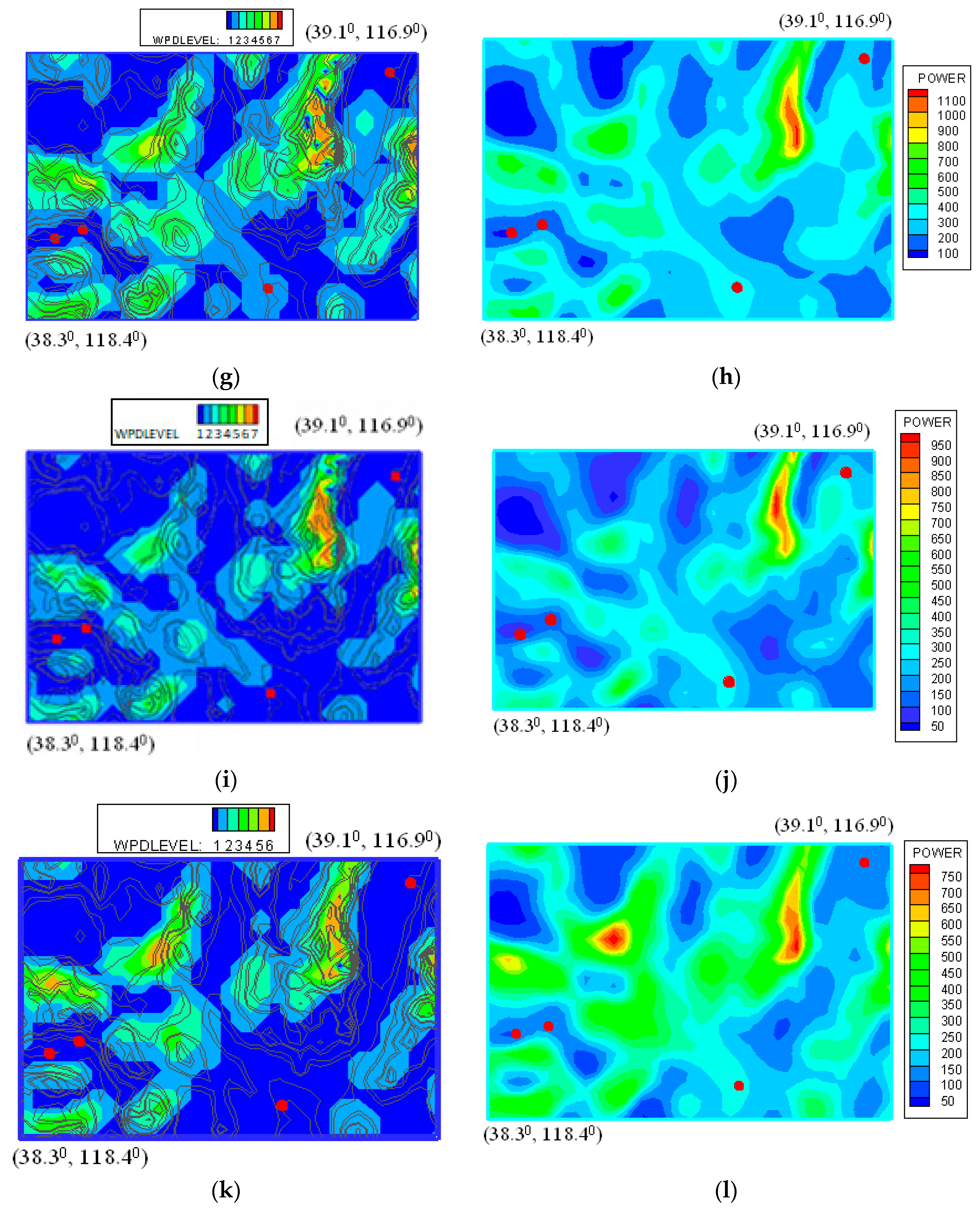
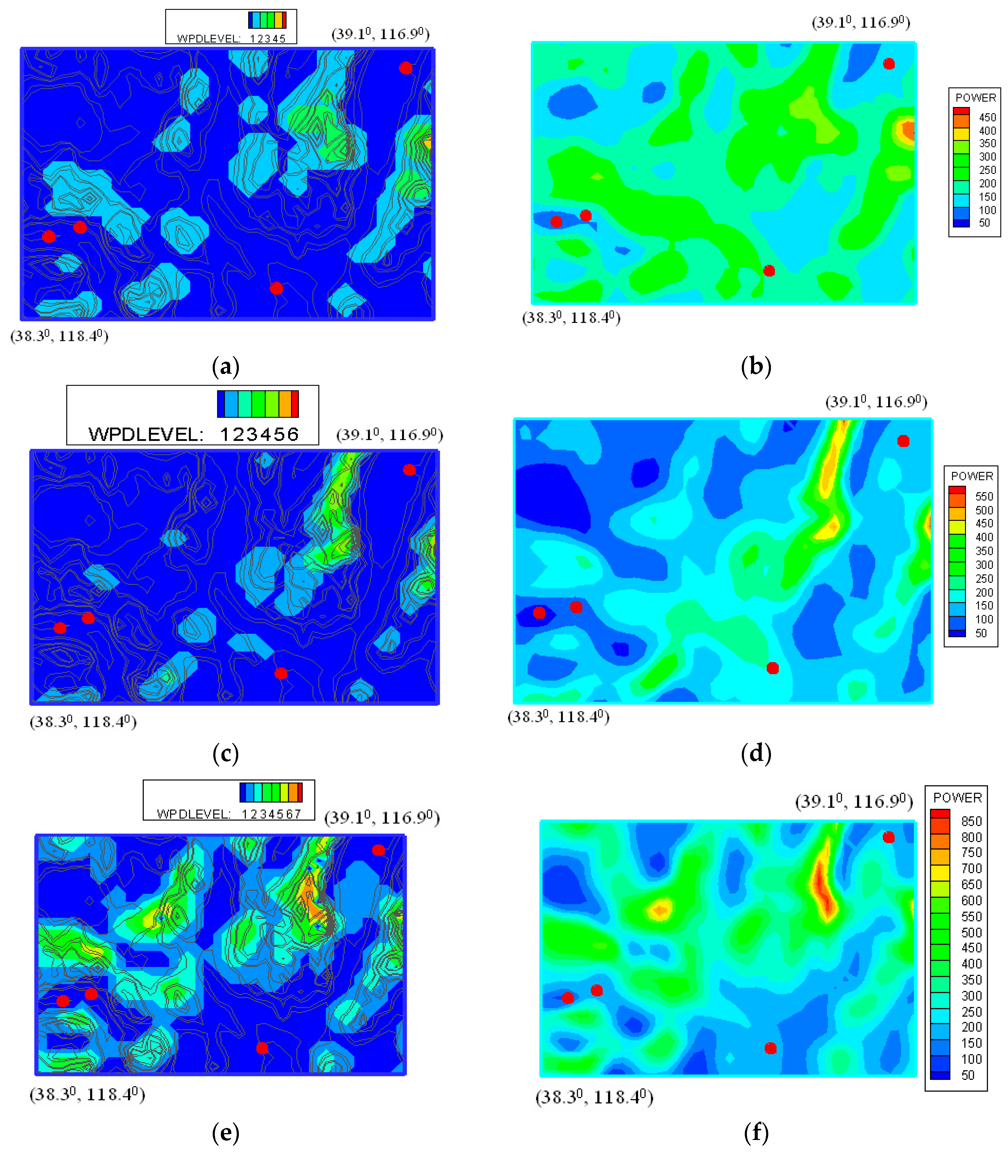
The resulting power density contours per month for September 2001 to February 2002 are shown in Figure 13a–l.

6. Implementation of the Meshless Method for Mobile Applications

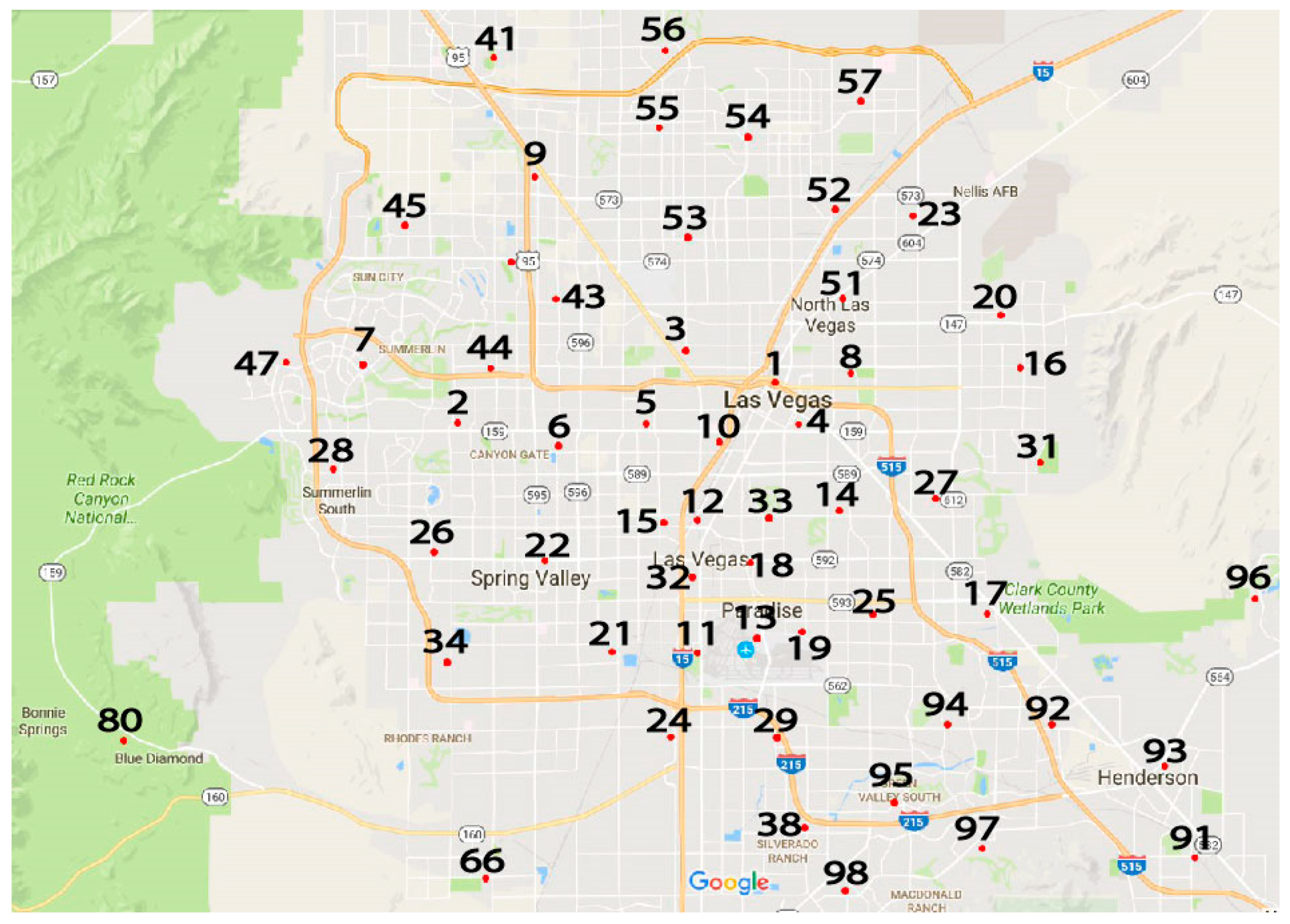
An advantage of the meshless method is its ability to run quickly and without the need for a supercomputer. This makes it an ideal method to run on a mobile application. A mobile application was developed to provide first responders with a 3-D wind field [27]. A local meshless technique obtains wind speeds, wind direction, and temperature data from various fire stations. The fire stations represent the nodes, which do not need to be meshed.

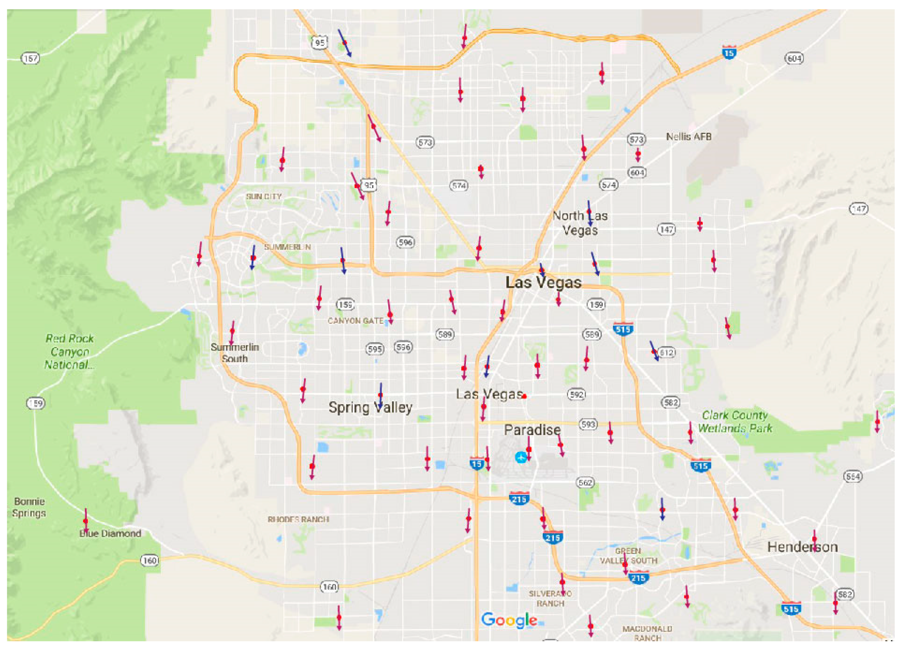
Figure 14 depicts fire stations across the Las Vegas Valley with their fire station numbers. Currently, the Clark County Department of Air Quality monitors resultant wind data in miles per hour and resultant wind direction measured in degrees compass. The monitoring stations information was used to collect initial wind speed and direction data closest to the fire stations. A hypothetical wind field was then developed showing information coming from each of the fire stations. Figure 15 illustrates the wind field.

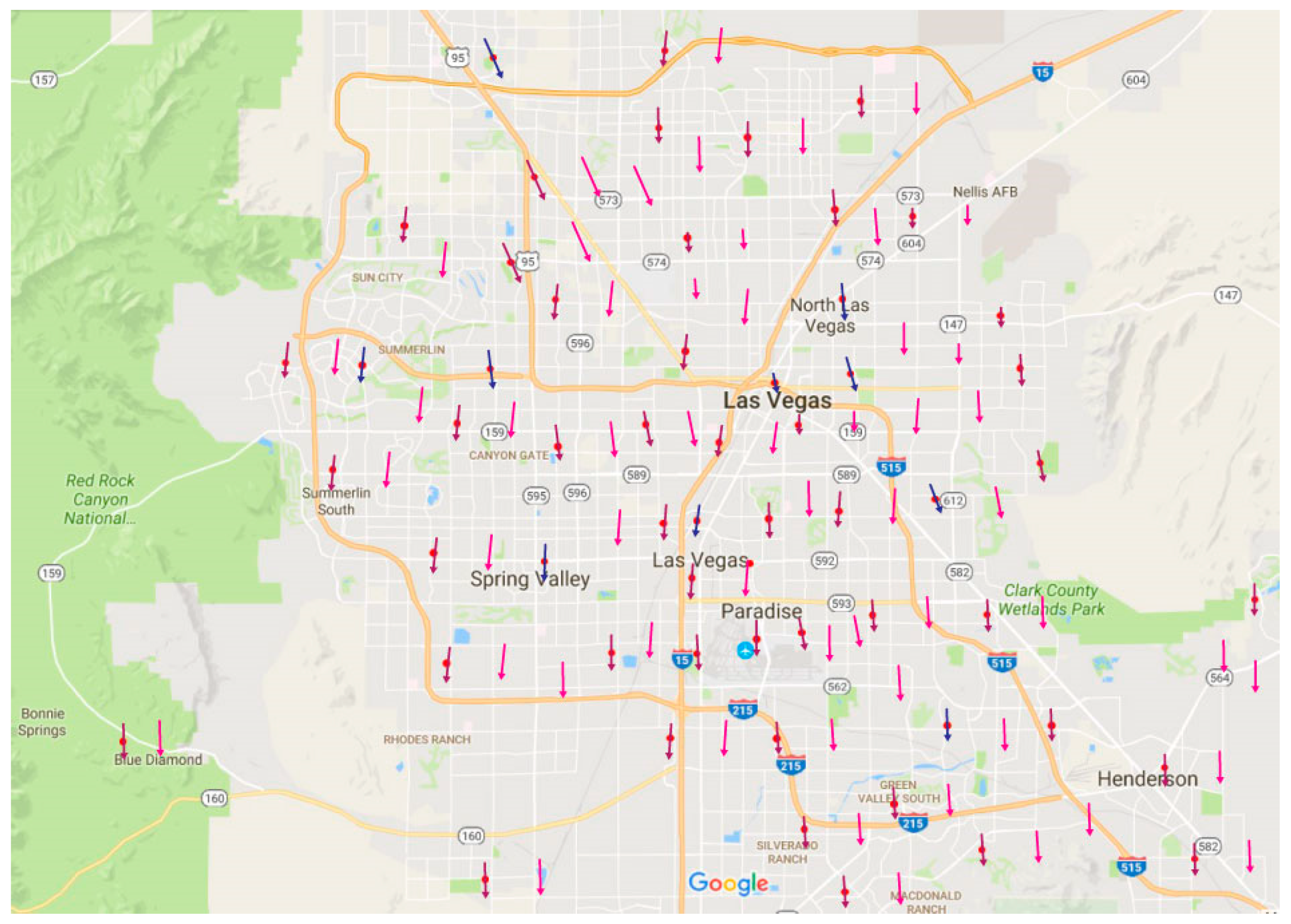
Currently, the Clark County Department of Air Quality monitoring stations provide data once an hour. The goal of the fire station monitoring stations would be to provide “real-time” updates. Depending on the equipment used, this can range from 10 min to as low as 1 min, depending on the accuracy of the data needed. The fire stations serve as the nodes for the meshless method. Once the intermediate wind vectors are populated, the updated image can be pushed to the mobile application. 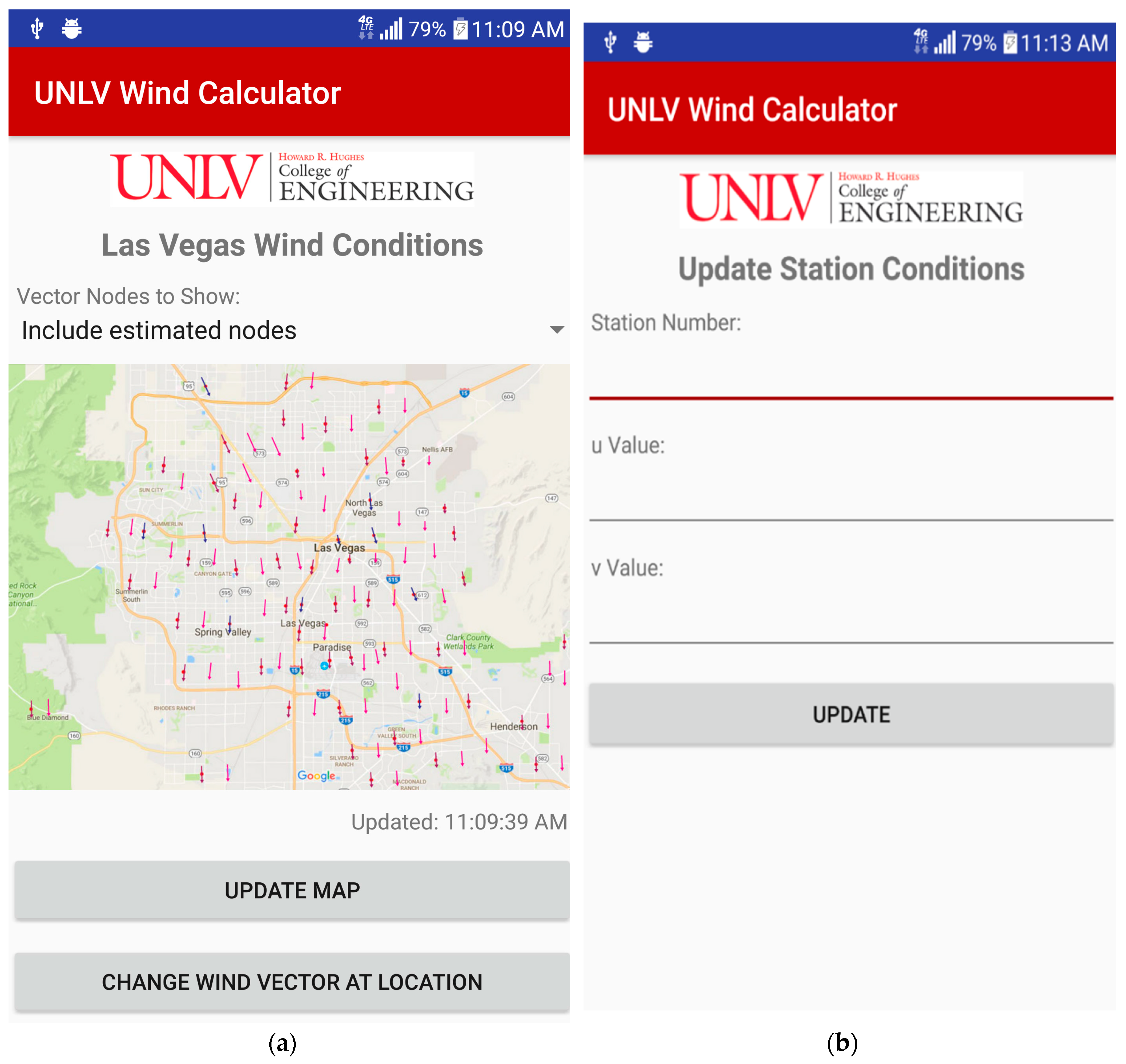Figure 16 illustrates the image a first responder would observe of a populated 3-D wind field on a mobile device (Android version).

An online connection is not always available for first responders in remote areas. The application can run independently of the server’s information. A first responder would have the ability to call into a fire station of choice, collect u and v values for the wind data, and input them into the mobile application. The application would then run the meshless algorithm and update the map independently of the server. Once connection was established again, the server would push the latest information to the mobile device. Figure 17a,b depict the layout of the application and the various output maps and data inputs.

First responders have the flexibility of choosing what type of map to view through a drop-down menu. Options include fire station numbers only, fire station vectors, and populated vectors. A button enables them to update the map whenever they want, otherwise, the map will update every time data is available when a wireless connection is established. If there is no connection and a first responder would like update a specific node, the “change wind vector at location” button leads to a menu where the fire station number and u, v wind speed values can be input. This proof-of-concept mobile application has great potential and will be available for users in the future.

7. Conclusions

A localized meshless method has been developed to calculate 3-D wind fields utilizing sparse data obtained from meteorological towers. Results were compared with field data obtained from a network of meteorological towers located at the Nevada Test Site (Nevada National Security Site) and an h-adaptive finite element model. The meshless method produced nearly identical wind velocity values and patterns as the h-adaptive finite element method, but with significantly less computational cost and difficulty.

The advantages of using localized meshless methods for meteorological simulations are significant when dealing with large, complex terrains, and completely eliminates the need for complicated and detailed meshes common to conventional numerical approaches. Additional node points can be easily added or removed from problem domains without having to re-mesh the entire system. The localized meshless technique is not only more computationally efficient but also yields equally accurate results compared with mesh-based methods. Current efforts are now underway to implement the method to display 3-D real-time wind data on mobile devices for use by the Las Vegas Fire Department in emergency response situations within the Las Vegas Valley.