A Mathematical Spline-Based Model of Cardiac Left Ventricle Anatomy and Morphology ^†

Abstract

Computer simulation of normal and diseased human heart activity requires a 3D anatomical model of the myocardium, including myofibers. For clinical applications, such a model has to be constructed based on routine methods of cardiac visualization, such as sonography. Symmetrical models are shown to be too rigid, so an analytical non-symmetrical model with enough flexibility is necessary. Based on previously-made anatomical models of the left ventricle, we propose a new, much more flexible spline-based analytical model. The model is fully described and verified against DT-MRI data. We show a way to construct it on the basis of sonography data. To use this model in further physiological simulations, we propose a numerical method to utilize finite differences in solving the reaction-diffusion problem together with an example of scroll wave dynamics simulation.

1. Introduction

Integrative mathematical models of complicated hierarchic physiological systems, such as the heart, allow the use of a computational mathematical approach to describe these systems from the molecular level to the macro level, which characterizes the structure and functions of the whole heart and/or certain heart chambers, including the LV. In the framework of numerical experiments, a comprehensive analysis of such ventricular models provides a way to elucidate the mechanisms of normal and pathological heart performance; these models also provide a way to predict potential methods of effective therapy, such as correcting mechanical and electrical cardiac function disturbances.

Preferential paths for the propagation of an electrical excitation wave in the human ventricular myocardium are associated with muscle fibers in tissue. The speed of an excitation wave along a fiber is several times higher than that across the direction of a fiber. Thus, 3D simulation of electrophysiological and mechanical activity of the heart requires an anatomical model that includes a field of myofiber directions.

Recently, several models of the electrical and/or mechanical activity of the whole heart or its chambers have been proposed [1,2,3,4,5,6,7,8,9,10,11,12]. The most valuable of these are based on a detailed description of cardiac anatomy and the fiber orientation field, which is crucial for a correct representation of the physiological function of the heart.

In the existing literature, there are two approaches for modeling heart chamber architectonics, including the morphological pattern of myocardium fiber orientation. The approaches are more complementary to each other than alternative ones. For convenience, we have roughly and non-rigorously assigned them as empirical and theoretical approaches.

In empirical approaches, fiber orientation is directly measured in the heart using various experimental techniques, and in theoretical approaches, fiber orientation is generated using algorithms.

1.1. Examination of Individual Hearts and Empirical Models

Important and useful empirical approaches are represented in several well-developed published models [13,14,15]. These models are based on the detailed experimental mapping of individual hearts. In current research, directions of fibers in the myocardium can be measured by different experimental methods. Particularly, the diffusion tensor imaging (DTI) technique has been used to obtain images that show the fiber orientation and anisotropy of the heart [16,17,18,19]. Such measurements can be done with a spatial resolution of up to 0.3–0.5 mm and, in general, produce high-quality data, which can be used in computer-based models.

Another way of measuring anisotropy directly is the tedious histological study of fiber direction in 3D [20,21], where the researcher makes a series of parallel slices of the part of the heart under investigation. In every slice, angles of the fiber slope are measured. When all of the angular values are composed, the researcher obtains a full picture of the fiber directions in the organ.

The initial quantitative approach to describing animal and human heart anatomy was established by Streeter in the 1960s [20]. It is worthy of note that all of the approaches on fiber orientation in the human heart are either based on or use the results of Streeter’s classical studies. Streeter not only measured fiber orientation in the heart, but also proposed several hypotheses on how this fiber orientation could be reproduced using geometrical transformations. However, for a long time, Streeter’s ideas were not implemented in a mathematical model.

The question of laminar arrangement in the muscular fibers and sheets is one of the basic matters in cardiac anatomy. Such an arrangement is hard to measure and is still under debate [21,22,23]. We have not attempted to include it in our present description.

Every directly-measured dataset is connected to one concrete patient or laboratory animal and, thus, cannot be directly used for personalized heart models. Hence, there is a demand for algorithms that will allow existing data to be projected onto any geometry (see [18]) or that will allow researchers to generate such fiber orientation fields from any given geometric data.

At the same time, strictly speaking, any model built on the basis of a particular arrow map is a model of one particular heart, as it is difficult to distinguish between the common properties of the heart of a given species and the individual specificity of the scanned heart sample. Of course, individual computational models of heart chamber architectonics built with the empirical approach may be developed further, up to the species model level. Correct averaging of data obtained via the mapping of individual heart samples will be necessary for this. Several promising works are focusing on this goal [24,25,26,27]. Models based on the empiric approach might, among other things, essentially contribute to the parameter verification of the models developed via the theoretical approach.

Each of the listed experimental methods allows researchers to obtain the fiber orientation field and use it to set up a model, and this approach is the best one to study a particular heart for which the measurements were performed. However, a researcher may not only need to study a given anisotropy, but also to modify it, e.g., to study its effects on various electromechanical processes. In many cases, anatomy alone, not fiber orientation, is known, and some algorithms are needed to build up the anisotropy. Such algorithms are based on generic views of cardiac anatomy, which have been obtained through more than a century of cardiac research.

1.2. Theoretical Models of Cardiac Anatomy

The theoretical approach to the modeling of heart chamber, e.g., the LV, architectonics arises from the attempt to clarify a general principle or governing rule that determines the orientation of the fibers in the ventricle wall. Such theoretical models may be especially useful when studying basic mechanisms of normal and pathologic heart performance.

The discovery of rotational anisotropy in the myocardium was one of the first fundamental findings in qualitative heart anatomy. The tangents to the myofibers turn, if we look at them transmurally, and the turning angle equals approximately 120°. Streeter compared this picture with a Japanese fan [20]. Torrent-Guasp suggested that we consider the myocardium of both ventricles as a “flattened rope” or a band that has two endings and makes a few turns [28]. According to Streeter [20], myofibers are geodesic lines on a set of nested toroids, and outer toroids are more prolate, while inner ones are more round. Besides this model, there are many models concerning a few myocardial layers (usually three, namely superficial, middle and deep; see, for example, [29]). One can find a more detailed description of the history of cardiac qualitative anatomy in [30].

One group of models constructs the architectonics of myocardial fibers by using the analogy of muscular skeletal fibers. Different models include from one to four systems of myocardial bundles [31,32,33,34,35]. However, some researchers point to restrictions of the approach [36,37,38].

Another hypothesis to LV architectonics considers it as a kind of vascular musculature, where many junctions between the fibers exist [39,40,41,42,43].

One of the key questions concerning the LV myocardium is related to its layers, namely their existence, and if they exist, their number and positions. As a rule, models with sheets have a number of layers inserted one into another [29]. Nevertheless, a layers-based model exists in which the number of sheets is indefinite and the LV is not divided into internal and external parts. The model in question is from an early work [28], published in 1973, in which Torrent-Guasp proposed a hypothesis on how cardiac fiber orientation could be reproduced using geometrical transformations. However, this idea has never been formulated in mathematical terms.

Let us now discuss mathematical models of the heart. Theoretical approaches to cardiac architectonics include rule-based methods [44,45,46] and the mapping of fibers from animal hearts to human heart geometry [47]. One of the most recent rule-based methods is a Laplace–Dirichlet algorithm [46], which takes a noisy DTI-derived fiber orientation field as input data and yields, firstly, the transmural and apicobasal directions for the entire myocardium and, secondly, a smooth and continuous fiber orientation field. Another approach was used by Peskin, who derived the fiber orientation field from the principles of mechanical equilibrium [48].

Chadwick considered a cylindrical LV model and specified the helix angle linearly depending on the position of the point in the LV wall [49]. A spheroidal LV model, which involved the linear dependence of the helix angle on the distance between the point and the endocardium, was proposed by Beyar et al. in [2].

Another theoretical approach was created by Arts et al. in 1992 [50]. Their model was an ellipsoidal LV with a piecewise quadratic law for helix angle change. The mechanical adaptational principle suggested by Arts et al. in 1982 [51] was used to quantify the orientation of muscle fibers via the helix fiber angle distribution.

1.3. Relation to Other Anatomical Ventricular Models

Torrent-Guasp in [28] suggested that the LV can be represented as a set of embedded surfaces, i.e., muscular layers, covered by curves representing the myofibers. This idea was illustrated using Pettigrew’s proposal [52] of these surfaces having the form of a planar semicircle with a number of curves drawn on the semicircle. The sheets thereafter were transformed into conical surfaces. Finally, the heart was considered as a family of such conical surfaces inserted into each other. It may be noted that Streeter mentioned the importance of these ideas, but did not formalize them.

The present work develops two analytical LV models based on Pettigrew’s anatomical concept. One of the models is axisymmetric [53]. The other model is built on power functions and is not symmetric [54]. Heart anatomy was described in these works using a family of inserted non-conical surfaces, which allowed us to represent the smooth geometry of the LV properly. A family of lines on these surfaces was used to represent cardiac fibers. The entire model was expressed in terms of analytical functions.

Our experience shows that in many situations, a well-fitting non-symmetric LV model cannot be made using the approach from [54]. We faced this when we tried to make “power-function” models using sonography and tomography data of human hearts. The limitation of the approach is that the LV model cannot fit shapes of some real hearts accurately enough.

The new model uses splines instead of power functions and, as we will show in this paper, is flexible enough to fit real medical visualization data. At the same time, the new model uses analytical calculations, so some of the derivatives necessary for solving reaction-diffusion systems can be found exactly. In the proposed model, both the anatomy and fiber direction field are defined analytically. We calculate fiber slope angles in a local coordinate system and compare them with in vitro experimental data on human hearts.

In the next section, we describe the details of our model construction. In Section 3 and Section 4, we compare its output with experimental measurements of anisotropy in the human and canine LV. In Section 5, we propose a technique for constructing a model based on sonography data, which is especially important for clinical applications. Section 6 and Section 7 provide a numerical method for simulating the electrophysiological activity of the LV and an example of the usage of the numerical method. Finally, Section 8 is a discussion on the results obtained.

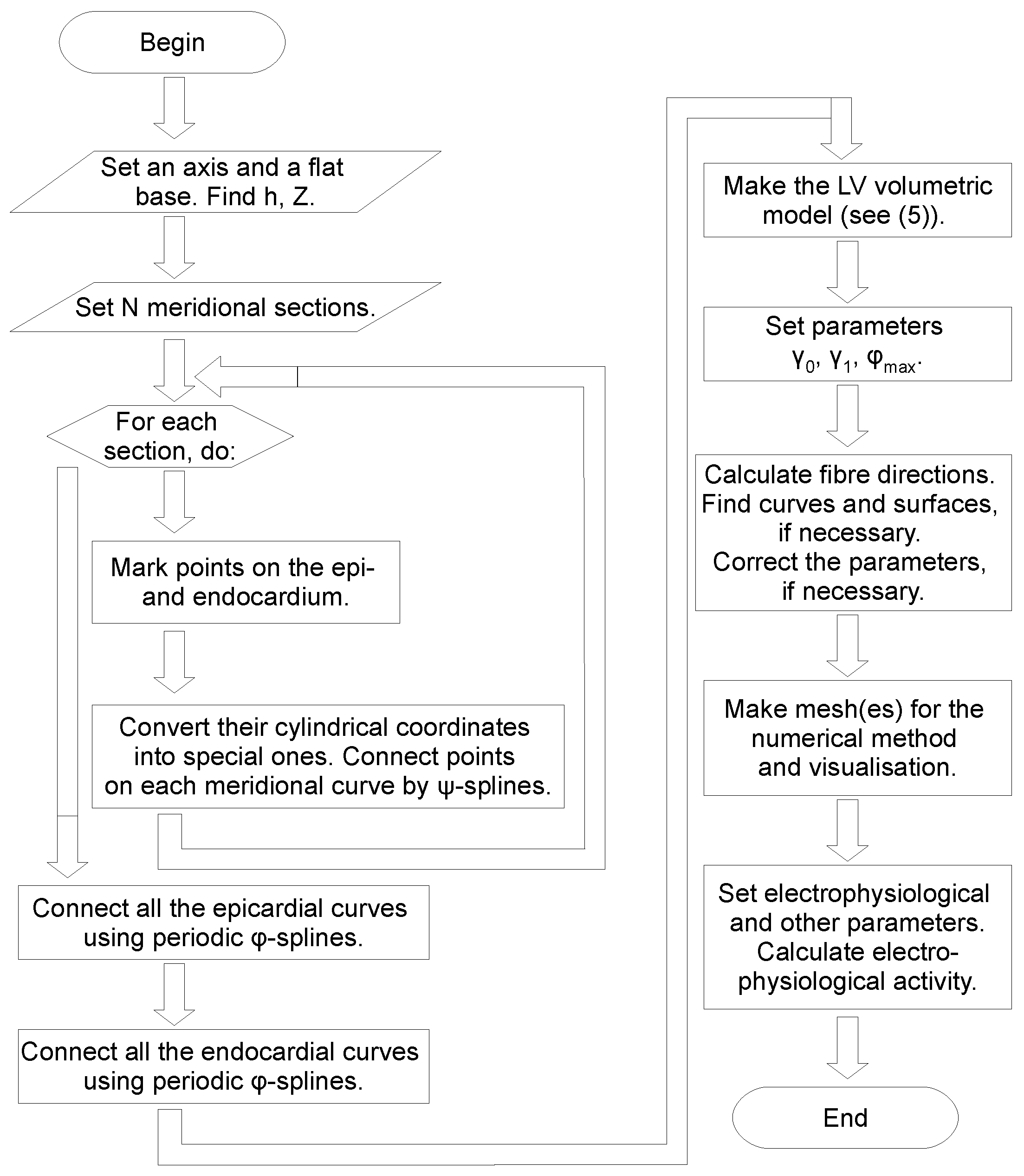
2. Construction of the LV Model

In order to define the LV form, we use a special coordinate system $(\gamma ,\psi ,\varphi ),$ where the variable $\gamma \in [0,1]$ corresponds to the position of a point in the LV wall layer: $\gamma =0$ is the endocardium; $\gamma =1$ is the epicardium; $\psi \in [0,\pi /2]$ is an analogue of latitude; $\psi =0$ is the upper plane part of the LV model (fibrous ring and valve zone); $\psi =\pi /2$ is the LV apex; and $\varphi \in [0,2\pi )$ is an analogue of longitude.

Initial data for the model construction are:

• meridians ${\varphi }_i$, $i=0,1,\dots n-1,$ where measurements are taken;
• coordinates ${\rho }_{i,j}^{epi}$, $z_{i,j}^{epi}$, $i=0,1,\dots n-1,$ $j=0,1,\dots n_i^{epi}-1,$ of marked points on the epicardium;
• coordinates ${\rho }_{i,j}^{endo}$, $z_{i,j}^{endo}$, $i=0,1,\dots n-1,$ $j=0,1,\dots n_i^{endo}-1,$ of marked points on the endocardium.

Now, we describe our algorithm to construct the LV model. First, for each meridian of the epicardium, we connect the marked points by an interpolation curve (Figure 1). We obtain a set of n curves in this step. Second, for each latitude ψ, we connect the n points on the curves by a closed interpolation curve. Algebraically, this means that we use a periodic spline. We obtain an epicardial surface in this step. Next, we do the same for the endocardium and, finally, we fill the space between the epi- and endocardium by a linear function of γ.

This schema can be formalized using the following equations. To transform the special coordinates into cylindrical ones $(\rho ,\varphi ,z)$, we use a simple formula for z-coordinate transformation:

$$z(\gamma ,\psi )=Z-(Z-h\gamma )sin\psi ,$$

(1)

where Z is the LV height and h is the LV wall thickness at the apex. Using this formula, we calculate ψ-coordinates of the marked points:

$$\psi (\gamma ,z)=arcsin\left(\frac{Z-z}{Z-h\gamma }\right).$$

(2)

As mentioned above, $\gamma =0$ on the epicardium, and $\gamma =1$ on the endocardium.

In each section ${\varphi }_i$ on the epicardium (endocardium), we make an epicardial (endocardial) curve:

$${\rho }^{epi}(\psi ,{\varphi }_i)=spline(\psi ;{\psi }_{i,j}^{epi}\mapsto {\rho }_{i,j}^{epi}),{\rho }^{endo}(\psi ,{\varphi }_i)=spline(\psi ;{\psi }_{i,j}^{endo}\mapsto {\rho }_{i,j}^{endo}).$$

(3)

Here, spline is a cubic spline with a zero second derivative at the endpoints. The notation $spline(x;x_i\mapsto y_i)$ means a spline constructed by two given arrays of data, $x_i$ as an argument and $y_i$ as a response variable. Then, we interpolate to obtain a surface between the curves:

$${\rho }^{epi}(\psi ,\varphi )=spline(\varphi ;{\varphi }_i\mapsto {\rho }^{epi}(\psi ,{\varphi }_i)),{\rho }^{endo}(\psi ,\varphi )=spline(\varphi ;{\varphi }_i\mapsto {\rho }^{endo}(\psi ,{\varphi }_i)).$$

(4)

Here, we use a periodic cubic spline. Finally, we fill the entire LV wall:

$$\rho (\gamma ,\psi ,\varphi )={\rho }^{epi}(\psi ,\varphi )(1-\gamma )+{\rho }^{endo}(\psi ,\varphi )\gamma .$$

(5)

Usually, if n meridional sections are considered, the angles between them are uniform, so ${\varphi }_i=i\pi /n$, $i=0,1,\dots n-1$.

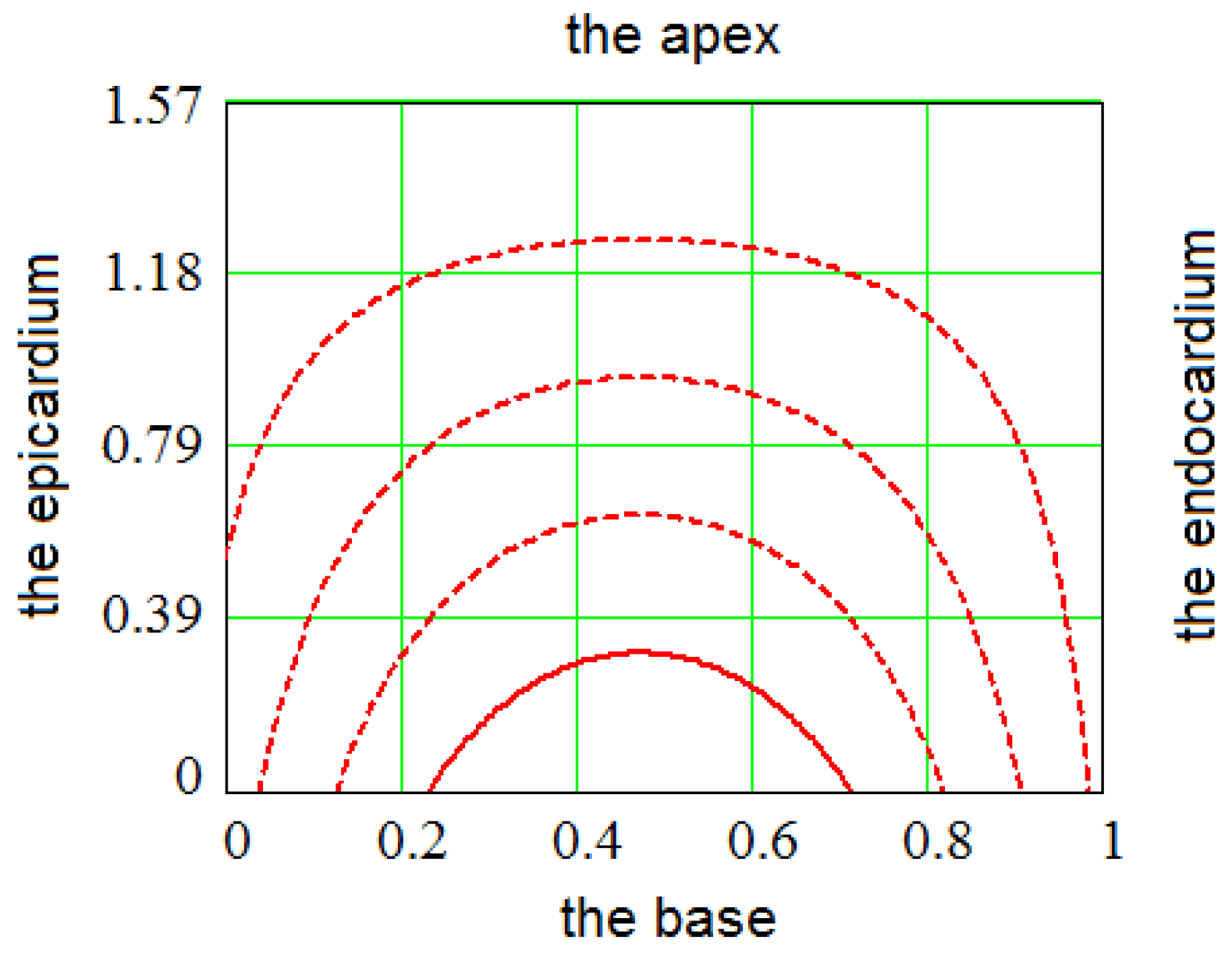
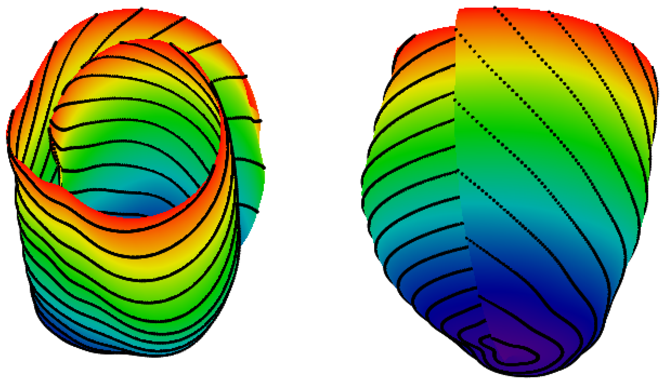
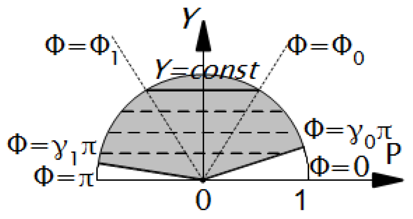
2.1. Spiral Surfaces

Hierarchically, the LV model is subdivided into muscle layers. In its turn, each layer is filled by myofibers. All of the layers have a spiral-like shape, so we call them “spiral surfaces” (SS). These surfaces have the same equation in special coordinates:

$$\varphi (\gamma ,{\varphi }_{min},{\varphi }_{max})={\varphi }_{min}+\gamma {\varphi }_{max},$$

(6)

where ${\varphi }_{max}$ is the SS twist angle (which is the same for all SS), and different values of ${\varphi }_{min}\in [0,2\pi )$ determine different surfaces. The equation of the SS in the cylindrical coordinates is shown below (see Equations (1) and (5)).

$${\rho }_{sp}(\psi ,\varphi ,{\varphi }_{min})=\rho \left(\frac{\varphi -{\varphi }_{min}}{{\varphi }_{max}},\psi ,\varphi \right);$$

(7)

$$z_{sp}(\psi ,\varphi ,{\varphi }_{min})=z\left(\frac{\varphi -{\varphi }_{min}}{{\varphi }_{max}},\psi \right).$$

(8)

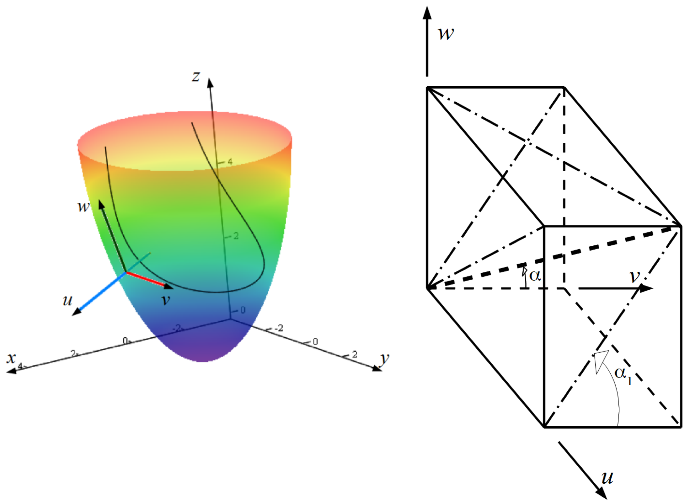
2.2. Filling a Spiral Surface with Fibers

We have utilized Pettigrew’s proposal [52] as we did in our previous models [53,54]. This proposal has been chosen because it can be formalized easily, and it describes both myofibers and sheets. Myocardial fibers are obtained as images of chords $Y=\mathrm{const},$ $Y\in [0,1)$ of sector $\mathrm{P}\le 1,$ $\mathrm{\Phi }\in [\pi {\gamma }_0,\pi {\gamma }_1]$ (the chords are parallel to the diameter $Y=0$) on the SS (Figure 2). Here, ${\gamma }_0$ and ${\gamma }_1$ $(0\le {\gamma }_0<{\gamma }_1\le 1)$ are parameters necessary to fit the sub-epicardial and sub-endocardial fiber angles. The parameter of any chord is the polar angle $\mathrm{\Phi }\in [{\mathrm{\Phi }}_0,{\mathrm{\Phi }}_1],$ where ${\mathrm{\Phi }}_0=max(arcsinY,\pi {\gamma }_0)$ and ${\mathrm{\Phi }}_1=min(\pi -arcsinY,\pi {\gamma }_1).$ The mapping of a chord point $(\mathrm{P},\mathrm{\Phi })$ to an SS point is defined by the formulae below (Figure 3):

$$\begin{array}{c}\gamma \left(\mathrm{\Phi }\right)=\frac{\mathrm{\Phi }-\pi {\gamma }_0}{\pi ({\gamma }_1-{\gamma }_0)},\\ \psi \left(\mathrm{P}\right)=(1-\mathrm{P})·\frac{\pi }{2}.\end{array}$$

For instance, if ${\gamma }_0=0$ and ${\gamma }_1=1$, the semicircle diameter is transformed into a fiber that begins on the basal epicardium, descends to the apex $(\mathrm{\Phi }=\pi /2),$ then ascends and ends on the basal endocardium. Images of shorter chords are located closer to the LV base and have shorter lengths.

An algorithm for calculating the fibre direction vector in points of the model is given in Appendix A.

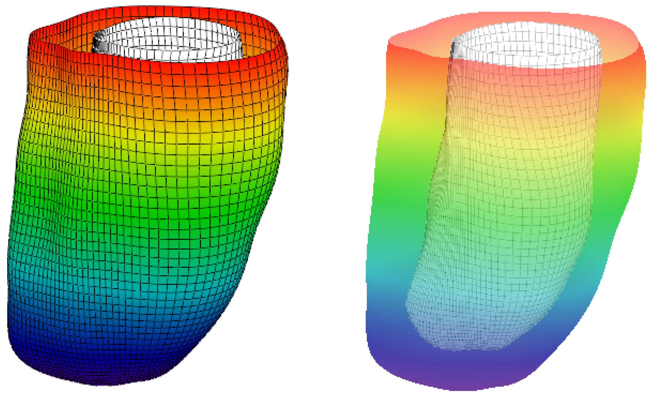
2.3. Fitting the LV Form

In [54], a fitting of the more rigid model to a real canine heart dataset was done with satisfactory results. Yet, fitting the dataset of a human heart into that model was less successful, partially due to the limitations of the model’s parameters. In this study, the same dataset of the human heart was used for the flexible model. The dataset is accessible online at [55].

The fitting procedure began with finding the LV axis $Oz$. Then, we sectioned the LV by $N=12$ meridional half-planes ${\varphi }_i=2\pi i/N,$ $i=0,1\dots N-1,$ passing this axis, and we manually marked points on the epi- and endocardium in each section. The mean numbers of points were 10 for the sub-endocardium and 11 for the sub-epicardium. In total, taking into account the coincidence of two apical points in all of the sections, there were 227 points. After setting the points, we used periodic cubic ϕ-splines and cubic ψ-splines. The results obtained are shown in Figure 4 and Figure 5.

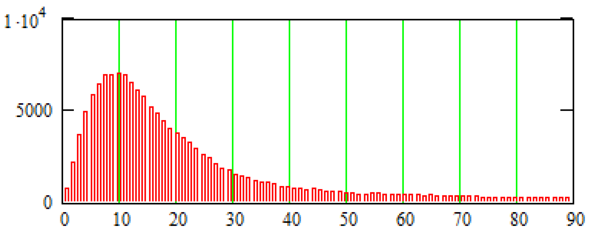
3. Methods for Model and Experimental Data Comparison

In the work [54], the theoretical model and experimental data were compared along normals to epicardial meridional sections as described in [20]. However, this method is not useful: normals do not have to intersect the endocardium, and they may intersect each other, so the task of finding a normal passing through a point may result in multiple solutions. In the present article, we use the special coordinates to construct straight pinning lines that do not intersect each other and always intersect the endocardium. These lines have a simple equation: $\psi =\mathrm{const},$ $\varphi =\mathrm{const}$.

We will now describe the comparison procedure. To compare angles along such a pinning line, one needs to specify a point A on the epicardium. Let its special coordinates be $\gamma =0,$ $\psi ={\psi }^{*}$ and $\varphi ={\varphi }^{*}.$ Let us consider a corresponding meridional section $\varphi ={\varphi }^{*}$ of the model, semi-plane Π. The line lies in Π and intersects the endocardium at a point B, having coordinates $\gamma =1,$ $\psi ={\psi }^{*}$ and $\varphi ={\varphi }^{*}.$ On the segment $AB,$ we set k equidistant points, including its ends, so that $A=A_1,$ $A_2,\dots ,$ $A_k=B$. The position of a point $A_i$ on the segment $AB$ is defined by the variable:

$${\mathrm{x}}_i=\frac{A_{i}B}{AB}$$

(for the endocardium $\mathrm{x}=0$; for the epicardium $\mathrm{x}=1$). We have to draw an SS through every point $A_i({\gamma }_i=(i-1)/(k-1),{\psi }^{*},{\varphi }^{*})$. The problem of finding such an SS is reduced to solving the SS Equation (6) with respect to ${\varphi }_{min}$:

$${\varphi }_{min}={\varphi }^{*}-{\gamma }_i{\varphi }_{max}.$$

Strictly speaking, there can be no points from the tomogram exactly on semi-plane Π; therefore, we selected points lying no further than $\Delta =1$ mm from the straight line $AB$ and inside the dihedral angle $|\varphi -{\varphi }^{*}|\le {\Delta }_{\varphi }=0.1$ rad $={5.7}^{\circ }$.

Streeter proposed specifying fiber direction using a local coordinate system $(u,v,w)$ and two angles, “true fiber angle” α and “helix angle” ${\alpha }_1$ [20] (p. 78) (see Figure 6); these angles are sufficient for specifying the direction of a fiber at a particular point. The true fiber angle reflects fiber direction totally, with both helix and transverse components, while the helix angle neglects the transverse part. The axis u is a normal to the epicardium pointed away from the LV; w is a meridian, i.e., an epicardial tangent lying in a meridional semi-plane and pointed upwards, and v is a parallel, i.e., vector $w\times u$. Angle $\alpha \in [0,\pi /2]$ is between a fiber and the parallel, and angle ${\alpha }_1\in [-\pi /2,\pi /2]$ is between the fiber projection on the plane $uv$ and the parallel.

We compared the two angular characteristics of fiber directions with the experimental data for a human heart in two meridians (one meridian lies in the LV free wall; another lies in the IVS) in the upper, middle and lower parts of the LV wall.

4. Results of Comparing the Model with DT-MRI Data

In this section, we compare the directions and angles of myocardial fibers in the model and DT-MRI data of one human and one canine heart.

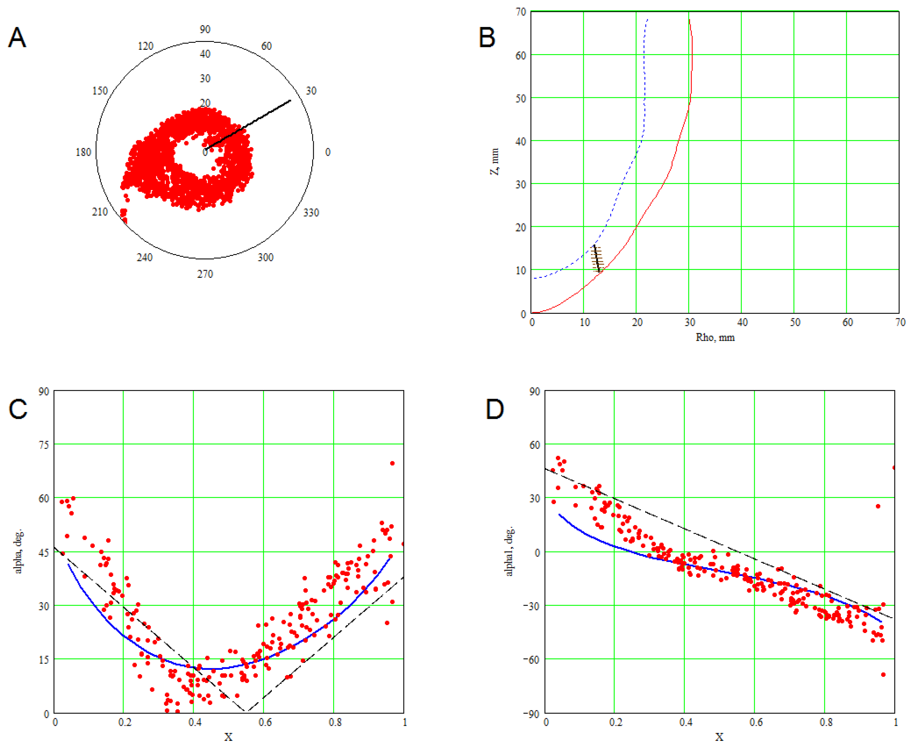
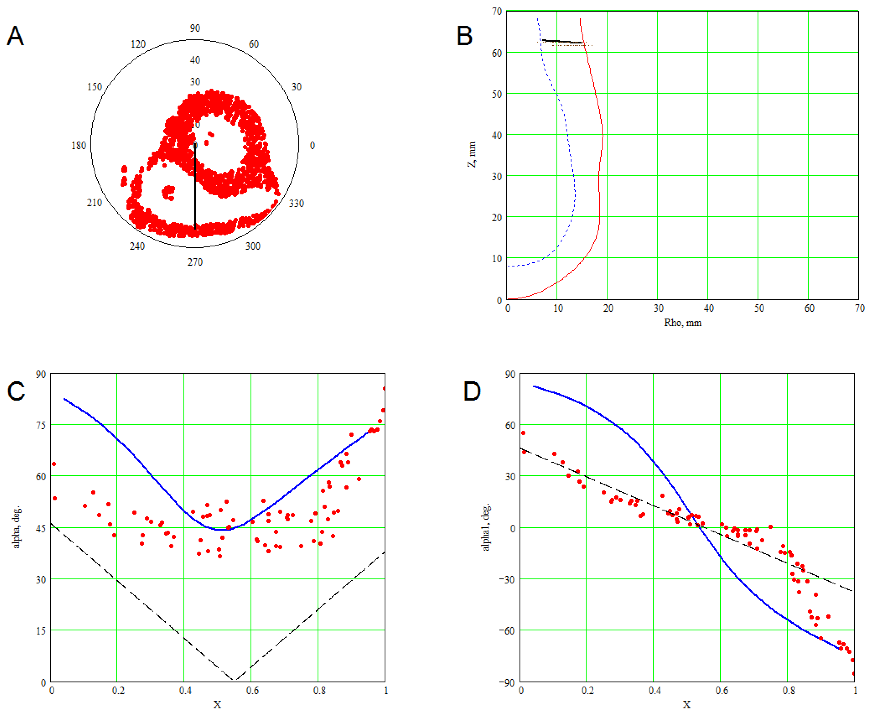
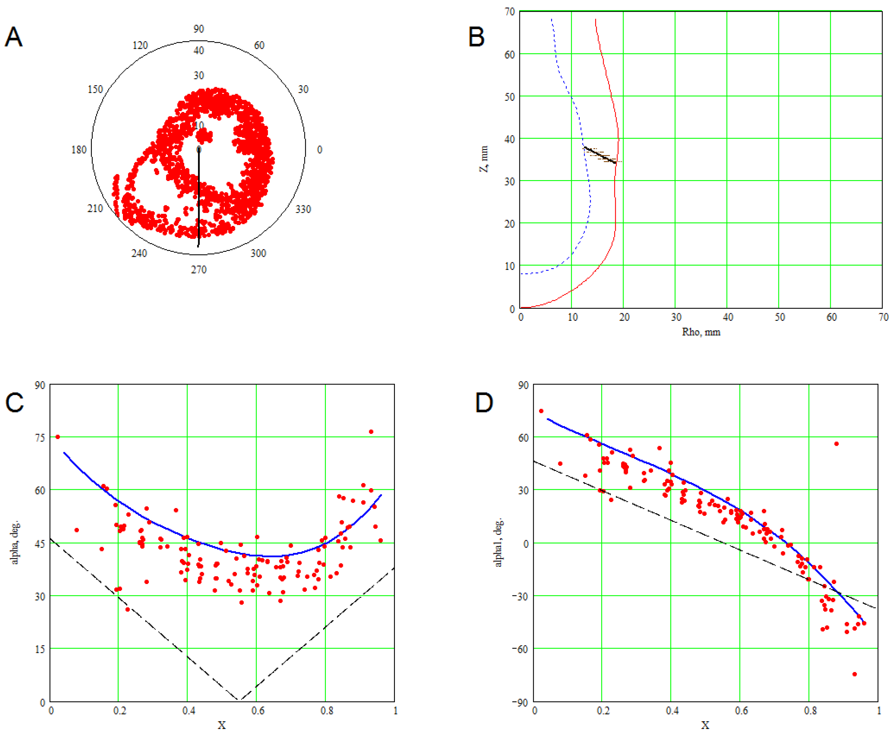
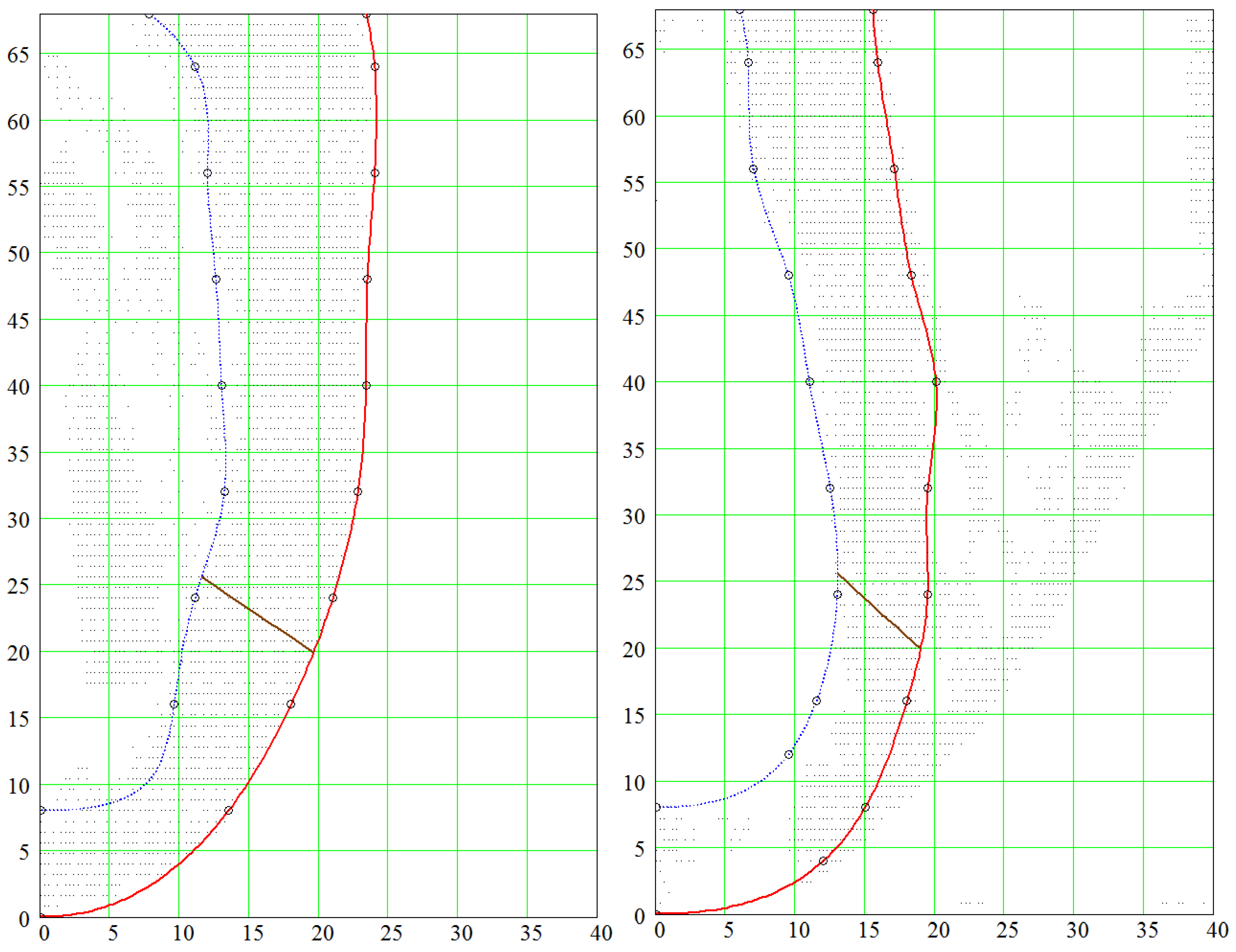
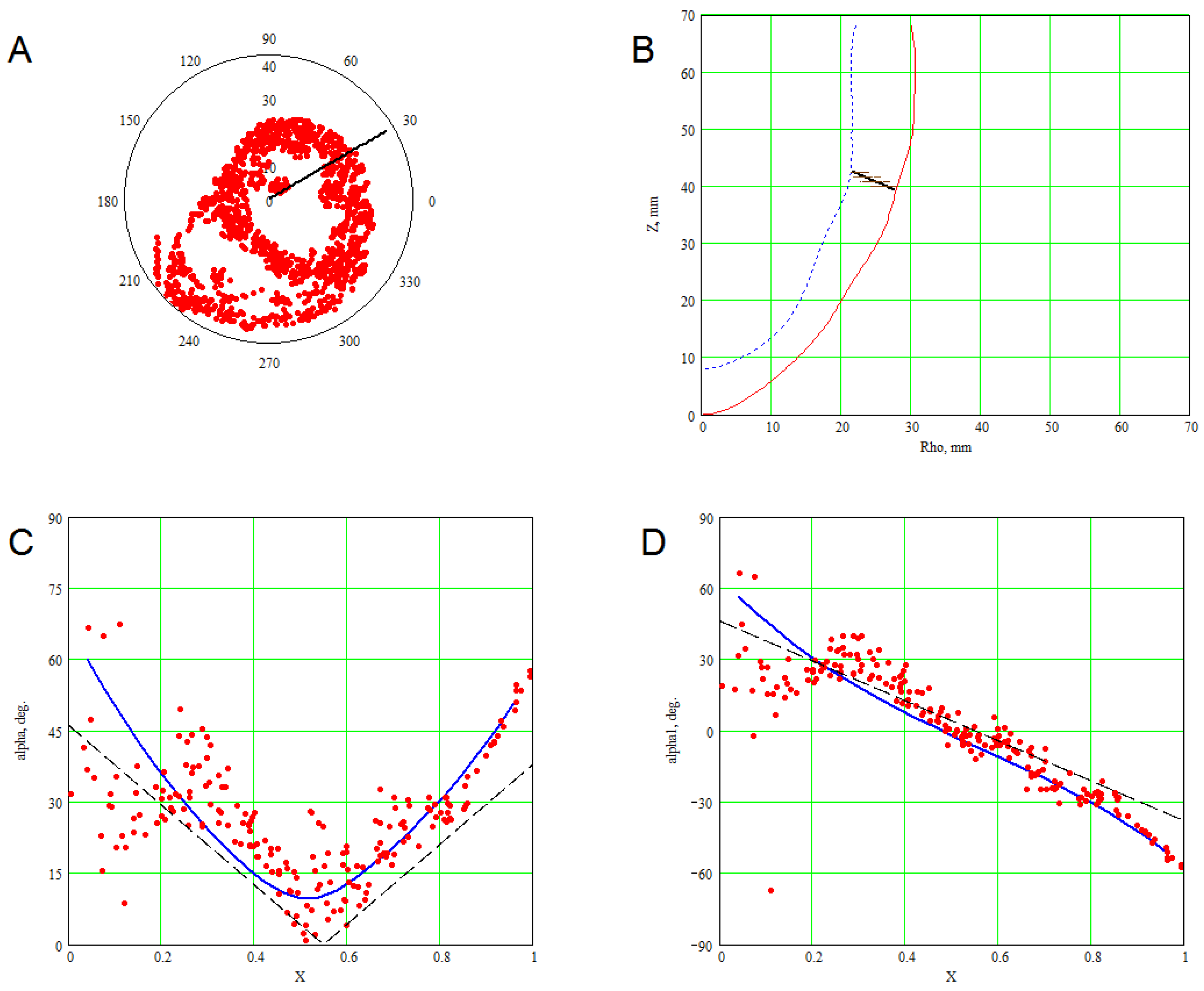
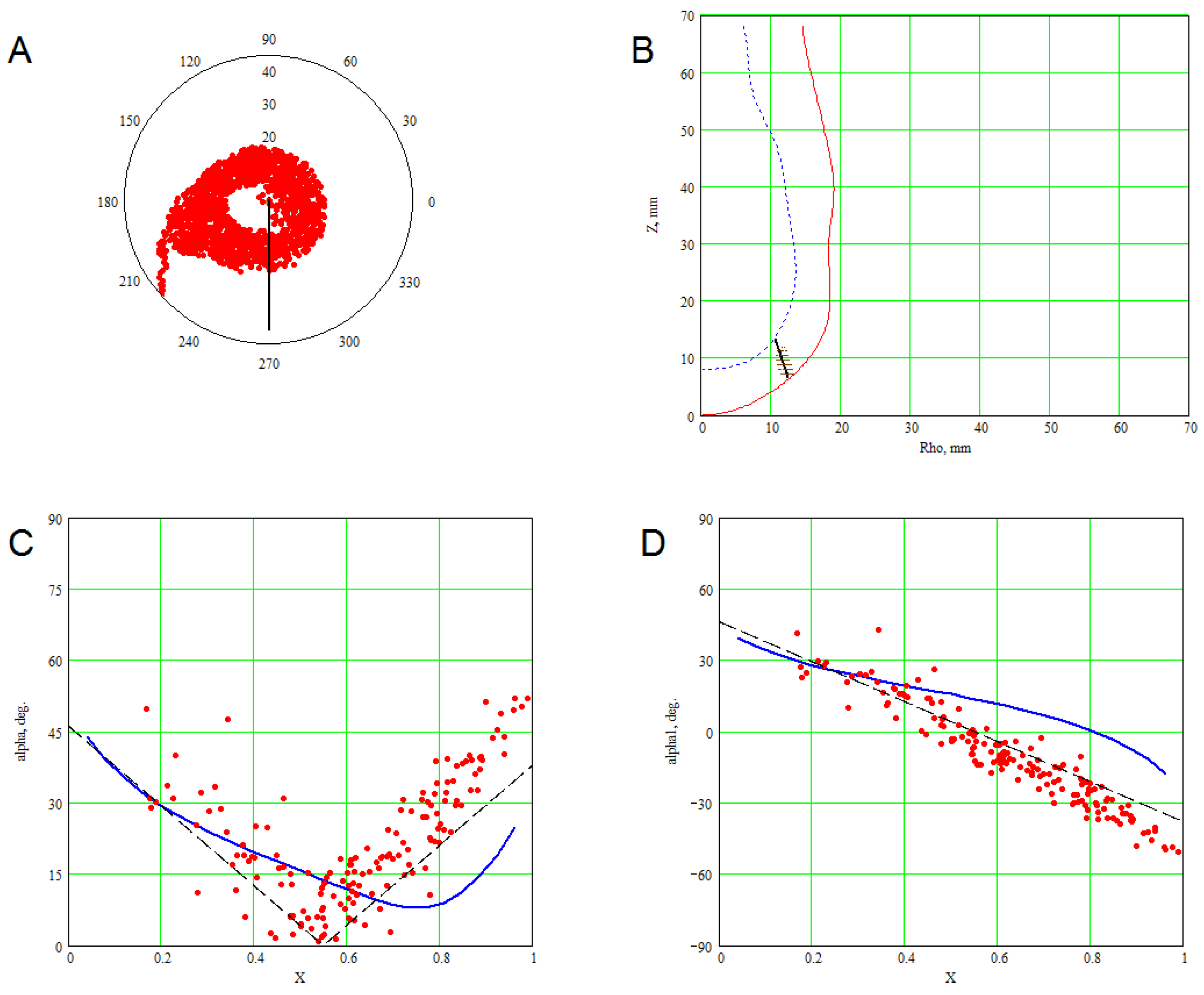
4.1. Comparison of the Model with Human Heart Data along Straight Pinning Lines

The following parameter values, which are common for all meridians, were used: LV height $Z=68$ mm, LV wall thickness at the apex $h=8$ mm, SS twisting angle ${\varphi }_{max}=3\pi$, endocardial fiber parameter ${\gamma }_0=0.13$ and epicardial fiber parameter ${\gamma }_1=0.9$.

Graphs of the dependency of angles $\alpha ,$ ${\alpha }_1$ on a point position on pinning lines are shown in Figure 7, Figure 8, Figure 9, Figure 10, Figure 11 and Figure 12. We will now analyze the results obtained.

At the upper and middle LV areas (e.g., Figure 7A and Figure 8A), one can see that the vertical axis does not go through the center of the horizontal LV sections, but it is situated closer to the IVS. The axis is positioned there because it must go through the apical LV area, and the LV apex projection to its basal plane is not situated at the center of the base. If one moves the axis to the base center, then the apex is far from the axis in one of the meridional sections; therefore, we cannot fit the LV wall shape using the central position of the axis.

Let us consider the fiber slope angles in one of the LV free-wall meridians. In the upper LV part (see Figure 7), the true fiber angle α (Panel C) in the model accurately reproduces the DT-MRI data. Angle α descends from 75° on the endocardium to approximately 15° at the middle of the wall, then it reaches 65° on the epicardium. The helix angle (Panel D) in the model is also quite close to the experimental data. The middle part of the free wall, which is determined by height (see Figure 8), shows an essentially large dispersion of the both angles’ values in the subendocardial zone $(\mathrm{x}<0.2)$. These angles’ values are similar to those in the basal zone, so the model can reproduce them well. The angles at the lower part of the LV free wall (see Figure 9) are predicted by the model with slightly lesser accuracy.

In the upper part of the IVS (see Figure 10), the model behaves in a different way than the experimental data. In the middle part of the IVS (see Figure 11), the model reproduces the angles reasonably accurately. Figure 12 shows that the model simulates the angles in the interior part of the myocardium better than in the exterior part.

The transmural variation of angle α is parabolic both in the DT-MRI data and in the model. This angle is locally maximal at the subendo- and subepicardium, and it is minimal, but not zero at the middle of the wall, where the helix angle is zero. Angle α is not zero there due to the traverse fiber angle.

The dashed black lines in Figure 7, Figure 8, Figure 9, Figure 10, Figure 11 and Figure 12 demonstrate the results of another modeling approach described in [46]. We see that the functions are linear with respect to $\mathrm{x}$, and the angles do not depend on the region. Bayer et al.’s model has zero transmural angle (traverse angle ${\alpha }_3$ in Streeter’s notation), so its angle $\alpha =|{\alpha }_1|$.

If one considers the fibers in the radial direction, our model (like the model from [53]) imitates the distinctive arrangement of fibers in the ventricular wall (see Figure 14 of [53]). As we mentioned above, this arrangement was called the “Japanese fan” by Streeter (see Figure 42C of [20]).

4.2. 3D Verification

We compared the fiber directions of the human tomography dataset and the model in all DT-MRI points located inside the model LV wall, and we made a histogram of the results (Figure 13). The mean angle between the two directions is 21.1°, and the median is 15.2°. The standard deviation is 18°.

Furthermore, we used our model to fit a canine DT-MRI dataset, which is accessible through the link [55] given in Section 2.3. The following parameter values, which are common for all meridians, were used: LV height $Z=90$ mm, LV wall thickness at the apex $h=12$ mm, SS twisting angle ${\varphi }_{max}=3\pi$, endocardial fiber parameter ${\gamma }_0=0.18$ and epicardial fiber parameter ${\gamma }_1=0.9$. A 3D comparison of the dataset and the model was performed. This comparison showed the following results: mean $19.5°$, median $16.1°$ and standard deviation $14.1°$, which is very close to the human heart comparison.

The degree of error in the angles consists of two parts. One of them is the modeling error caused by inaccuracies in the model. This error can be seen in Figure 7, Figure 8, Figure 9, Figure 10, Figure 11 and Figure 12, where the blue curves are out of the red point clouds. The second part is caused by errors of measurement and by the dispersion of data. Even if a blue curve is in the middle of a point cloud, such errors accrue. To identify these parts of errors, we partly averaged the true fiber angle $\left(\alpha \right)$ and helix angle $\left({\alpha }_1\right)$ data using the Smoothn function in MATLAB [56], so we obtained data without outliers. The averaging is controlled by the smoothing parameter $s\ge 0$. If $s=0$, the algorithm makes no changes in the input data. The noise in the data diminishes with the growth of s. Full averaging was impossible because an increase in the smoothing parameter above $s\approx 5$ led to an oversmoothing without an essential noise reduction. We used $s=5$, and the results of the 3D comparison are shown in

Table 1. Statistics of the error in the true fiber angle.

True Fiber	Canine		Human
Angle	Raw Data	Averaged	Raw Data	Averaged
mean	$12.3°$	$10.9°$	$12.5°$	$10.1°$
median	$9.2°$	$8.7°$	$8.8°$	$7.8°$
st. dev.	$10.8°$	$9.1°$	$12.2°$	$9.2°$

and

Table 2. Statistics of the error in the helix angle.

Helix	Canine		Human
Angle	Raw Data	Averaged	Raw Data	Averaged
mean	$15.2°$	$12.3°$	$18.9°$	$13.3°$
median	$11.0°$	$9.8°$	$12.1°$	$10.2°$
st. dev.	$16.5°$	$9.8°$	$22.6°$	$11.5°$

. There, “st. dev.” means “standard deviation”.

We can conclude that the partial averaging of the input data decreases the error sufficiently. The mean error in the fiber angles is about 10–15° for the data without outliers.

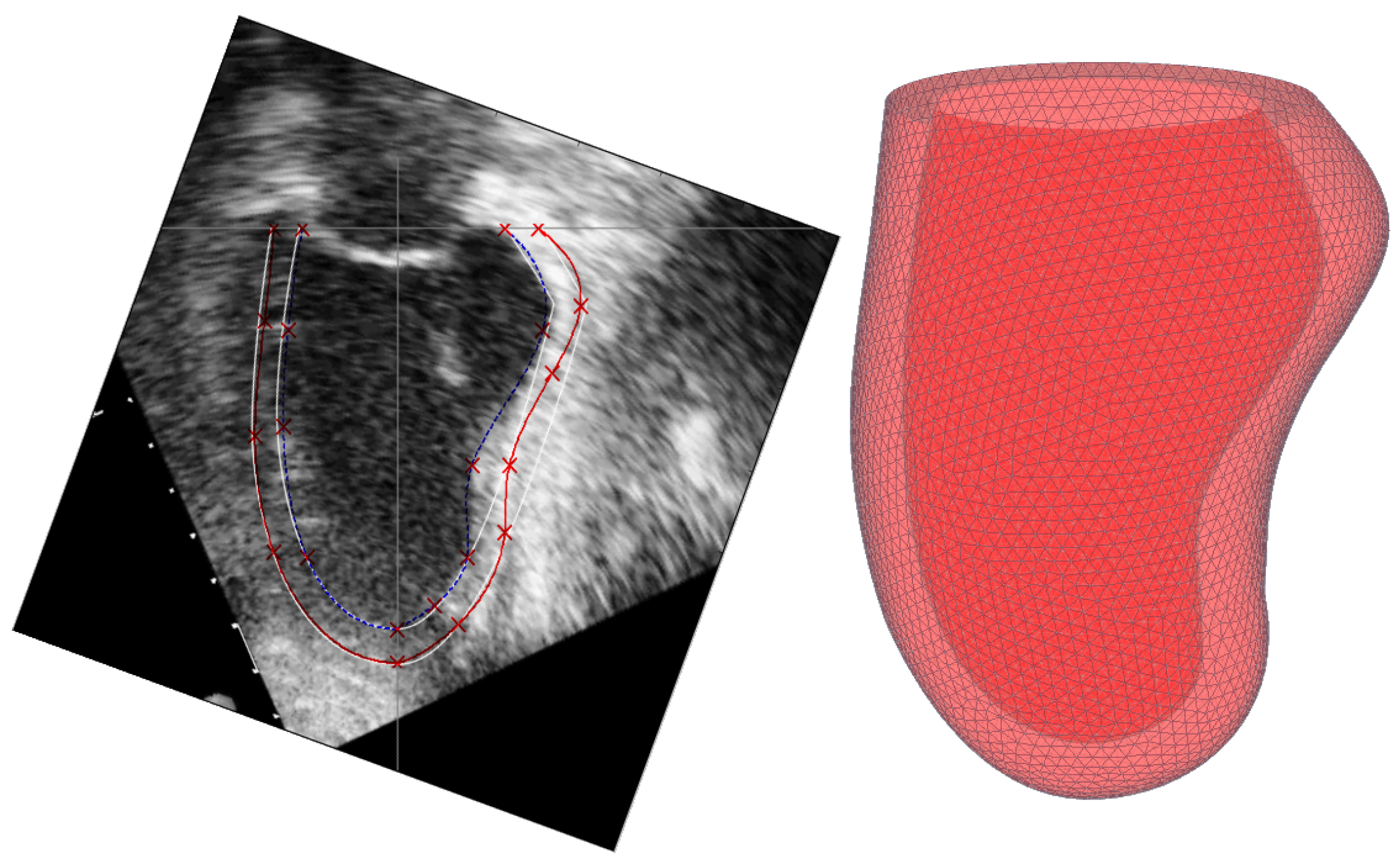
5. Constructing a Model Based on Sonography Data

The proposed model of the LV form can be constructed based on sonography data. We made one such measurement using data from two- and four-chamber views of one patient’s heart. In Figure 14, we show a comparison of two models: the old model based on power functions and the present spline-based one. The model was made using 44 marked points, from which 22 were endocardial and 22 were epicardial. Since the posterior (right on the image) part of the LV wall has a complex curved shape, it cannot be approximated accurately by the first model, but it can be well approximated by the second one. The anterior (left on the image) part of the LV wall has a simpler shape, so both models can be fitted into it well.

6. Numerical Method for Solving Reaction-Diffusion Systems on the Model

Electrophysiological processes in the myocardium are usually simulated using reaction-diffusion systems of partial differential equations. In the monodomain case, they are:

$$\begin{array}{cc}\hfill \dot{u}=& div(Dgradu)+f(u,\overrightarrow{v}),\hfill \end{array}$$

(9)

$$\begin{array}{cc}\hfill \dot{\overrightarrow{v}}=& \overrightarrow{g}(u,\overrightarrow{v}).\hfill \end{array}$$

(10)

Here, u is the transmembrane potential; $\overrightarrow{v}$ is the vector of other phase variables (its components differ in different models); the diffusion matrix D has elements $D_{ij}=D_2{\delta }^{ij}+(D_1-D_2)w_i(\overrightarrow{r})w_j(\overrightarrow{r})$, $i,j=1,2,3$; and $\overrightarrow{w}$ is the unit vector of the fiber direction.

The boundary condition of zero flux of the potential through the myocardial boundary looks like:

$$\overrightarrow{n}Dgradu=0,$$

(11)

where $\overrightarrow{n}$ is a normal vector to the boundary. In the case of complex cardial shape, implementation of the boundary condition is difficult, and it requires either a special method of Laplacian computation near the boundary in Cartesian coordinates or a special coordinate system where the boundaries are coordinate surfaces.

The LV base, epicardium and endocardium are just coordinate surfaces in the special coordinates linked with this model. Indeed, the base has the equation $\psi =0$, while the equation $\gamma =\mathrm{const}$ describes the epicardium and endocardium. For the symmetrical LV model, we proposed an algorithm [58], which has been used in a study of scroll wave dynamics [59]. For the previous (power-functions based) non-symmetrical model [54], a modified algorithm has been described elsewhere [60]. That algorithm can be used in the present case as well without any changes. However, since it was not published in English, we depict its dissimilarity with the symmetrical case method briefly here. Formulae for the Laplacian and boundary conditions in the special coordinates are given in Appendix B and Appendix C.

The Method to Rarefy the Computation Mesh

Let us consider a mesh node with indices $i,j,k$ of special coordinates $\gamma ,\psi ,\varphi$. In the case of the symmetric LV model, we propose that its γ- and ψ-neighbors have indices $i\pm 1$, $j\pm 1$. Its ϕ-neighbors have indices $k\pm Q\left[j\right]$, where Q is an array of natural numbers, and the differences are found so that the Cartesian distances between nodes are within some given limits. In the case of the non-symmetric LV model, we have to introduce six arrays instead of one, $Q_{var}^{dir}$, where $var\in \{\gamma ,\psi ,\varphi \},$ $dir\in \{+1,-1\}$. The meaning of $Q_{var}^{dir}$ is that the index of the γ-neighbor of the node in direction $dir$ is $i+dir·Q_{\gamma }^{dir}$. The index of the ψ-neighbor in direction $dir$ is $j+dir·Q_{\psi }^{dir}$. The index of the ϕ-neighbor in direction $dir$ is $k+dir·Q_{\varphi }^{dir}$. The values of Q have to be found once, at the initialization stage. If for a node $(i,j,k)$, at least one of $Q_{var}^{dir}\left[i\right]\left[j\right]\left[k\right]$ cannot be found, this node is marked “out-of-mesh”. We compute the potential in this node not by a finite difference method, but by interpolation, using the node’s closest “in-mesh” neighbors.

The flowchart in Figure 15 depicts all of the steps of construction and the use of the model in electrophysiological simulations.

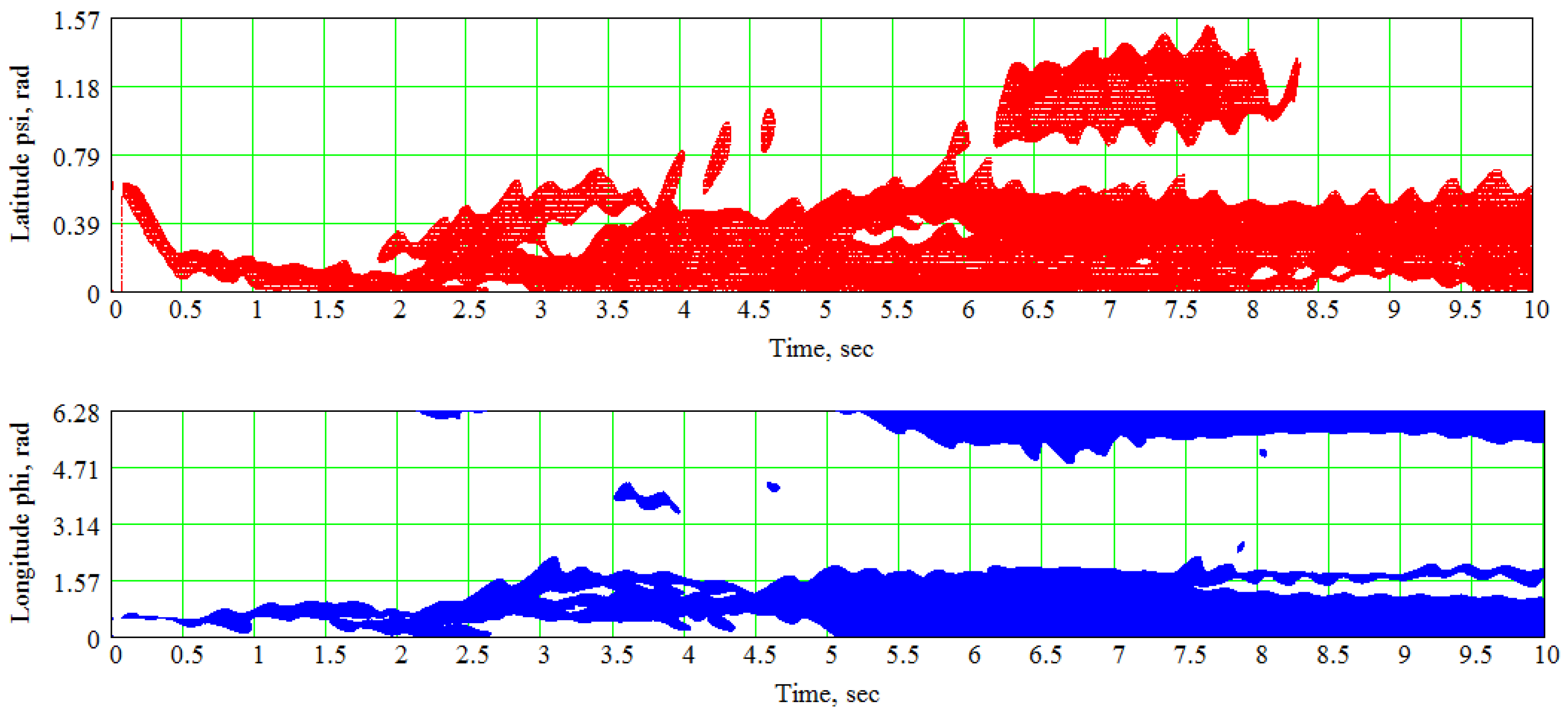
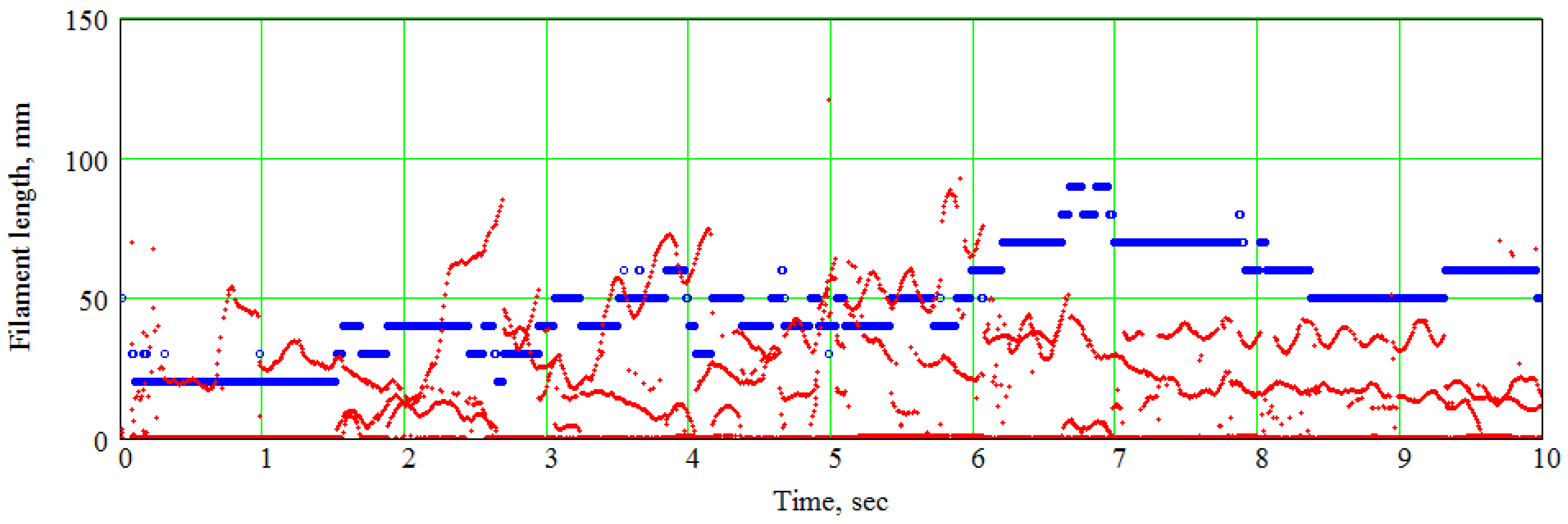
7. An Example of the Spline-Based Model’s Practical Usage in Electrophysiological Simulations

The model was used to study the dynamics of scroll waves of electrical excitation. Such waves are solutions of classical reaction-diffusion systems, and they correspond to dangerous arrhythmias, such as paroxysmal ventricular tachycardia and ventricular fibrillation. Our simulation was based on the Aliev–Panfilov model [61] of electrical excitation in the myocardium and the aforementioned human heart DT-MRI dataset and anatomical model (see Section 2.3 and Section 4). The electrophysiological model is dimensionless and has the following form:

$$\begin{array}{c}\frac{\partial u}{\partial t}=div(Dgradu)-ku(u-a)(u-1)-uv,\hfill \\ \frac{\partial v}{\partial t}=ϵ(u,v)(-v-ku(u-a-1)),\hfill \\ ϵ(u,v)={ϵ}_0+\frac{{\mu }_{1}v}{u+{\mu }_2},\hfill \end{array}$$

(12)

where u is the transmembrane potential, v is the conductivity for the K current in the membrane, $D_{1,2}$ are diffusion coefficients along and across fibers and k, a, ${ϵ}_0$, ${\mu }_1$, ${\mu }_2$ are cell model parameters. These parameters had the values $D_1=7.12{\mathrm{mm}}^2/\mathrm{ms}$, $D_2=D_1/9$, $k=8$, $a=0.1$, ${ϵ}_0=0.01$, ${\mu }_1=0.12$, ${\mu }_2=0.3$. A boundary condition provided zero flux through the LV boundary. Initial conditions were $u=1$, $v=0$ (initial stimulation) at $\psi \le 0.4·\pi /2$, $0\le \varphi \le 2\pi /12$; $u=0$, $v=k$ (initial temporary block of propagation) at $\psi \le 0.4·\pi /2$, $2\pi /12\le \varphi \le 2\pi /6$; and $u=0$, $v=0$ (resting state) elsewhere.

We used the spatial mesh size $dr=0.5\mathrm{mm}$; the time step $dt=0.01\mathrm{ms}$; and the dimension coefficients $5.4\mathrm{ms}$, as the model time unit, and $6.2\mathrm{mm}$, as the model length unit, based on the period and wavelength of a spiral wave simulated on a flat isotropic surface. The duration of the simulation was 10 s.

The results we obtained are shown in Figure 16 and Figure 17. From these results, we can see that the solitary filament drifted towards the base $(\psi =0)$, and then, several filaments appeared. The number of filaments slowly increased from 1 to 9 and then decreased to 5–6. This observation means that a tachycardia paroxysm transformed into a fibrillation.

8. Discussion

This section analyses the algorithm, compares it with other models and techniques, examines its methods of verification and concerns the usage and further development of the constructed model.

8.1. Advantages and Disadvantages of the Proposed Model

The model adequately reproduces the fiber angles in the LV free wall and in the middle zone of the IVS of the human heart. Nevertheless, the data agreement in the apical zone of the IVS is only qualitative; in the IVS upper part of the human heart, the model yields results that differ from the experimental data.

Our model has the following merits:

• It has relatively few parameters for shape, fibers and sheets.
• The LV apex is smooth thanks to the special choice of function z. This is a useful feature for integration methods sensitive to the smoothness of the boundary.
• It uses only simple one-variable splines, and no two- or three-parametric splines are required.
• The fitting of shape and fiber directions are independent tasks in this model.
• It is flexible enough to fit not only normal, but pathological LVs.
• It yields not only fibers, but also sheets.

Limitations of the model include the following:

• Similar to our previous models, its base is flat, which is not the case in real mammal anatomy.
• The fibers are not geodesic lines in the model sheets. It is difficult to determine if this is a disadvantage of the fibers, the sheets or both.
• Model fibers end at the base. However, this demerit can be amended by combining this model with the toroids-based one described in [62].
• It is unclear whether the model is generalizable for both ventricles.

8.2. The Present Model Compared with Other Qualitative Models

The ventricular myocardium’s structure and its qualitative description have been explored for several centuries. Reviews of experimental findings and theoretical conceptions can be found, for example in [23,63] and other reviews in the supplementary volume [64]. The present model is conceptually close to Krehl’s nested toroids to the extent that the LV myocardium, except the papillary muscles, is filled by non-overlapping surfaces, and each surface is filled by non-overlapping curves. The distinctive feature of the proposed model is the spiral shape of the surfaces. Whether the SSs are close enough to real heart sheets is a topic for future research.

In [20], Streeter proposed the geodesic principle of winding fibers on the sheets. This principle holds in the toroidal model, but not in the present one. However, if we keep the fibers only, the surfaces may be adjusted to them. This interesting problem remains for future research: How should we draw a set of non-overlapping surfaces on the given set of curves so that the curves are geodesic on the surfaces?

Some qualitative models of the myocardium describe its structure on the levels of cells, myofibers and myolaminae (see, for example, [22,29,65]); such models examine the interconnections and arrangement of cardiomyocytes and other types of cardiac cells. However, the main task of our model is to yield fiber and sheet normal directions in all points of the LV myocardium, but not to represent the amazingly complex micro- and macro-structure of the cardiac muscle. A union of our model with a structural tissue-level model, which includes Y-junctions of the cells, capillaries, fibrous tissue and other elements, would be of great practical value.

A key feature of the proposed model is its numerical, quantitative nature, so it should be compared with other quantitative models and data.

8.3. Comparison with Experimental Data and Quantitative Models

Some experimental techniques that can be used to verify our model have been mentioned in our previous work [54]. These techniques include DT-MRI (already used here), as well as micro-CT [66], histological investigation [67] and quantitative polarized light microscopy [30]. These methods provide fiber orientation data that may be used for the construction of anatomical computational models in different ways.

• Finite-element models can utilize the data as a discrete dataset [13,68,69].
• Rule-based models, i.e., the models formed on the basis of some constitutive rule [44,45,46,47], can be compared against the data, which allows them to be verified.

A comparison with a recent rule-based method, the Laplace–Dirichlet algorithm [46], and with a wrapping-based myocardium model [70] was done in our previous paper [54]. The idea of using splines to fit cardiac imaging data is not new. An example of such LV shape model, constructed with B-splines, together with a review of spline-based models, can be found in [71]. A common weak point of many such models, however, is a lack of computing fiber direction field.

A quantitative comparison with a model from [46] can be made by measuring the mean difference angle between the experimental and model data. Bayer et al. in [46] report that their result is $23°\pm 20°$. Our result on the human heart dataset is $21°\pm 18°$, and on the canine dataset, it is $19.5°\pm 14.1°$, which is comparable with their achievement.

Our model fits the shape of the LV and has only three parameters (${\gamma }_0$, ${\gamma }_1$, ${\varphi }_{max}$) to adapt fiber directions. Fiber directions can also be fitted through widely-used fitting functions with many more parameters, as was done in [72]. In that work, fiber direction field in mice was approximated in spheroidal coordinates by a product of two algebraic and one trigonometric polynomials. A certain advantage of that approach is its flexibility. The reported root-mean-square error was about $2.3°$–10°. Yet, that method usually requires about 10 parameters for each algebraic and 10–40 for trigonometric polynomials, whereas our technique uses only three parameters. Furthermore, the parameters in [72] have unclear geometrical or physical meaning, unlike ours. Moreover, the numbers of those parameters for different hearts vary, so the coefficients cannot be averaged to obtain recommended species-level parameter sets. We hope that our parameters can be averaged or fitted on the species level or at least for the norm and pathologies of particular species. This will allow researchers to construct fiber direction fields based on the shape of patients’ hearts without DT-MRI data.

Let us discuss the level of model error in the fiber directions. How can local and global cardiac characteristics be affected if the fiber angles change?

In an article by Campbell et al. [73], the electromechanics of dogs’ hearts was modeled using different cell- and tissue-level parameter values. One of the authors’ simulations included three models with different values of the total transmural fiber angle ${\alpha }_1$, i.e., 112°, 145° and 170°, while all other parameters were the same. The mean transmural difference of the helix angle between the middle model and the extreme models was about 12°. The authors discovered that such a fiber angle distribution affects the range of fiber strains and weakly changes hemodynamics and transmural delay in activation.

In a conference work by Wong et al. [74], the sensitivity of the average displacement of some points of the heart to epi- and endocardial fiber angles was studied. The angles were changed at increments of 20° from 20°–80°. The analysis showed that a minimal change of the angle (though 20° is an essential angle) leads to a significant variation in the displacement of the points. Our model has special parameters for fitting the epi- and endocardial fiber angles, so such a significant average error in these angles is unlikely to appear.

In Sánchez’s PhD thesis [75], linear and cubic laws of the helix fiber angle dependence on wall position were used in electromechanical simulations. The maximal difference between the angles was 23°, and it led to significant changes in maximal contraction time and total activation time.

Baron et al.’s conference paper [76] is focused on the effect of fiber orientation on LV stroke volume. A change of 10° in epi- and endocardial helix angles leads to the following effects: an 18% difference in the atrioventricular plane displacement, quite a small difference ($\approx 2$ mm Hg) in blood pressure in the LV, a 5% difference in the minimal LV-cavity volume, a 3.5% difference in the ejection fraction and a 2% difference in pressure-volume work.

Summarizing all of the aforementioned works, we conclude that fiber (helix) angle differences or errors on the order of 10° can sufficiently change the local parameters of cardiac activity, but affect its global characteristics lightly.

The goal of our model is to predict the average field of fiber directions for a given species. Therefore, the model error has to lie in the intraspecies limits. For example, the limits reported in [73] for dogs $(12°)$ are close to the error achieved by our model ($10.9°$; see Table 1), which justifies the relevance of our technique.

8.4. Further Development and Usage of the Model

The model does not include the uppermost part of the ventricular myocardium, the basal ring, where myofibers form torus-like shapes (Figure 14 of [28]). Moreover, some of the data available on the apical region show that myofibers there make toroidal layers, similar to basal ones (Figure 6 of [28]).

This model has been constructed based on and verified against only two DT-MRI datasets, one canine and one human. Such validation is limited, so its development is an important topic of our future research.

The spline apparatus enables researchers to use this model in cases of complex wall geometry, such as in patients with old myocardial infarctions, and other situations where the wall has loci of thickening and thinning.

The analytical description of cardiac geometry has been used in developing a new numerical method for the study of the electrophysiological activity of the LV. The model can also be utilized to generate different anisotropic properties of the heart, to alter the LV shape (by changing the model parameters) and to study their influence on cardiac electrical and mechanical functions.

References

1. Trayanova, N.; Constantino, J.; Gurev, V. Electromechanical models of the ventricles. Am. J. Physiol. Heart Circ. Physiol. 2011, 301, H279–H286. [Google Scholar] [CrossRef] [PubMed]
2. Beyar, R.; Sideman, S. A computer study of the left ventricular performance based on fiber structure, sarcomere dynamics, and transmural electrical propagation velocity. Circ. Res. 1984, 55, 358–375. [Google Scholar] [CrossRef] [PubMed]
3. Greenstein, J.; Winslow, R. Integrative systems models of cardiac excitation-contraction coupling. Circ. Res. 2011, 108, 70–84. [Google Scholar] [CrossRef] [PubMed]
4. Hunter, P.; McCulloch, A.; Keurs, H.T. Modelling the mechanical properties of cardiac muscle. Prog. Biophys. Mol. Biol. 1998, 69, 289–331. [Google Scholar] [CrossRef]
5. Tusscher, K.T.; Noble, D.; Noble, P.; Panfilov, A. A model for human ventricular tissue. Am. J. Physiol. Heart Circ. Physiol. 2004, 286, H1573–H1589. [Google Scholar] [CrossRef] [PubMed]
6. Tusscher, K.T.; Panfilov, A. Alternans and spiral breakup in a human ventricular tissue model. Am. J. Physiol. Heart Circ. Physiol. 2006, 291, H1088–H1100. [Google Scholar] [CrossRef] [PubMed]
7. Grandi, E.; Pasqualini, F.; Bers, D. A novel computational model of the human ventricular action potential and Ca transient. J. Mol. Cell. Cardiol. 2010, 48, 112–121. [Google Scholar] [CrossRef] [PubMed]
8. O’Hara, T.; Virag, L.; Varro, A.; Rudy, Y. Simulation of the Undiseased Human Cardiac Ventricular Action Potential: Model Formulation and Experimental Validation. PLoS Comput. Biol. 2011, 7, e1002061. [Google Scholar] [CrossRef] [PubMed]
9. Sulman, T.; Katsnelson, L.; Solovyova, O.; Markhasin, V. Mathematical modeling of mechanically modulated rhythm disturbances in homogeneous and heterogeneous myocardium with attenuated activity of Na+ – K+ pump. Bull. Math. Biol. 2008, 70, 910–949. [Google Scholar] [CrossRef] [PubMed]
10. Niederer, S.; Hunter, P.; Smith, N. A quantitative analysis of cardiac myocyte relaxation: A simulation study. Biophys. J. 2006, 90, 1697–1722. [Google Scholar] [CrossRef] [PubMed]
11. Ter Keurs, H.; Shinozaki, T.; Zhang, Y.; Zhang, M.; Wakayama, Y.; Sugai, Y.; Kagaya, Y.; Miura, M.; Boyden, P.; Stuyvers, B.; et al. Sarcomere mechanics in uniform and non-uniform cardiac muscle: A link between pump function and arrhythmias. Prog. Biophys. Mol. Biol. 2008, 97, 312–331. [Google Scholar] [CrossRef] [PubMed]
12. Rice, J.; de Tombe, P. Approaches to modeling crossbridges and calcium-dependent activation in cardiac muscle. Prog. Biophys. Mol. Biol. 2004, 85, 179–195. [Google Scholar] [CrossRef] [PubMed]
13. Gurev, V.; Lee, T.; Constantino, J.; Arevalo, H.; Trayanova, N. Models of cardiac electromechanics based on individual hearts imaging data: Image-based electromechanical models of the heart. Biomech. Model. Mechanobiol. 2011, 10, 295–306. [Google Scholar] [CrossRef] [PubMed]
14. Vetter, F.; McCulloch, A. Three-dimensional analysis of regional cardiac function: A model of rabbit ventricular anatomy. Prog. Biophys. Mol. Biol. 1998, 69, 157–183. [Google Scholar] [CrossRef]
15. Nickerson, D.; Smith, N.; Hunter, P. New developments in a strongly coupled cardiac electromechanical model. Europace 2005, 7, 118–127. [Google Scholar] [CrossRef] [PubMed]
16. Helm, P.; Tseng, H.; Younes, L.; McVeigh, E.; Winslow, R. Ex Vivo 3D Diffusion Tensor Imaging and Quantification of Cardiac Laminar Structure. Magn. Reson. Med. 2005, 54, 850–859. [Google Scholar] [CrossRef] [PubMed]
17. Lunkenheimer, P.; Redmann, K.; Kling, N.; Jiang, X.; Rothaus, K.; Cryer, C.W.; Wübbeling, F.; Niederer, P.; Heitz, P.U.; Ho, S.Y.; et al. Three-Dimensional Architecture of the Left Ventricular Myocardium. Anat. Rec. Part A 2006, 288, 565–578. [Google Scholar] [CrossRef] [PubMed]
18. Helm, P.; Beg, M.; Miller, M.; Winslow, R. Measuring and mapping cardiac fiber and laminar architecture using diffusion tensor MR imaging. Ann. N. Y. Acad. Sci. 2005, 1047, 296–307. [Google Scholar] [CrossRef] [PubMed]
19. Vadakkumpadan, F.; Arevalo, H.; Prassl, A.; Chen, J.; Kickinger, F.; Kohl, P.; Plank, G.; Trayanova, N. Image-based models of cardiac structure in health and disease. Wiley Interdiscip. Rev. Syst. Biol. Med. 2010, 2, 489–506. [Google Scholar] [CrossRef] [PubMed]
20. Streeter, D. Gross morphology and fiber geometry of the heart. In The Heart; Handbook of Physiology; American Physiology Socienty: Bethesda, MD, USA, 1979; Section 2; Volume I, pp. 61–112. [Google Scholar]
21. Nielsen, P.; LeGrice, I.; Smaill, B.; Hunter, P. Mathematical model of the geometry and fibrous structure of the heart. Am. J. Physiol. 1991, 260, H1365–H1378. [Google Scholar] [PubMed]
22. LeGrice, I.; Smaill, B.; Chai, L.; Edgar, S.; Gavin, J.; Hunter, P. Laminar structure of the heart: Ventricular myocyte arrangement and connective tissue architecture in the dog. Am. J. Physiol. 1995, 269, H571–H582. [Google Scholar] [PubMed]
23. Gilbert, S.H.; Benson, A.P.; Li, P.; Holden, A.V. Regional localisation of left ventricular sheet structure: Integration with current models of cardiac fiber, sheet and band structure. Eur. J. Cardio-Thorac. Surg. 2007, 32, 231–249. [Google Scholar] [CrossRef] [PubMed]
24. Frangi, A.; Rueckert, D.; Schnabel, J.; Niessen, W. Automatic construction of multiple-object three-dimensional statistical shape models: Application to cardiac modeling. IEEE Trans. Med. Imaging 2002, 21, 1151–1166. [Google Scholar] [CrossRef] [PubMed]
25. Young, A.; Frangi, A. Computational cardiac atlases: From patient to population and back. Exp. Physiol. 2009, 94, 578–596. [Google Scholar] [CrossRef] [PubMed]
26. Peyrat, J.; Sermesant, M.; Pennec, X.; Delingette, H.; Xu, C.; McVeigh, E.; Ayache, N. Towards a Statistical Atlas of Cardiac Fiber Structure. Med. Image comput. Comput.-Assist. Interv. 2006, 4190, 297–304. [Google Scholar]
27. Peyrat, J.; Sermesant, M.; Pennec, X.; Delingette, H.; Xu, C.; McVeigh, E.; Ayache, N. A computational framework for the statistical analysis of cardiac diffusion tensors: Application to a small database of canine hearts. IEEE Trans. Med. Imaging 2007, 26, 1500–1514. [Google Scholar] [CrossRef] [PubMed]
28. Torrent-Guasp, F. The Cardiac Muscle; Fundacion Juan March: Madrid, Spain, 1973. [Google Scholar]
29. Rushmer, R.; Crystal, D.; Wagner, C. The functional anatomy of ventricular contraction. Circ. Res. 1953, 1, 162–170. [Google Scholar] [CrossRef] [PubMed]
30. Jouk, P.; Usson, Y.; Michalowicz, G.; Grossi, L. Three-dimensional cartography of the pattern of the myofibers in the second trimester fetal human heart. Anat. Embryol. 2000, 202, 103–118. [Google Scholar] [CrossRef] [PubMed]
31. Mall, F. On the muscular architecture of the ventricles of the human heart. Am. J. Anat. 1911, 11, 211–266. [Google Scholar] [CrossRef]
32. Benninghoff, A. Die Architektur des Herzmuskels. Eine vergleichend anatomische und vergleichend funktionelle Betrachtung. Morph. Jahrb. 1931, 67, 262–317. (In German) [Google Scholar]
33. Robb, J.; Robb, R. The normal heart. Anatomy and physiology of the structural units. Am. Heart J. 1942, 23, 455–467. [Google Scholar] [CrossRef]
34. Lev, M.; Simkins, C.S. Architecture of the human ventricular myocardium; technic for study using a modification of the Mall–MacCallum method. Lab. Investig. 1956, 5, 396–409. [Google Scholar] [PubMed]
35. Torrent-Guasp, F. Organización de la musculatura cardíaca ventricular. In El Fallo Mecánico del Corazón; Ediciones Toray: Barcelona, Spain, 1975; pp. 3–36. (In Spanish) [Google Scholar]
36. Lunkenheimer, P.; Redmann, K.; Scheld, H.; Dietl, K.H.; Cryer, C.; Richter, K.D.; Merker, J.; Whimster, W. The heart muscle’s putative “secondary structure”. Functional implications of a band-like anisotropy. Technol. Health Care 1997, 5, 53–64. [Google Scholar] [PubMed]
37. Schmid, P.; Niederer, P.; Lunkenheimer, P.; Torrent-Guasp, F. The anisotropic structure of the human left and right ventricles. Technol. Health Care 1997, 5, 29–44. [Google Scholar] [PubMed]
38. Torrent-Guasp, F.; Whimster, W.; Redman, K. A silicone rubber mould of the heart. Technol. Health Care 1997, 5, 13–20. [Google Scholar] [PubMed]
39. Hort, W. Makroskopische und mikrometrische Untersuchungen am Myokard verschieden stark gefüllter linker Kammern. Virchows Arch. Pathol. Anat. 1960, 333, 523–564. (In German) [Google Scholar] [CrossRef]
40. Hort, W. Quantitative morphology and structural dynamics of the myocardium. Methods Achiev. Exp. Pathol. 1971, 5, 3–21. [Google Scholar] [PubMed]
41. Fox, C.; Hutchins, G. The architecture of the human ventricular myocardium. Hopkins Med. J. 1972, 130, 289–299. [Google Scholar]
42. Krehl, L. Beiträge zur Kenntnis der Füllung und Entleerung des Herzens. Abh Math-Phys Kl Saechs Akad Wiss 1891, 17, 341–362. (In German) [Google Scholar]
43. Grant, R. Notes on the muscular architecture of the left ventricle. Circulation 1965, 32, 301–308. [Google Scholar] [CrossRef] [PubMed]
44. Seemann, G. Modeling of Electrophysiology and Tension Development in the Human Heart. Ph.D. Thesis, Universitat Karlsruhe, Karlsruhe, Germany, 2005. [Google Scholar]
45. Bishop, M.J.; Plank, G.; Burton, R.A.B.; Schneider, J.E.; Gavaghan, D.J.; Grau, V.; Kohl, P. Development of an anatomically detailed MRI-derived rabbit ventricular model and assessment of its impact on simulations of electrophysiological function. Am. J. Physiol. Heart Circ. Physiol. 2010, 298, H699–H718. [Google Scholar] [CrossRef] [PubMed]
46. Bayer, J.; Blake, R.; Plank, G.; Trayanova, N. A Novel Rule-Based Algorithm for Assigning Myocardial Fiber Orientation to Computational Heart Models. Ann. Biomed. Eng. 2012, 40, 2243–2254. [Google Scholar] [CrossRef] [PubMed]
47. Hren, R. A Realistic Model of the Human Ventricular Myocardium: Application to the Study of Ectopic Activation. Ph.D. Thesis, Dalhousie University, Halifax, NS, Canada, 1996. [Google Scholar]
48. Peskin, C. Fiber architecture of the left ventricular wall: An asymptotic analysis. Commun. Pure. Appl. Math. 1989, 42, 79–113. [Google Scholar] [CrossRef]
49. Chadwick, R. Mechanics of the left ventricle. Biophys. J. 1982, 39, 279–288. [Google Scholar] [CrossRef]
50. Bovendeerd, P.; Arts, T.; Huyghe, J.; Campen, D.V.; Reneman, R. Dependence of local left ventricular wall mechanics on myocardial fiber orientation: A model study. J Biomech. 1992, 25, 1129–1140. [Google Scholar] [CrossRef]
51. Arts, T.; Veenstra, P.; Reneman, R. Epicardial deformation and left ventricular wall mechanics during ejection in the dog. Am. J. Physiol. 1982, 243, H379–H390. [Google Scholar] [PubMed]
52. Pettigrew, J. On the arrangement of the muscular fibers of the ventricular portion of the heart of the mammal. Proc. Roy. Soc. Lond. 1860, 10, 433–440. [Google Scholar] [CrossRef]
53. Pravdin, S.; Berdyshev, V.; Panfilov, A.; Katsnelson, L.; Solovyova, O.; Markhasin, V. Mathematical Model of the Anatomy and Fiber Orientation Field of the Left Ventricle of the Heart. Biomed. Eng. Online 2013, 54, 1–21. [Google Scholar]
54. Pravdin, S. Non-axisymmetric mathematical model of the cardiac left ventricle anatomy. Russ. J. Biomech. 2013, 17, 75–94. [Google Scholar]
55. Cardiac DT-MRI data. Available online: http://gforge.icm.jhu.edu/gf/project/dtmri_data_sets/docman/ (accessed on 24 October 2016).
56. Smoothn. Available online: http://www.biomecardio.com/matlab/smoothn.html (accessed on 24 October 2016).
57. Advanced Numerical Instruments 3D-Ani3D. Available online: https://sourceforge.net/projects/ani3d/ (accessed on 24 October 2016).
58. Pravdin, S.; Dierckx, H.; Katsnelson, L.; Solovyova, O.; Markhasin, V.; Panfilov, A. Electrical Wave Propagation in an Anisotropic Model of the Left Ventricle Based on Analytical Description of Cardiac Architecture. PLoS ONE 2014, 9, e93617. [Google Scholar] [CrossRef] [PubMed]
59. Pravdin, S.; Dierckx, H.; Markhasin, V.; Panfilov, A. Drift of scroll wave filaments in an anisotropic model of the left ventricle of the human heart. BioMed. Res. Int. J. 2015, 2015, 1–13. [Google Scholar] [CrossRef] [PubMed]
60. Pravdin, S. A method of solving reaction-diffusion problem on a non-symmetrical model of the cardiac left ventricle. In Proceedings of the 47th International Youth School-Conference “Modern Problems in Mathematics and Its Applications”, Ekaterinburg, Russia, 31 January–6 February 2016; pp. 284–296.
61. Aliev, R.; Panfilov, A. A simple two-variable model of cardiac excitation. Chaos Solitons Fractals 1996, 7, 293–301. [Google Scholar] [CrossRef]
62. Koshelev, A.A.; Bazhutina, A.E.; Pravdin, S.F.; Ushenin, K.S.; Katsnelson, L.B.; Solovyova, O.E. A modified mathematical model of the cardiac left ventricular anatomy. Biofizika 2016, 61, 986–995. (In Russian) [Google Scholar]
63. Kocica, M.J.; Corno, A.F.; Carreras-Costa, F.; Ballester-Rodes, M.; Moghbel, M.C.; Cueva, C.N.; Lackovic, V.; Kanjuh, V.I.; Torrent-Guasp, F. The helical ventricular myocardial band: Global, three-dimensional, functional architecture of the ventricular myocardium. Eur. J. Cardio-Thorac. Surg. 2006, 29, S21–S40. [Google Scholar] [CrossRef] [PubMed]
64. Rethinking the Cardiac Helix—A Structure/Function Journey: Overview. Eur. J. Cardio-Thorac. Surg. 2006, 29. [CrossRef]
65. Anderson, R.H.; Ho, S.Y.; Redmann, K.; Sanchez-Quintana, D.; Lunkenheimer, P.P. The anatomical arrangement of the myocardial cells making up the ventricular mass. Eur. J. Cardio-Thorac. Surg. 2005, 28, 517–525. [Google Scholar] [CrossRef] [PubMed]
66. Aslanidi, O.; Nikolaidou, T.; Zhao, J.; Smaill, B.; Gilbert, S.; Holden, A.; Lowe, T.; Withers, P.; Stephenson, R.; Jarvis, J.; et al. Application of Micro-Computed Tomography With Iodine Staining to Cardiac Imaging, Segmentation, and Computational Model Development. IEEE Trans. Med. Imaging 2013, 32, 8–17. [Google Scholar] [CrossRef] [PubMed]
67. Trew, M.; Caldwell, B.; Sands, G.; LeGrice, I.; Smaill, B. Three-dimensional cardiac tissue image registration for analysis of in vivo electrical mapping. Ann. Biomed. Eng. 2011, 39, 235–248. [Google Scholar] [CrossRef] [PubMed]
68. Vicky, Y.W. Modelling In Vivo Cardiac Mechanics using MRI and FEM. Ph.D. Thesis, Auckland Bioengineering Institute, The University of Auckland, Auckland, New Zealand, 2012. [Google Scholar]
69. Zhang, Y.; Liang, X.; Ma, J.; Jing, Y.; Gonzales, M.J.; Villongco, C.; Krishnamurthy, A.; Frank, L.R.; Nigam, V.; Stark, P.; et al. An atlas-based geometry pipeline for cardiac Hermite model construction and diffusion tensor reorientation. Med. Image Anal. 2012, 16, 1130–1141. [Google Scholar] [CrossRef] [PubMed]
70. Sinha, S.; Stein, K.M.; Christini, D.J. Critical role of inhomogeneities in pacing termination of cardiac reentry. Chaos Interdiscip. J. Nonlinear Sci. 2002, 12, 893–902. [Google Scholar] [CrossRef] [PubMed]
71. Li, J.; Denney, T.S.J. Left ventricular motion reconstruction with a prolate spheroidal B-spline model. Phys. Med. Biol. 2006, 51, 517–537. [Google Scholar] [CrossRef] [PubMed]
72. Merchant, S.S.; Gomez, A.D.; Morgan, J.L.; Hsu, E.W. Parametric modeling of the mouse left ventricular myocardial fiber structure. Ann. Biomed. Eng. 2016, 44, 2661–2673. [Google Scholar] [CrossRef] [PubMed]
73. Campbell, S.G.; Howard, E.; Aguado-Sierra, J.; Coppola, B.A.; Omens, J.H.; Mulligan, L.J.; McCulloch, A.D.; Kerckhoffs, R.C.P. Effect of transmurally heterogeneous myocyte excitation-contraction coupling on canine left ventricular electromechanics. Exp. Physiol. 2009, 94, 541–552. [Google Scholar] [CrossRef] [PubMed]
74. Wong, K.C.L.; Billet, F.; Mansi, T.; Chabiniok, R.; Sermesant, M.; Delingette, H.; Ayache, N. Cardiac Motion Estimation Using a ProActive Deformable Model: Evaluation and Sensitivity Analysis. In Statistical Atlases and Computational Models of the Heart; Springer: Berlin/Heidelberg, Germany, 2010; pp. 154–163. [Google Scholar]
75. Sánchez, R.A. Electromechanical Large Scale Computational Models of the Ventricular Myocardium. Ph.D. Thesis, Universitat Politecnica de Catalunya, Barcelona, Spain, 2014. [Google Scholar]
76. Baron, L.; Fritz, T.; Seemann, G.; Dössel, O. Sensitivity study of fiber orientation on stroke volume in the human left ventricle. In Proceedings of the Computing in Cardiology Conference (CinC), Cambridge, MA, USA, 7–10 September 2014; pp. 681–684.
Figure 1. Vertical (meridional) sections of the LV free wall (on the left) and the IVS (on the right) of a human heart. The points represent DT-MRI data; the solid red line represents the model epicardium; the dashed blue line represents the model endocardium. The circles show the interpolation (marked) points given by a user. The horizontal axis is ρ; the vertical axis is z. On the right panel, we see a papillar muscle in the RV cavity (vertical one, ρ = 25 , , 45 mm) and an RV free wall (inclined).
Computation 04 00042 g001
Figure 2. Horizontal chords on the sector P 1 , Φ [ π γ 0 , π γ 1 ] . Here, Φ 0 and Φ 1 are polar angles of the right and left chord ends, respectively. Parameter γ 0 = 0.1 , and γ 1 = 0.95 .
Computation 04 00042 g002
Figure 3. Images of the sector chords in ( γ , ψ ) coordinates. The horizontal axis is γ, and the vertical axis is ψ. Parameter γ 0 = 0.1 , and γ 1 = 0.95 .
Computation 04 00042 g003
Figure 4. Epicardial and endocardial surfaces of the model that was constructed based on DT-MRI data. (left) The epicardium is opaque; (right) The epicardium is semi-transparent. Color shows z-coordinates.
Computation 04 00042 g004
Figure 5. A spiral surface (SS) with fibers on it. Two views are shown. The left of the figure depicts a view from the top and side of the SS, while the right of the image provides a side view with the mid-myocardial part on the left and the epicardial layer on the right. Color shows z-coordinates.
Computation 04 00042 g005
Figure 6. The definition of the local coordinate system is shown on the (left) of the image. O x y z is the global Cartesian coordinate system. The blue axis is normal, u, to the epicardium. The red axis is parallel tangent, v. The dark green axis is a meridian tangent, w. The colorful surface is the epicardium; the color depends on altitude z. The curve inside is a model fiber, and it does not lie on the epicardium. The normal axis intersects the curve at a point. On the (right), the definitions of the true fiber angle α and the helix angle α 1 are shown. The thick, dashed line is a tangent to a myofiber segment constructed at the origin of the coordinates. The dashed-and-dotted lines are projections of the myofiber tangent. (Copied from [53] (Figure 9) with a deletion of angle α 2 .)
Computation 04 00042 g006
Figure 7. Fiber angles in the model and in the experimental data. The basal area ( ψ = 10 ° ) of the LV free wall is shown. (A) A horizontal LV section. The points are myocardial points from a human heart DT-MRI scan. (B) A meridional LV section. The solid (dashed) curve is the model epicardium (endocardium), and the points are myocardial points from the DT-MRI scan. (C,D) The angles α and α 1 , respectively. The X-axis displays the position of points in the wall depth; 0 corresponds to the endocardium, and 1 corresponds to the epicardium. The points show the experimental data, while the solid curves show our model data, and the dashed curves display results yielded by the model from [46].
Computation 04 00042 g007
Figure 8. Fiber angles in the model and experimental data. The LV free wall in the middle area ( ψ = 25 ° ) is shown. The conventional signs are the same as in Figure 7.
Computation 04 00042 g008
Figure 9. Fiber angles in the model and experimental data. The LV free wall in the apical area ( ψ = 60 ° ) is shown. The conventional signs are the same as in Figure 7.
Computation 04 00042 g009
Figure 10. Fiber angles in the model and experimental data. The IVS in the basal area ( ψ = 5 ° ) is shown. The conventional signs are the same as in Figure 7.
Computation 04 00042 g010
Figure 11. Fiber angles in the model and experimental data. The IVS in the middle area ( ψ = 30 ° ) is shown. The conventional signs are the same as in Figure 7.
Computation 04 00042 g011
Figure 12. Fiber angles in the model and experimental data. The IVS in the apical area ( ψ = 65 ° ) is shown. The conventional signs are the same as in Figure 7.
Computation 04 00042 g012
Figure 13. Histogram of angles between fibers in experiment and model data. The human heart dataset is used. X-axis is the angle; Y-axis is the number of points in the segments; the segment [ 0 , 90 ] was divided into 100 segments of equal length.
Computation 04 00042 g013
Figure 14. Ultrasound imaging as a base for model construction. (left) A sonographic two-chamber view of a patient’s heart and two measurements: the first for the power-function-based model (white lines) and the second for the spline-based model (blue lines show the endocardium; red lines show the epicardium). The patient suffered from an old myocardial infarction, and a scar is present. The marked points are shown as crosses. This view gives data for two model meridians. The model axis and base are shown as grey lines. The image has been rotated so that the model axis O z is vertical. (right) A spline-based model of this patient’s LV. The view is semitransparent to show both the epicardial and endocardial surfaces. The surface mesh was made using Ani3D-AFT software [57].
Computation 04 00042 g014
Figure 15. Flowchart displaying the steps for the construction and use of the spline-based LV model.
Computation 04 00042 g015
Figure 16. The special coordinates ψ (top) and ϕ (bottom) of the scroll wave filaments.
Computation 04 00042 g016
Figure 17. The number of filaments ( × 10 ; blue circles) and their lengths (red dots).
Computation 04 00042 g017