
A New Method to Infer Advancement of Saline Front in Coastal Groundwater Systems by 3D: The Case of Bari (Southern Italy) Fractured Aquifer


Abstract
:
1. Introduction
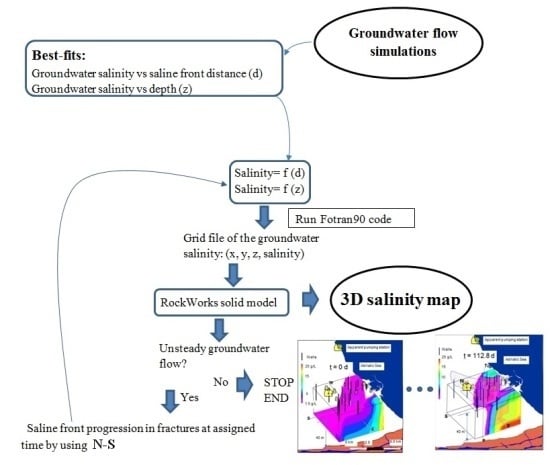
2. Methodology
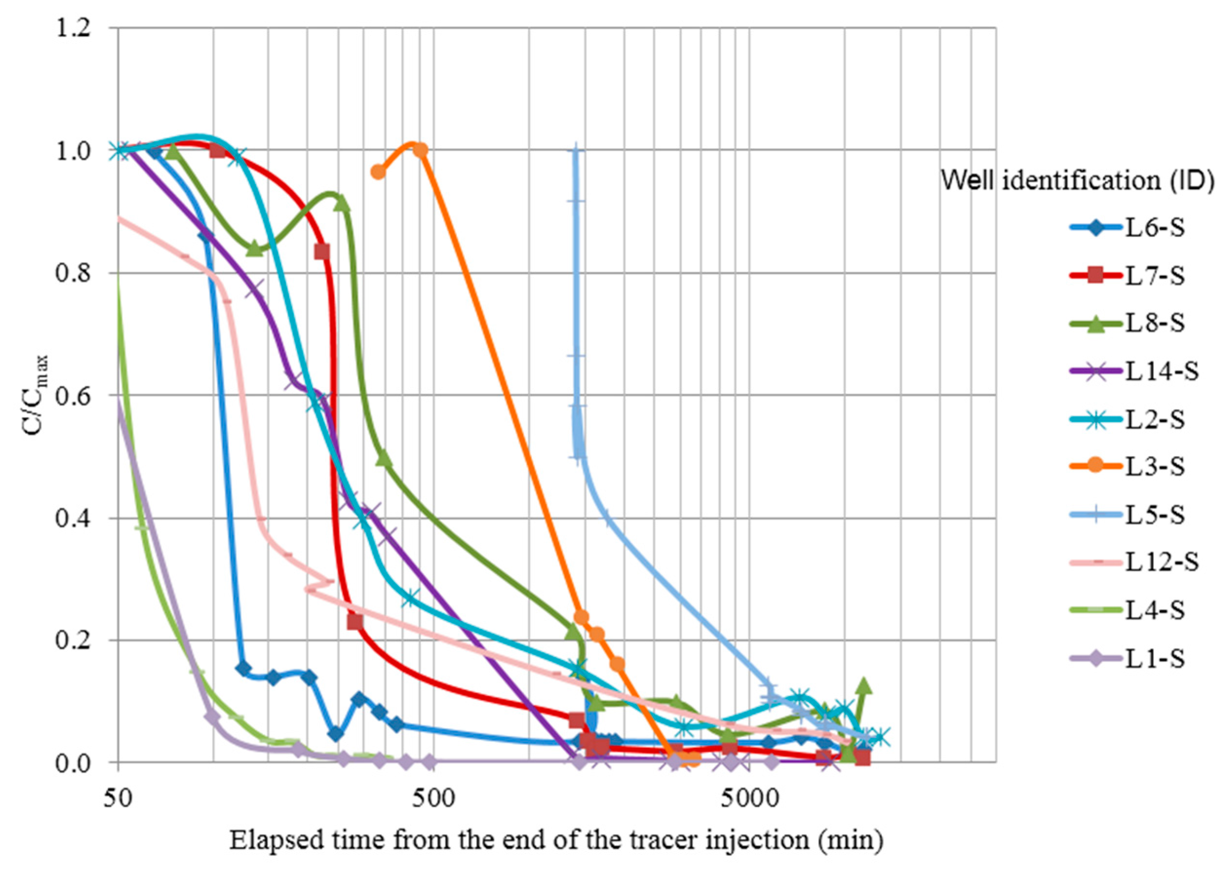
3. The Case Study and Field Tests
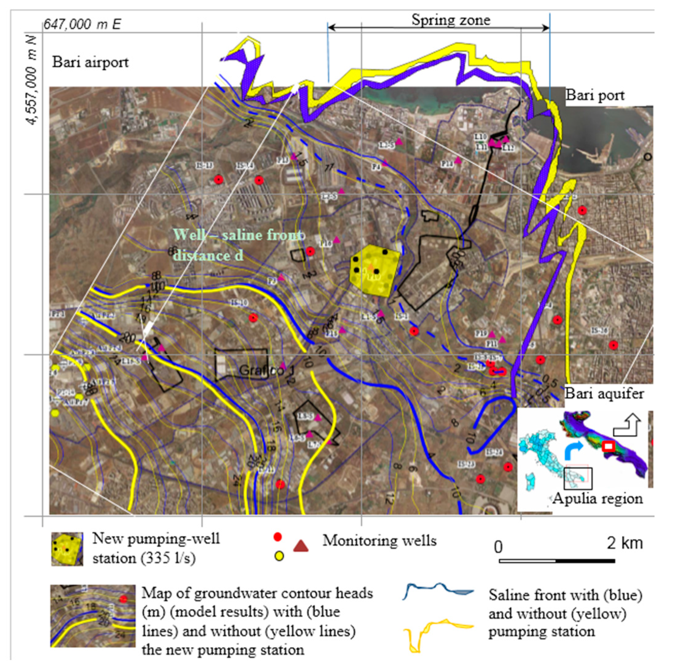
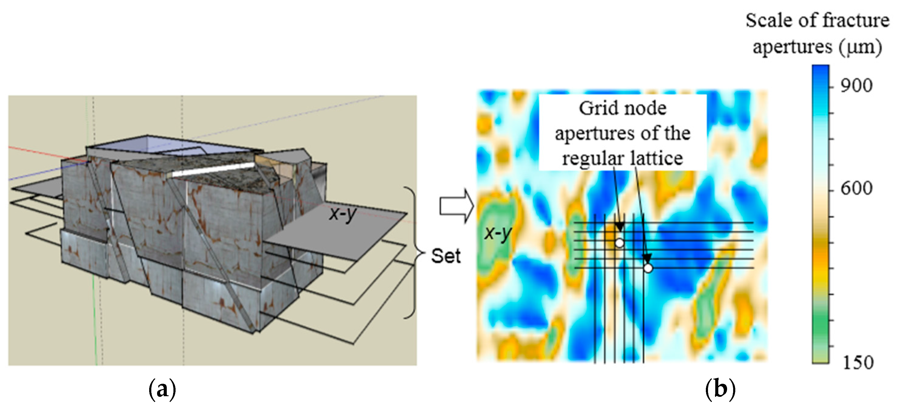
3.1. Field Set Up


| Well ID | Coordinates (UTM) | Tracer Test | Internal Diameter (m) | Piezometric Head (m above Sea Level) January–February 2012 | Aquifer Hydraulic Transmissivity (m2/s) | Ground Water Specific Discharge (m/day) | ||
|---|---|---|---|---|---|---|---|---|
| E | N | |||||||
| P10 | 652,892.8 | 4,553,271.3 | 0.300 | 4.480 | 0.09 | |||
| L1-S | 652,994.3 | 4,552,693.5 | X | 0.180 | 4.268 | 5.278 | 0.6 × 10⁻³ ± 1.8 × 10⁻⁴ | 1.3 |
| P11 | 654,726.9 | 4,552,308.3 | >1.0 | 1.251 | 1.611 | 0.02 | ||
| P19 | 654,580.1 | 4,552,382.9 | >1.0 | 0.77 | 1.110 | 0.02 | ||
| P14 | 654,093.3 | 4,554,883.8 | 0.012 | 0.311 | 0.321 | 0.045 | ||
| L2-S | 653,252.5 | 4,555,151.7 | X | >1.0 | 0.582 | 0.722 | 0.047 ± 0.01 | 0.5 |
| P4 | 653,053.8 | 4,554,841.5 | 0.012 | 0.266 | 0.386 | 0.06 | ||
| L3-S | 652,431.0 | 4,554,429.8 | X | >1.0 | 1.903 | 2.163 | 0.043 ± 0.02 | 2.6 |
| P3 | 651,569.2 | 4,553,208.7 | 0.300 | 4.321 | 5.441 | 0.07 | ||
| P16 | 652,360.0 | 4,553,741.7 | 0.014 | 2.658 | 3.538 | 0.09 | ||
| L4-S | 652,850.9 | 4,553,352.7 | X | 0.300 | 2.535 | 3.450 | 0.033 ± 0.03 | 2.2 |
| P18 | 652,442.4 | 4,552,454.1 | 0.200 | 6.926 | 0.07 | |||
| L5-S | 647,930.7 | 4,551,813.2 | X | 0.325 | 33.649 | 3.0 × 10⁻³ ± 1.8 × 10⁻³ | 0.2 | |
| L8-S | 652,094.5 | 4,551,194.2 | X | 0.080 | 8.532 | 0.02 ± 0.01 | 0.4 | |
| L7-S | 652,237.3 | 4,550,862.3 | X | 0.080 | 7.880 | 0.5 × 10⁻² ± 0.4 × 10⁻² | 0.6 | |
| L6-S | 651,974.4 | 4,550,961.1 | X | 0.080 | 8.892 | 0.11 ± 0.01 | 1.4 | |
| P13 | 651,750.4 | 4,554,936.6 | 0.300 | 0.807 | 0.02 | |||
| L9 | 654,682.2 | 4,555,123.7 | 0.100 | 0.705 | 0.1 | |||
| L10 | 654,572.7 | 4,555,144.1 | 0.100 | 0.167 | 0.01 | |||
| L11 | 654,588.5 | 4,555,126.1 | 0.100 | 0.317 | 0.01 | |||
| L12-S | 654,679.5 | 4,555,109.1 | X | 0.300 | 0.360 | 0.01 ± 0.7 × 10⁻³ | 0.3 | |
| L13 | 654,777.0 | 4,555,188.8 | 0.100 | 0.418 | 1.2 × 10⁻⁵ | |||
| L14-S | 649,860.6 | 4,552,197.6 | X | 0.080 | 34.370 | 1.1 × 10⁻⁴ ± 5.3 × 10⁻⁵ | 0.6 | |
| L15 | 649,623.8 | 4,552,059.7 | 0.080 | 35.260 | 1.2 × 10⁻⁵ | |||
| P2 | 651,595.4 | 4,551,934.3 | 0.300 | 6.760 | 0.025 | |||
3.2. Experiment Methodology
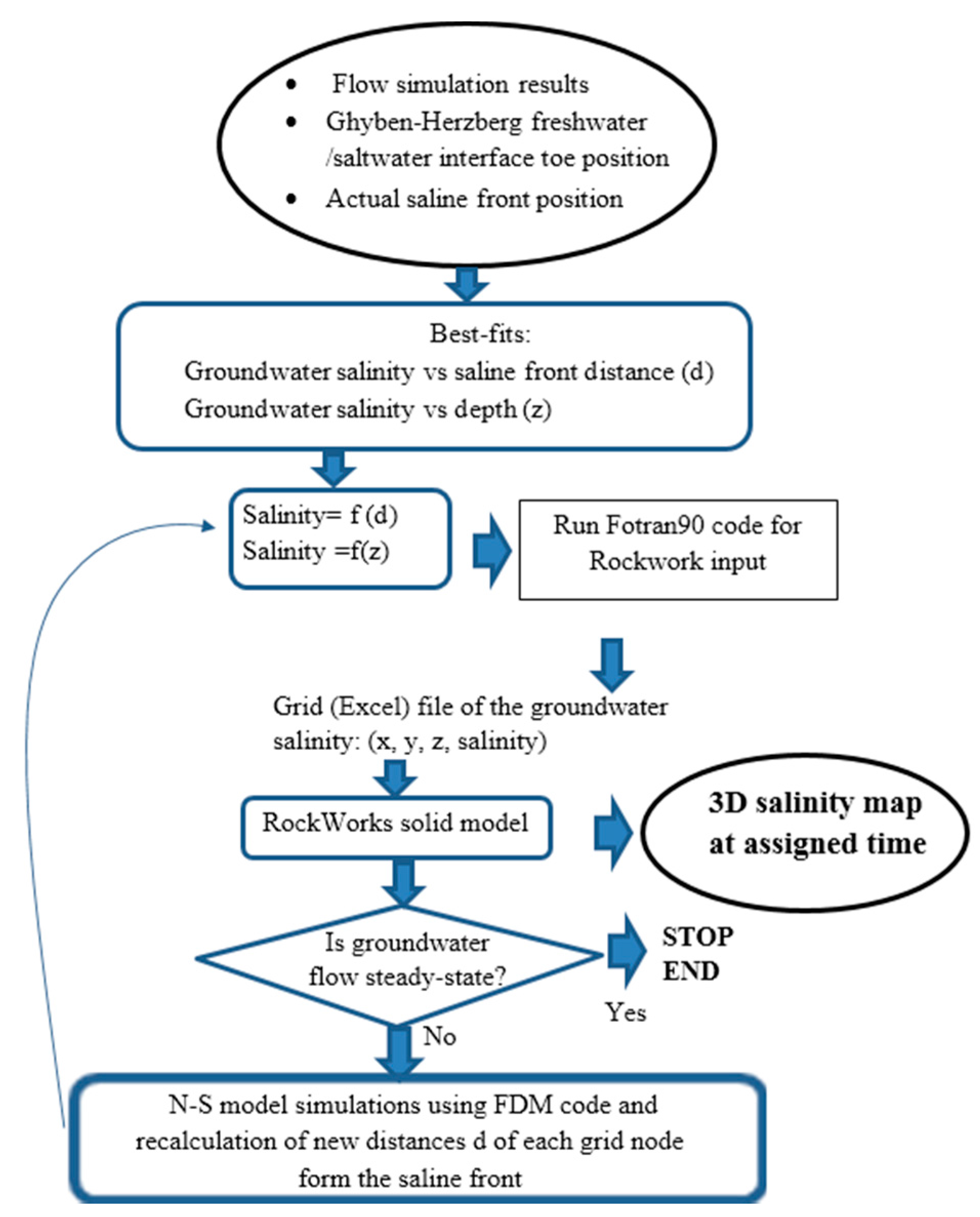
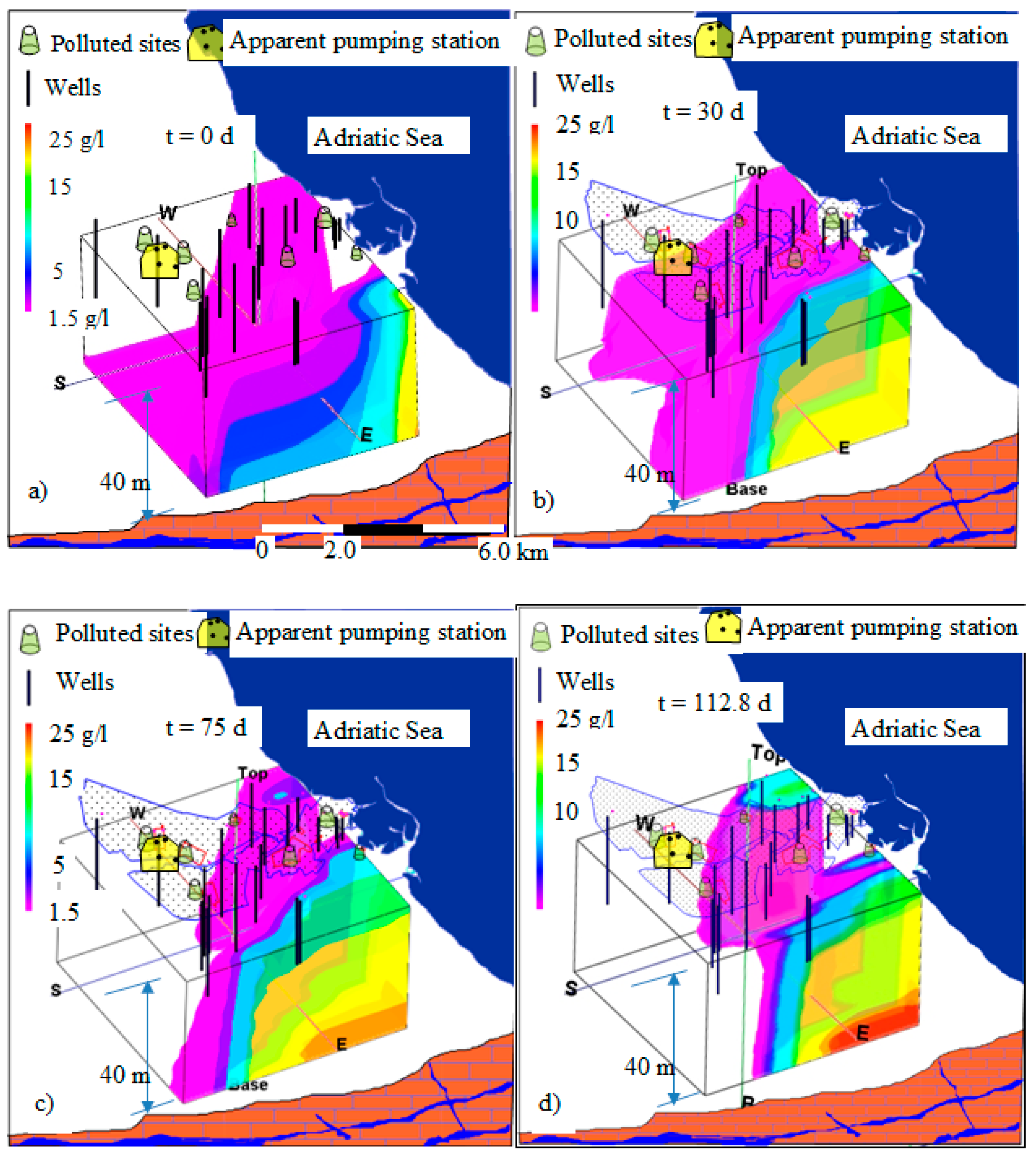
4. Groundwater Flow Simulation and Ghyben-Herzberg Interface Toe Position
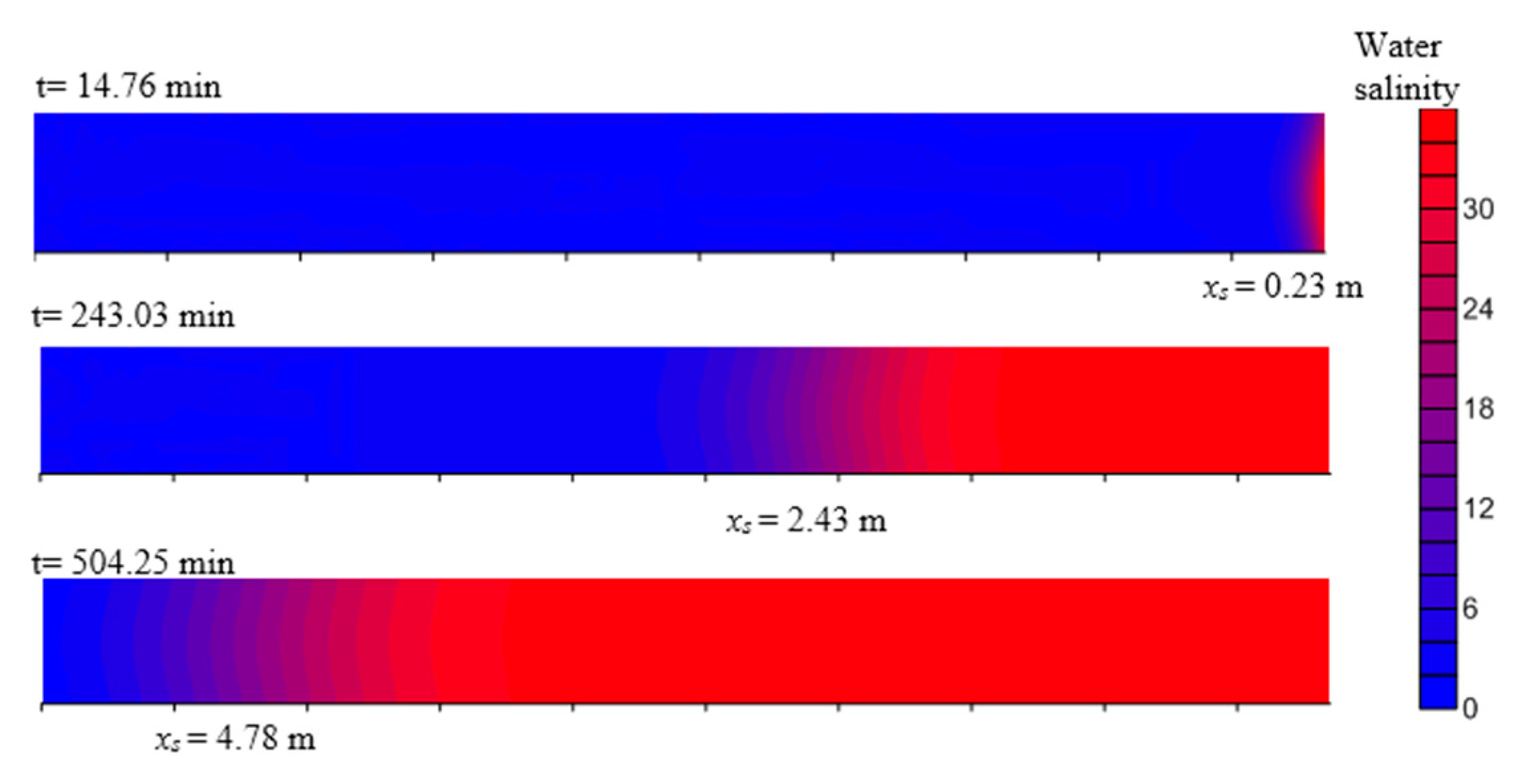
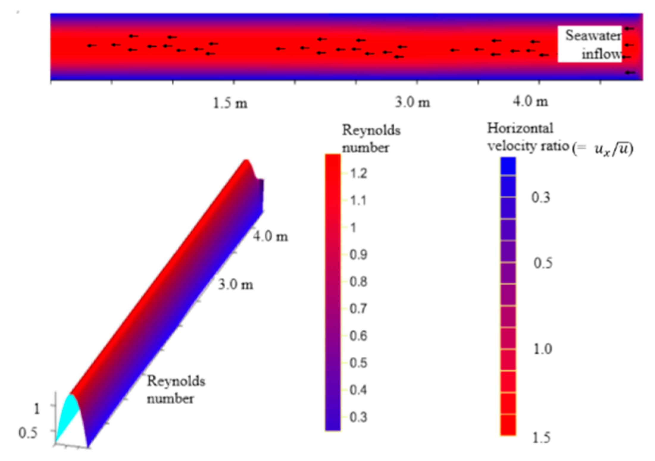
Advancement of Saline Front in a Fracture Using N-S
5. Conversion of Distances from Interface into Groundwater Salinity Data
5.1. Field Monitored Data
5.2. Ghyben-Herzberg Data
| ID Borehole | Actual (Winter 2012) Groundwater Salinity (g·L−1) at Different Water Depths | ||||||||
|---|---|---|---|---|---|---|---|---|---|
| 1 m | 11 m | 31 m | |||||||
| Mod | Mea | ±SD | Mod | Mea | ±SD | Mod | Mea | ±SD | |
| L1-S | 0.9 | 1.54 | 0.46 | 1.06 | 1.65 | 0.41 | 1.31 | ||
| P11 | 2.76 | 2.99 | 0.16 | 3.14 | 3.9 | ||||
| P19 | 3.75 | 3.71 | 0.03 | 4.27 | 5.29 | ||||
| L2-S | 3.12 | 2.63 | 0.34 | 3.55 | 4.39 | ||||
| L3-S | 2.11 | 3.40 | 0.91 | 2.4 | 2.97 | ||||
| L4 | 0.98 | 1.05 | 0.05 | 1.1 | 1.72 | 0.44 | 1.38 | 2.77 | 0.98 |
| L8-S | 0.5 | 0.71 | 0.15 | 0.52 | 0.65 | ||||
| L7-S | 0.5 | 0.58 | 0.06 | 0.6 | 0.74 | ||||
| L6-S | 0.5 | 0.67 | 0.12 | 0.52 | 0.78 | 0.19 | 0.65 | ||
| L9 | 2.02 | 1.54 | 0.34 | 2.3 | 2.85 | ||||
| L14-S | 0.93 | 0.59 | 0.24 | 1.06 | 0.56 | 0.35 | 1.31 | 1.03 | 0.20 |
| L15-S | 0.93 | 0.86 | 0.05 | 1.06 | 0.95 | 0.08 | 1.31 | 1.75 | 0.31 |
| L5-S | 0.5 | 0.63 | 0.09 | 0.52 | 0.68 | 0.12 | 0.65 | 1.50 | 0.60 |
| L12 | 2.02 | 0.56 | 1.03 | 2.3 | 2.26 | 0.03 | 2.85 | ||
| Mean | 1.53 | ±0.32 | 1.23 | ±0.23 | 1.76 | ±0.52 | |||
5.3. Data from Solutions of N-S Equations

6. Discussion and Conclusions
Acknowledgments
Author Contributions
Conflicts of Interest
References
- Barlow, P.M.; Reichard, E.G. Saltwater intrusion in coastal regions of North America. Hydrogeol. J. 2010, 18, 247–260. [Google Scholar] [CrossRef]
- Goswami, R.R.; Clement, T.P. Laboratory-scale investigation of saltwater intrusion dynamics. Water Resour. Res. 2007. [Google Scholar] [CrossRef]
- Essink, G.H.P.O. Salt water intrusion in a three-dimensional groundwater system in The Netherlands: A Numerical Study. Transp. Porous Media 2001, 43, 137–158. [Google Scholar] [CrossRef]
- Panyor, L. Renewable energy from dilution of salt water with fresh water: Pressure Retarded Osmosis. Desalination 2006, 199, 408–410. [Google Scholar] [CrossRef]
- Buonasorte, G. Development of geothermal energy in Italy until 2008 and short-term prospects, Ferrara (I). In Proceedings of the Congresso Internazionale: La Geotermia in Italia e in Europa. Quale futuro?—GEO THERM EXPO2009, Ferrara, Italy, 23 September 2009.
- Chongo, M.; Wibroe, J.; Staal-Thomsen, K.; Moses, M.; Nyambe, I.A.; Larsen, F.; Bauer-Gottwein, P. The use of Time Domain Electromagnetic method and Continuous Vertical Electrical Sounding to map groundwater salinity in the Barotse sub-basin, Zambia. Phys. Chem. Earth 2011, 36, 798–805. [Google Scholar] [CrossRef]
- I-GIS. GeoScene3D—Modelling and Visualization of Geological Data, Risskov, Denmark (DK). Available online: http://www.i-gis.dk/GeoScene3D (accessed on 3 February 2016).
- Hydrogeophysics-Group-1. Getting Started with SiTEM and SEMDI; Denmark University of Aarhus: Aarhus, Denmark, 2001. [Google Scholar]
- Geomoto Software. Res2Dinv v. 3.54 for Windows 98/Me/2000/NT/XP, Gelugor, Penang, Malaysia. Available online: http://www.geoelectrical.com (accessed on 3 February 2016).
- Mullen, I.; Kellet, J. Groundwater salinity mapping using airborne electromagnetics and borehole data within the lower Balonne catchment, Queensland, Australia. Int. J. Appl. Earth Obs. Geoinform. 2007, 9, 116–123. [Google Scholar] [CrossRef]
- Archie, G.E. The electrical resistivity log as an aid in determining some reservoir characteristics. Trans. Am. Inst. Mech. Eng. 1942, 146, 54–67. [Google Scholar] [CrossRef]
- Lesch, S.M.; Strauss, D.J.; Rhoades, J.D. Spatial prediction of soil salinity using electromagnetic induction techniques 1. Statistical prediction models: A comparison of multiple linear regression and cokriging. Water Resour. Res. 1995, 2, 373–386. [Google Scholar] [CrossRef]
- Masciopinto, C.; la Mantia, R.; Chrysikopoulos, C.V. Fate and transport of pathogens in a fractured aquifer in the Salento area, Italy. Water Resour. Res. 2008. [Google Scholar] [CrossRef]
- Masciopinto, C. Simulation of coastal groundwater remediation: The Case of Nardò Fractured Aquifer in Southern Italy. Environ. Model. Softw. 2006, 21, 85–97. [Google Scholar] [CrossRef]
- Masciopinto, C.; Volpe, A.; Palmiotta, D.; Cherubini, C. A combined PHREEQC-2/parallel fracture model for the simulation of laminar/non-laminar flow and contaminant transport with reactions. J. Contam. Hydrol. 2010, 117, 94–108. [Google Scholar] [CrossRef]
- Masciopinto, C.; Palmiotta, D. Relevance of solutions to the Navier-Stokes equations for explaining groundwater flow in fractured karst aquifers. Water Resour. Res. 2013. [Google Scholar] [CrossRef]
- Walther, M.; Delfs, J.O.; Grundmann, J.; Kolditz, O.; Lied, R. Saltwater intrusion modeling: Verification and Application to an Agricultural Coastal Arid Region in Oman. J. Comput. Appl. Math. 2012, 236, 4798–4809. [Google Scholar] [CrossRef]
- Werner, A.D.; Bakker, M.; Post, V.E.A.; Vandenbohede, A.; Lu, C.; Ataie-Ashtiani, B.; Simmons, C.; Barry, D.A. Seawater intrusion processes, investigation and management: Recent Advances and Future Challenges. Adv. Water Resour. 2013, 51, 3–26. [Google Scholar] [CrossRef]
- Masciopinto, C.; Palmiotta, D. Flow and Transport in Fractured Aquifers: New Conceptual Models Based on Field Measurements. Transp. Porous Media 2012. [Google Scholar] [CrossRef]
- Mehta, A. Ultraviolet-Visible (UV-Vis) Spectroscopy—Derivation of Beer-Lambert Law. Available online: http://pharmaxchange.info/press/2012/04/ultraviolet-visible-uv-vis-spectroscopy-%E2%80%93-derivation-of-beer-lambert-law/ (accessed on 3 February 2016).
- Chaniotis, A.K.; Frouzakis, C.E.; Lee, J.C.; Tomboulides, A.G.; Poulikakos, D.; Boulouchos, K. Remeshed smoothed particle hydrodynamics for the simulation of laminar chemically reactive flows. J. Comput. Phys. 2003, 191, 1–17. [Google Scholar] [CrossRef]
- Gesteira, M.G.; Rogers, B.D.; Dalrymple, R.A.; Crespo, A.J.C.; Narayanaswamy, M. SPHysics v2.0, January 2010: Open-Source Smoothed Particle Hydrodynamics Code. Available online: http://wiki.manchester.ac.uk/sphysics/index.php (accessed on 3 February 2016).
- Meyers, J.; Geurts, B.J.; Baelmans, M. Optimality of the dynamic procedure for large-eddy simulations, American Institute of Physics. Phys. Fluids 2005. [Google Scholar] [CrossRef]
- Becker, M.; Teschner, M. Weakly Compressible SPH for Free Surface Flows. In Proceedings of the Euro graphics/ACM SIGGRAPH Symposium on Computer Animation, Aire-la-Ville, Switzerland, 3–4 August 2007.
- Boersma, B.J. A 6th order staggered compact finite difference method for the incompressible Navier-Stokes and scalar transport equations. J. Comput. Phys. 2011. [Google Scholar] [CrossRef]
- Watson, T.A.; Werner, A.D.; Simmons, C.T. Transience of sea water intrusion in response to sea level rise. Water Resour. Res. 2010. [Google Scholar] [CrossRef]
- Yechieli, Y.; Shalev, E.; Wollman, S.; Kiro, Y.; Kafri, U. Response of the Mediterranean and Dead Sea coastal aquifers to sea level variations. Water Resour. Res. 2010. [Google Scholar] [CrossRef]
- Zlotnik, V.A.; Robinson, N.I.; Simmons, C.T. Salinity dynamics of discharge lakes in dune environments: Conceptual Model. Water Resour. Res. 2010. [Google Scholar] [CrossRef]
© 2016 by the authors; licensee MDPI, Basel, Switzerland. This article is an open access article distributed under the terms and conditions of the Creative Commons by Attribution (CC-BY) license (http://creativecommons.org/licenses/by/4.0/).
Share and Cite
Masciopinto, C.; Palmiotta, D. A New Method to Infer Advancement of Saline Front in Coastal Groundwater Systems by 3D: The Case of Bari (Southern Italy) Fractured Aquifer. Computation 2016, 4, 9. https://doi.org/10.3390/computation4010009
Masciopinto C, Palmiotta D. A New Method to Infer Advancement of Saline Front in Coastal Groundwater Systems by 3D: The Case of Bari (Southern Italy) Fractured Aquifer. Computation. 2016; 4(1):9. https://doi.org/10.3390/computation4010009
Chicago/Turabian StyleMasciopinto, Costantino, and Domenico Palmiotta. 2016. "A New Method to Infer Advancement of Saline Front in Coastal Groundwater Systems by 3D: The Case of Bari (Southern Italy) Fractured Aquifer" Computation 4, no. 1: 9. https://doi.org/10.3390/computation4010009
APA StyleMasciopinto, C., & Palmiotta, D. (2016). A New Method to Infer Advancement of Saline Front in Coastal Groundwater Systems by 3D: The Case of Bari (Southern Italy) Fractured Aquifer. Computation, 4(1), 9. https://doi.org/10.3390/computation4010009