CFD Simulation and Experimental Analyses of a Copper Wire Woven Heat Exchanger Design to Improve Heat Transfer and Reduce the Size of Adsorption Beds

Abstract

The chief objective of this study is the proposal design and CFD simulation of a new compacted copper wire woven fin heat exchanger and silica gel adsorbent bed used as part of an adsorption refrigeration system. This type of heat exchanger design has a large surface area because of the wire woven fin design. It is estimated that this will help improve the coefficient of performance (COP) of the adsorption phase and increase the heat transfer in this system arrangement. To study the heat transfer between the fins and porous adsorbent reactor bed, two experiments were carried out and matched to computational fluid dynamics (CFD) results.

1. Introduction

This article attempts to provide insight into the working principles of a wire woven heat exchanger used in an adsorption cooling system. The installation procedure for a test rig equipped with a data logging system has been specified along with the calibration of sensors. Subsequently, the method followed in conducting tests on a new configuration of adsorption cooling system is described. The purpose of testing the system is to ascertain systems viability and interaction of individual components. The tests also were carried out to determine the test rig parameter for use in a CFD simulation. Several routine curves were generated for system components such as the adsorbent bed evaporator and condenser.

In recent years, many researchers have investigated the enhancement of the thermal conductivity of porous adsorbent beds in the hope of improving the thermal performance of such systems [1]. Mass transfer restrictions are also significant in manipulating the performance of this cooling technology [2,3,4,5,6]. It is of late that computational fluid dynamics (CFD) research has been presented [7,8,9]. In these studies, Darcy’s law [7,8] and the extended Darcy-Ergun equation [10] were adopted as the momentum equation for water vapour flow in the porous adsorbent. However, Darcy’s law is appropriate only for incompressible fluids. Past research studies have not clearly investigated the thermal heat transfer of porous adsorbent bed in relation to the effect of the adsorbed presence of the water vapour within the adsorbent.

Since the heat and mass transfer properties are greatly affected by the construction of the adsorbent bed heat exchanger, the equivalent thermal conductivity should be defined as a function of the configuration parameters. In this research study, an experimental test rig and a 3D model were used to describe the heat transfer in an adsorbent bed. The solution from the experimental test rig and the CFD model will be used to optimize the configuration of the adsorbent bed and the operating conditions [10].

2. Experimental Setup

The adsorption test rig consists of a condenser, evaporator and adsorbent bed. The adsorbent bed contains a heat exchanger consisting of one silica gel filled copper wire woven finned heat exchanger. The wire-finned heat exchanger contains 0.5 kg of silica gel in total. Heating and cooling water tanks are used to provide the adsorption bed, condenser and evaporator with water at the desired temperatures. During the desorption stage of the cycle, the adsorption bed is heated to the temperature (80 °C) while the condenser is kept at 25 °C [1,4,5,6,7,8,9,10,11,12,13,14,15,16,17]. During the adsorption stage of the cycle, the adsorption bed is cooled down to 25 °C and the evaporator to 15 °C [14,10]. Valves with a timer are used to control the heating and cooling water between the cycles of operation of the adsorbent bed, evaporator and condenser [10].

Components

The experimental test rig setup for adsorption cooling system measurements consisted of the following components [10]:

• One adsorbent bed;
• Evaporator;
• Condenser;
• Three water tanks one hot water tank, one cooling water tank and one chilled water tank;
• Vacuum pump;
• Manually switchable valves, solenoid valves and one diaphragm valve;
• Sensors: Flow meters, pressure transducer and type K thermocouple;
• Measuring: data logger (multiplexes with digital converter) transferring data to a personal computer.

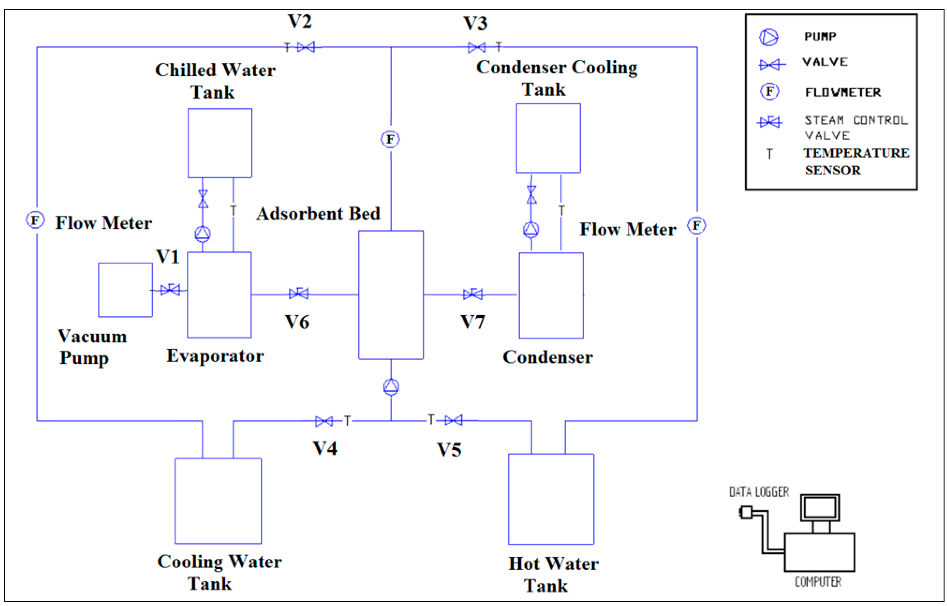
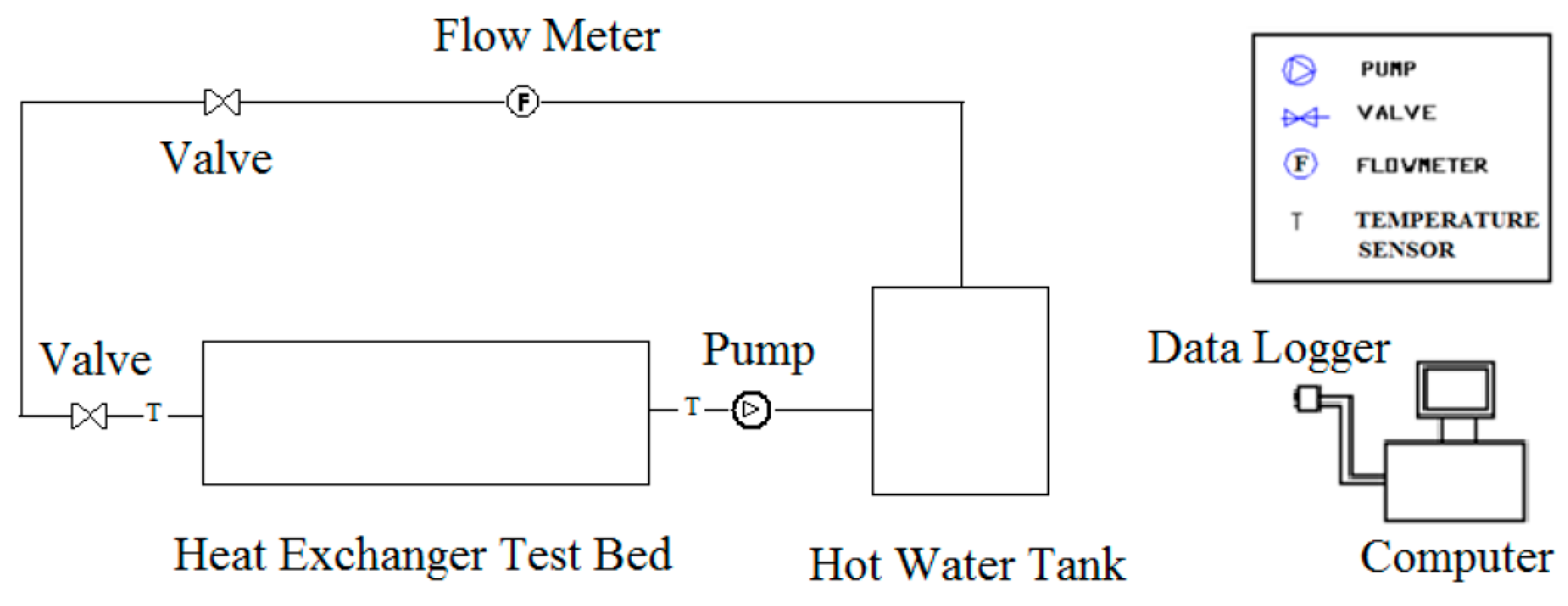
One flow meter is installed in each water system. Valves V2 and V3 act as the controllers for the flow rates. The heat source is provided by a wire wound tube heat exchanger that is heated by the heating coil. Hot water temperature is controlled by valve V5 [10].

Valve V1 controls the temperature of the chilled water. The controlled operation of the vacuum valves and the valves in heating and cooling water system are controlled by a Programme logic controller (PLC) system. Please see Figure 1 for Schematic view of the adsorption cooling test rig with the wire woven fins. The temperature of the cooling water is about 25 °C, and the hot water temperature is 80 °C.

Figure 1. Schematic view of the adsorption cooling test rig with the wire woven fins.

Figure 1. Schematic view of the adsorption cooling test rig with the wire woven fins.

3. Heat Transfer Coefficients and Performance Modelling

The heat transfer coefficients of the adsorption of water vapour and the desorption of water vapour are calculated from the experimentally measured temperatures of the porous adsorbent. The formula for the heat transfer coefficient using log mean temperature difference is given by [6,9,10,11,12,13,14,15,16,17].

$$U_{overall}=\frac{Q_{des/ads}}{A_{Bed}LMTD}$$

(1)

where U_overall is the overall heat transfer coefficient, Q_des/ads is the desorption or adsorption heat, A_Bed is the surface area and fin area of the porous adsorbent bed and LMTD is the log mean T temperature difference is as [10].

$$LMTD=\frac{\left(T_{hw/cw}-T_{des/ads}\right)-\left(T_{hw/cw,out}-T_{des/ads}\right)}{In\frac{\left(T_{hw/cw}-T_{des/ads}\right)}{\left(T_{hw/cw,out}-T_{des/ads}\right)}}$$

(2)

The adsorption and desorption heat of the system are estimated using the inlet and outlet temperatures of the adsorbent beds, and are given by

$$Q_{des/ads}={\mathsf{ṁ}}_{hw/cw}{C}_P\left(T_{des/ads}\right)\left(T_{hw/cw,in}-T_{hw/cw,out}\right)$$

(3)

Here ṁ_hw/cw is the flow of the hot water or cooling water flowing into the porous adsorbent bed and C_P(T_des/ads) is the heat of the water temperature passing through the porous adsorbent bed. The heat transfer for adsorption and desorption of water vapour processes are measured from the returning steady state temperatures of the AD cycle [9,10,11,12,13,14,15,16,17,18].

The performance of the adsorption cooling is obtained by using the key performance parameters, namely the (SCC) specific cooling capacity and the (COP) coefficient of performance that are given as follows,

$$SCC=\underset{0}{\overset{t_{cycle}}{{\displaystyle \int }}}\frac{Q_{eva{p}^{\tau }}}{M_{\text{sg}}}dt$$

(4)

$$Q_{evap}=\mathsf{ṁ}{}_{chilled}{C}_P\left(T_{evap}\right)\left(T_{chilled,in}-T_{chilled,out}\right)$$

(5)

$$COP=\underset{0}{\overset{t_{cycle}}{{\displaystyle \int }}}\frac{Q_{eva{p}^{\tau }}}{Q_{des}}dt$$

(6)

where ṁ_chilled is the chilled water flow rate and Q_evap is the heat of evaporation of the water in the evaporator chamber. The heat of condensation of the water is calculated using cooling water inlet and outlet temperatures and flow rate of the condenser chamber, and it is stated as the following.

$${\mathrm{Q}}_{\text{evap}}={\mathsf{ṁ}}_{cond}{C}_P\left(T_{cond}\right)\left(T_{Cond,in}-T_{cond,out}\right)$$

(7)

4. Wire Wound Finned Tubes

A wire woven heat exchanger construction adopted for the adsorbent bed used as part of an adsorption cooling system makes use of a surface in the form of wire helically wound fins. Copper wire is used to give high conductivity and thus make the most of the efficiency of this form of extended surface.

For the purpose of this experiment a copper wire woven fin heat exchanger was manufactured from drawings to the specifications shown in Table 1, provided to P. A. K Engineering Limited (Staffordshire, UK), who donated it for the purpose of this study.

Table 1. Specification for the copper wire woven fins.

Tube Diameter	15 mm
Tube Material	Copper
Wire Material	Copper wire
Copper Thickness	0.7 mm
Loops per Turn	70 turns per fin pitch
Length of coPper Wire	1400 mm per fin pitch
Maximum Operation Temperature	120 °C

Table 1. Specification for the copper wire woven fins.

Tube Diameter	15 mm
Tube Material	Copper
Wire Material	Copper wire
Copper Thickness	0.7 mm
Loops per Turn	70 turns per fin pitch
Length of coPper Wire	1400 mm per fin pitch
Maximum Operation Temperature	120 °C

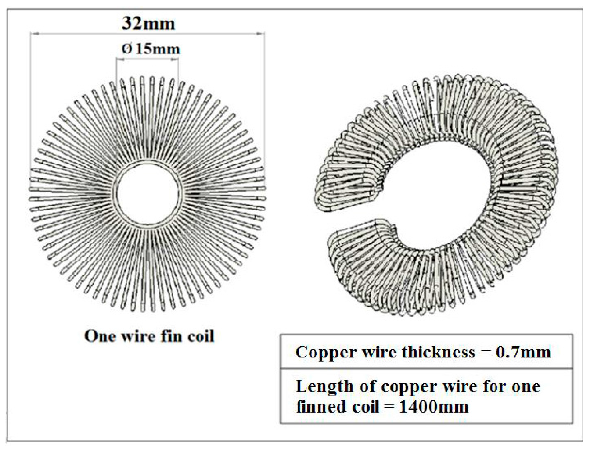
Table 1 shows the specification of the copper wire woven finned heat exchanger the copper tube diameter is 15 mm, and the thickness of the wire fin is 0.7 mm. The wire is made up of 70 loops per turn, 360 degrees; the length of the wire per 360 turns is 1400 mm, and one turn is the equivalent to one flat fin, so two turns of wire fins are one pitch. Figure 2 and Figure 3 show the stages of preparing the copper wire woven fin heat exchangers covered with silica gel for the experiment.

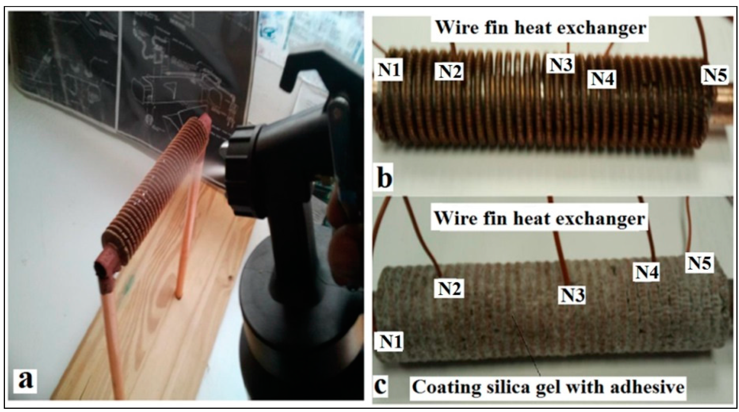
Figure 2. Wire wound heat exchanger being prepared for heat transfer testing. (a–c) Epoxy was used to attach silica gel to wire fin; this is a similar method to that used by (Source SorTech) [10].

Figure 2. Wire wound heat exchanger being prepared for heat transfer testing. (a–c) Epoxy was used to attach silica gel to wire fin; this is a similar method to that used by (Source SorTech) [10].

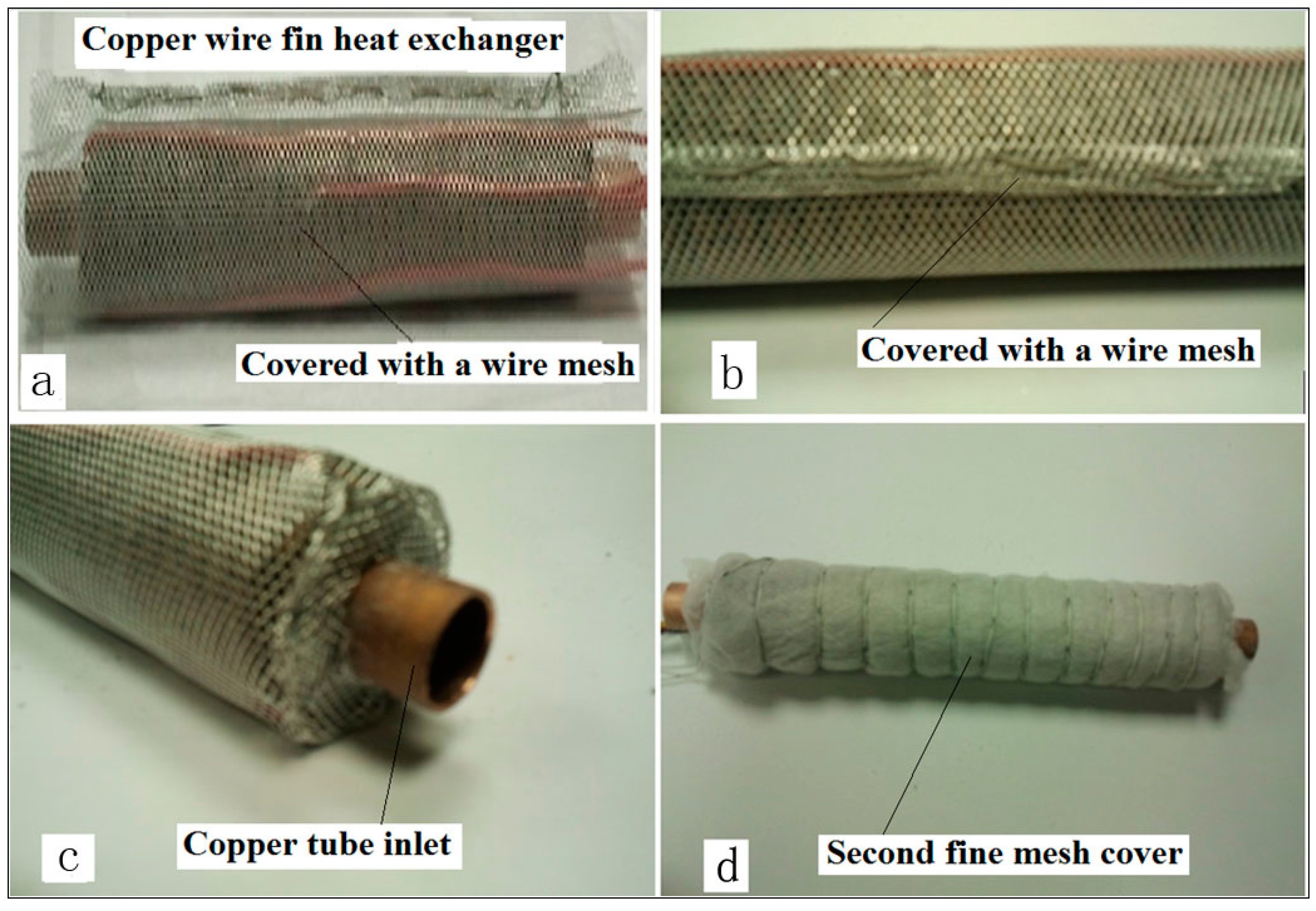
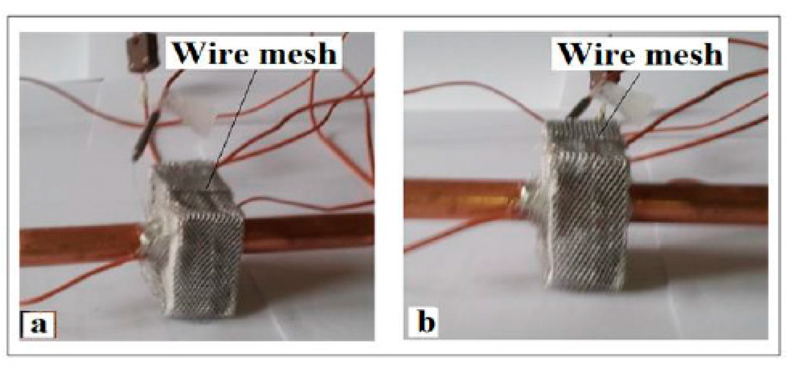
Figure 3. (a,b) Wire Aluminum mesh was used to cover the epoxy attach silica gel; (c,d) second covering of fine mesh.

Figure 3. (a,b) Wire Aluminum mesh was used to cover the epoxy attach silica gel; (c,d) second covering of fine mesh.

The advantages of using the epoxy resin to attach the silica gel granule to the wire fin heat exchanger are: (1) improved speed of heat transfer; (2) less volume and weight of silica gel; (3) improved vapour transport.

5. Systems Measuring Instruments and Measuring Points

The test rig incorporated several measuring instruments to produce a range of parameter boundary conditions for the CFD simulation. These are described further on in this section, where the various measuring points in the experiment are discussed [10].

5.1. Wire Fin and Thermocouple Positions

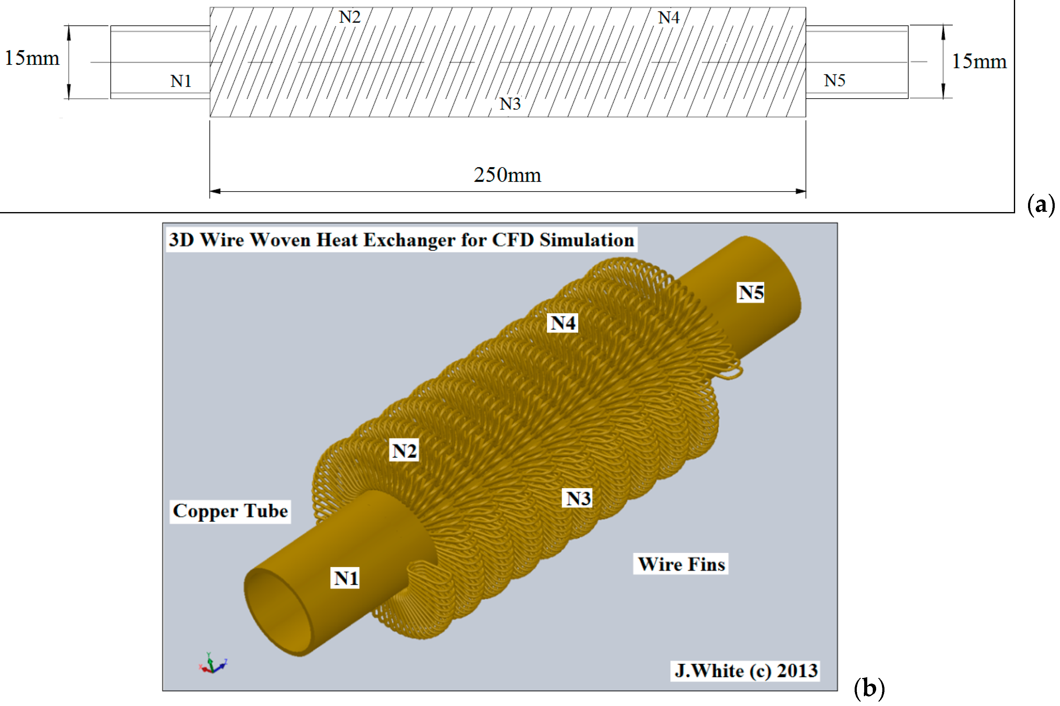
The data collected for the heat transfer performance evaluation of the wire woven fins heat exchanger was measured by attaching five K-type thermocouples at various points on the wire woven fins as shown in Figure 4 [9,10].

Figure 4. (a) A 2D representation of the location of the K-type thermocouples indicated with (N1, N2, N3, N4 and N5); (b) A 3D representation of the location of the K-type thermocouples indicated with (N1, N2, N3, N4 and N5).

Figure 4. (a) A 2D representation of the location of the K-type thermocouples indicated with (N1, N2, N3, N4 and N5); (b) A 3D representation of the location of the K-type thermocouples indicated with (N1, N2, N3, N4 and N5).

5.2. Temperatures

Listed here are the measuring point positioning in the experimental test rig:

• Five measuring points on the wire wound tubes heat exchanger;
• Two measuring points at opposite outside surfaces of the adsorbent;
• One measuring point at the flange fitting of the adsorbent bed;
• Ambient temperature;
• Inlet and outlet temperatures of the three coolants;
• Temperature of the liquid in the evaporator.

5.3. Temperature Sensors

All five temperature sensors were thermocouple type K. The sensors used in this system are embedded in the wire wound tube heat exchanger. The temperature range was from 25 °C up to 80 °C. The sensors provided the current of 1 mA (also measured by the data logger through a high precision resistance) through a constant current supply [3,10].

5.4. Vacuum Pressure Gauge and Solenoid Valves

With vacuum pressure gauges, the pressures in the evaporator, in the adsorbent bed and the condenser are recorded one after another. For this system, the sensor had four outlets connected with solenoid valves to the components. The data transducer controls the solenoid valves; this also has the control sequences from a PLC connected to a computer programme [10].

5.5. Flow Meters

In the coolant and heating circuits of the test rig, flow meters are installed: one turbine velocity flow meter and two acrylic water velocity flow meters [10].

5.6. The Data Logger

The measuring signals of all built-in sensors are scanned through multiple data acquisition system channels by a data logger and then transmitted to a computer [1,2,3,4,5,6,7,8,9,10,11,12,13,14,15,16,17,18].

5.7. Vacuum Pumps

For low-temperature evaporation of the working fluid, a vacuum pump was necessary. The vacuum pump is connected to the evaporator and adsorbent bed. A vacuum pump was used to reduce the pressure below the vapour pressure of the water at ambient temperature [10].

6. Wire Woven Fin Heat Exchanger Test Rig

An adsorption test rig is designed with an evaporator and condenser of identical construction. The reasons for designing this adsorption test rig is to compare the heat transfer performance of silica gel adsorbent and water pairs on wire wound tubes and then to use data for CFD simulation [10].

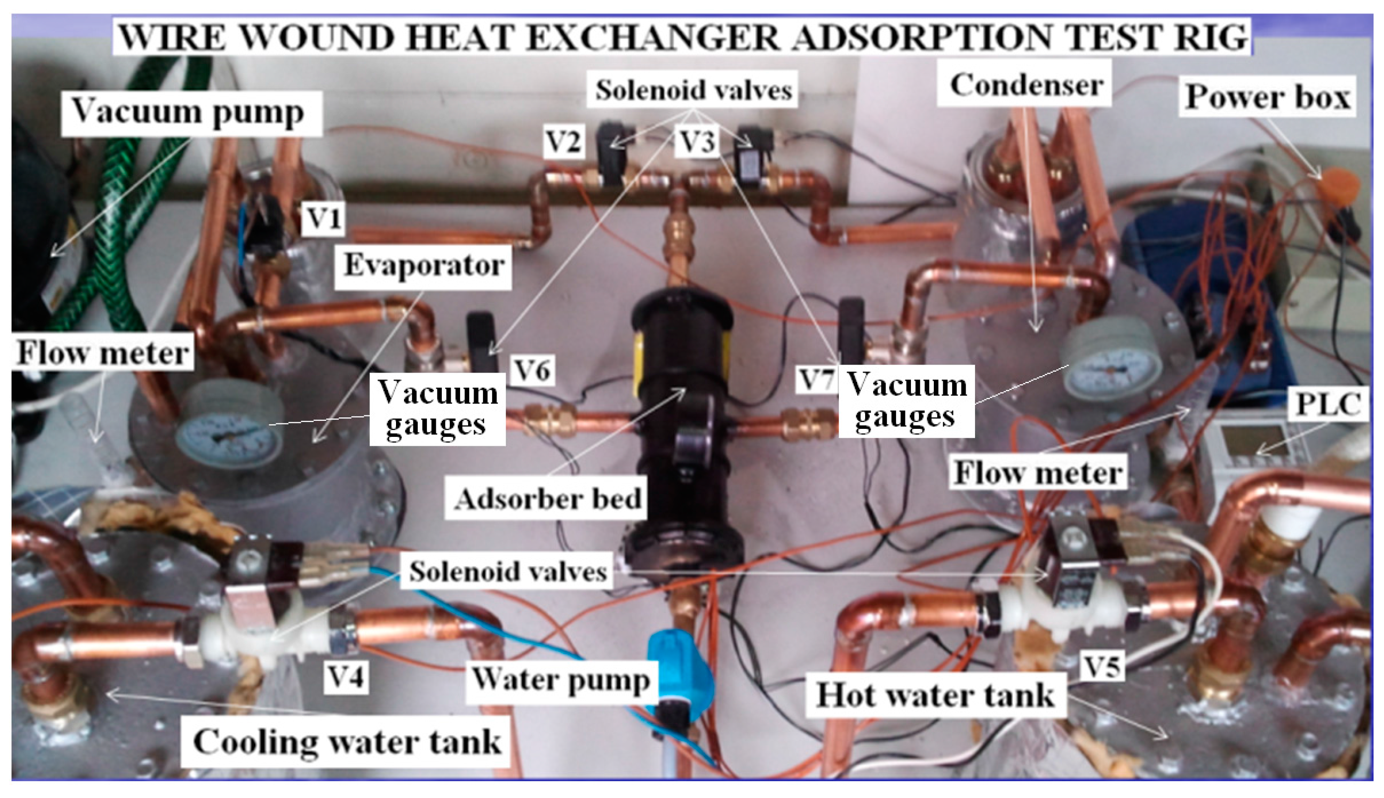
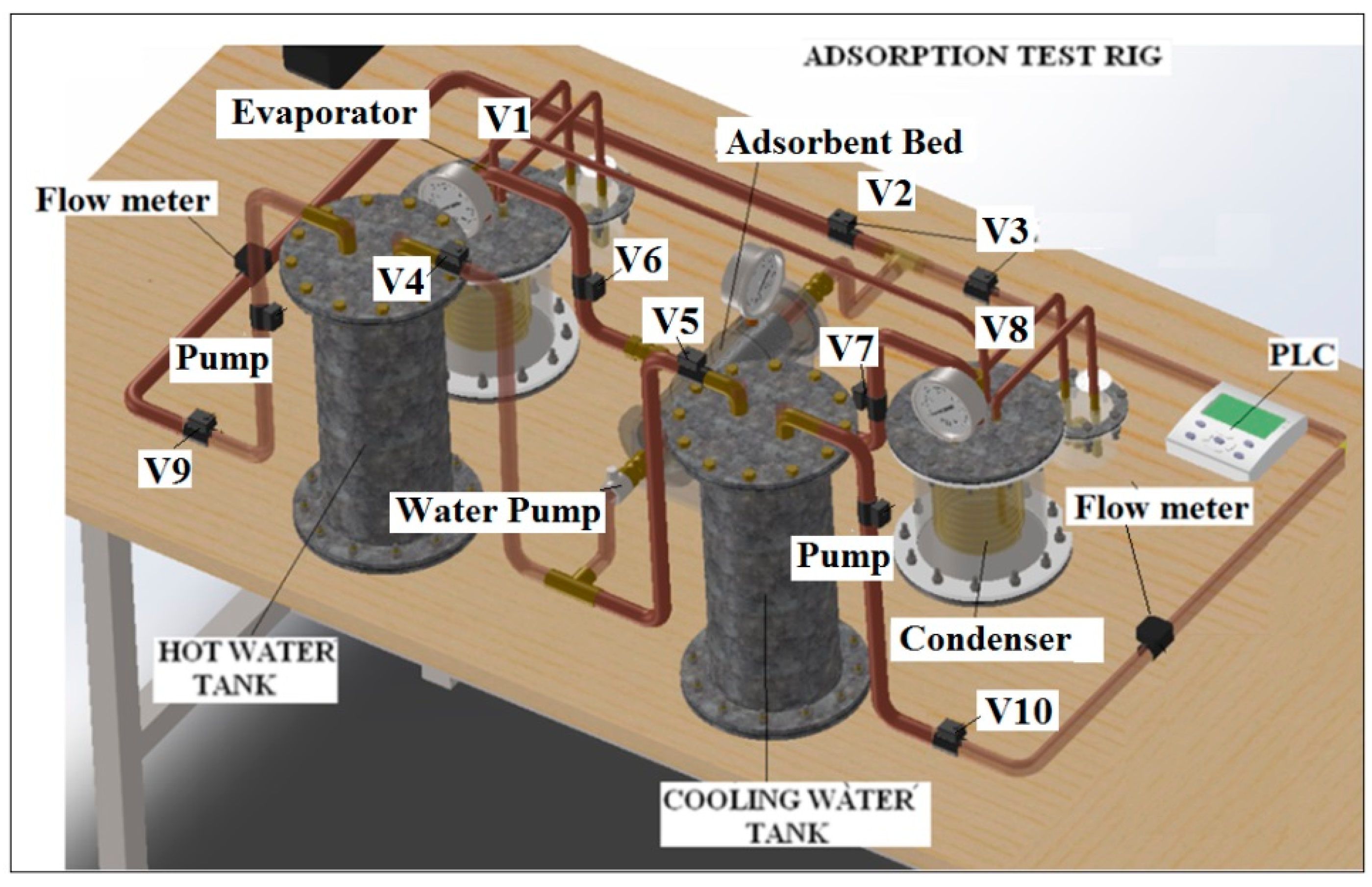
Figure 5 shows a labelled photograph of the adsorption test rig layout, the adsorbent bed and 3D CAD design are shown in Figure 6 and Figure 7, respectively. During the construction of the test rig, there was difficulty in obtaining a full vacuum in the evaporator because of leakage in the gaskets. The experiments were almost abandoned due to this problem; however, this problem was resolved by using epoxy resin pasted onto the gasket and permanently sealing the gaskets, allowing tests to be carried out. The drawback of this solution was that the evaporator is permanently locked. This is not a problem in this study because the test rig is a temporary prototype to generate data for the purpose of the CFD Simulation [10].

Figure 5. The adsorption bed test rig.

Figure 5. The adsorption bed test rig.

Figure 6. Helix copper coil heat exchanger (designed by J. White ©2012 [10]).

Figure 6. Helix copper coil heat exchanger (designed by J. White ©2012 [10]).

Figure 7. 3D Model of test rig design by John White ©2012 [10].

Figure 7. 3D Model of test rig design by John White ©2012 [10].

All the switch solenoid valves and vacuum pumps used in this adsorption cooling test equipment are controlled by a PLC programmer system connected to a computer. It is an automatically running prototype [10].

6.1. Testing Procedure

Before the experiment, the test equipment (evaporator, condenser, the adsorbent bed and piping systems) is first vacuumed by a vacuum pump for approximately one hour. For the duration of the evacuation, hot water at 85 °C is supplied to the porous adsorbent bed to heat-up the porous silica gel to remove moisture trapped in the adsorbent bed. When all moisture is completely removed, the test equipment was then ready for the experiment [10].

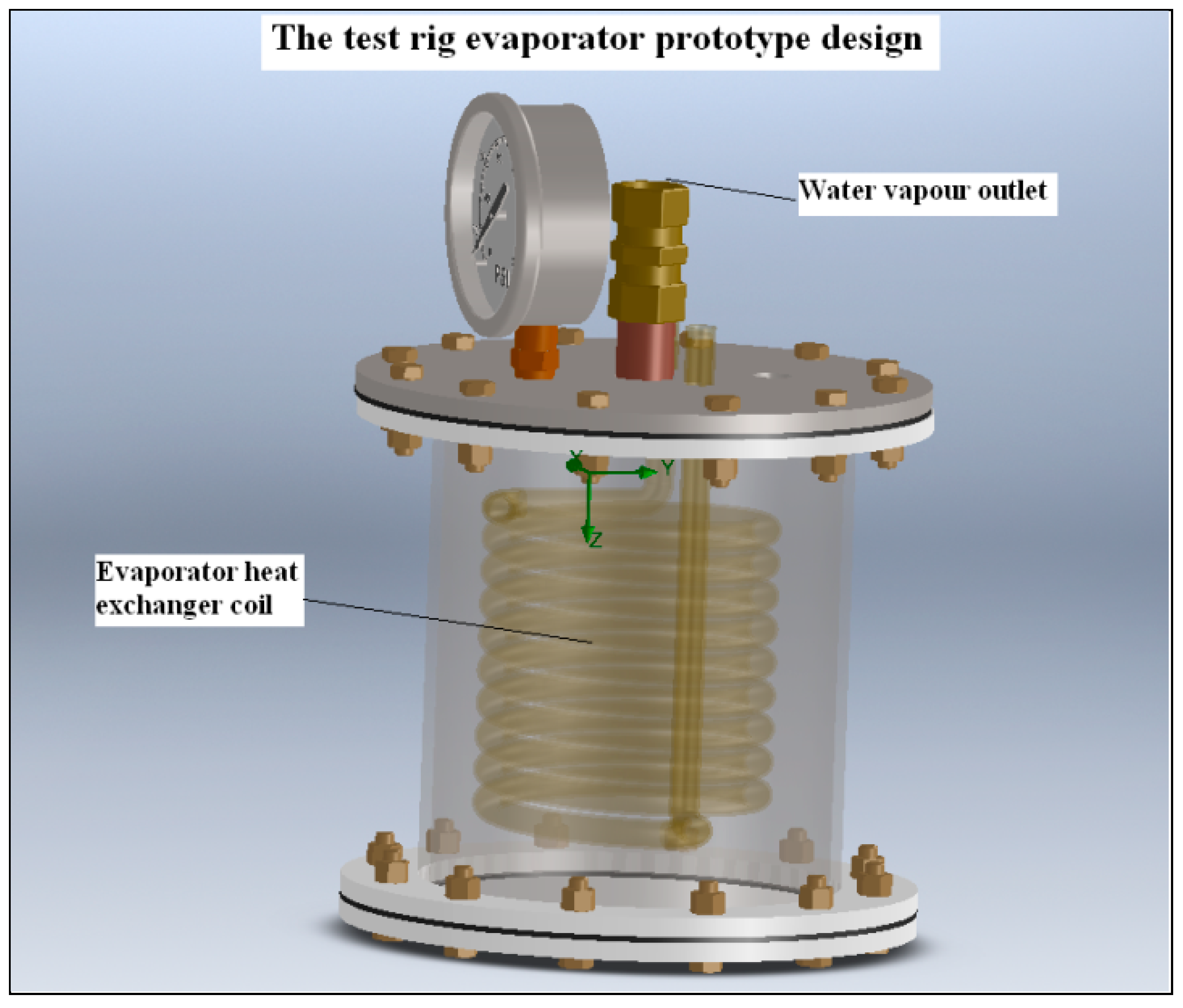
The adsorption cooling test rig was built with only one adsorbent bed; a copper wire woven finned heat exchanger is used for this adsorbent bed. The adsorbent material (silica gel) are filled in the spaces between the wire fins. The connection to the evaporator, adsorbent bed and condenser is by valves 6 and 7. The evaporator is a cylindrical vacuum chamber [10].

At the bottom of the vacuum chamber, a helix copper coil heats the exchanger as shown in Figure 6, this helix coil is covered with water.

The condenser is also made of a helical coil heat exchanger in a cylindrical vacuum chamber. Throughout the adsorption process, water vapour is adsorbed by the porous adsorbent material silica gel. Throughout this operation, valve 6 connected to the evaporator is opened, and valve 7 connected to the condenser is kept closed [3,4,5,6,7,8,9,10,11,12,13,14,15,16,17]. At the same time, the adsorbent bed is cooled and maintained at a temperature of 25 °C. After reaching the water vapour saturation conditions in the adsorbent bed, the desorption process is initiated using hot water input at a temperature of 80 °C [10]. This function is done by switching on solenoid valve 5 and solenoid valve V3. At the same moment in time, the solenoid valves 4 and 2 are closed, and the valve connected to the condenser is opened. Water in the adsorbent bed are desorbed due to the heat input. The water vapour desorbed from the silica gel flows through valve 7 to the condenser vacuum chamber. Here the water vapour is condensing on the surface of the condenser helical coil heat exchanger.

To simulate the results of the experiment underrating conditions, the parameters of the standard operating conditions employed in the simulation code are shown in Table 2.

Table 2. Parameters of the standard operating conditions employed in simulation code.

T in Chilled Water	15 °C
T in Heating Water	80 °C
T in Cooling Water	25 °C
Condenser Pressure	101,325 Pa
Adsorbent Bed Pressure	101,325 Pa
Evaporator Pressure	1,011,000 Pa
Velocity	0.5 m/s
Time Cycle	480 s
Time Switching	30 s

Table 2. Parameters of the standard operating conditions employed in simulation code.

T in Chilled Water	15 °C
T in Heating Water	80 °C
T in Cooling Water	25 °C
Condenser Pressure	101,325 Pa
Adsorbent Bed Pressure	101,325 Pa
Evaporator Pressure	1,011,000 Pa
Velocity	0.5 m/s
Time Cycle	480 s
Time Switching	30 s

6.2. Considerations and Assumptions

• There is no refrigerant vapour or heat loss to the surroundings;
• Adsorbent, refrigerant and heat exchanger temperatures are instantaneously the same;
• Refrigerant exits the evaporator at saturated vapour condition;
• Refrigerant exits the condenser at the liquid saturated condition;
• Flow through the expansion valve is isenthalpic;
• The isosteric heat of adsorption is assumed to be constant.

6.3. Adsorption Cooling System Simulation Stages

• Components simulation models (sub-models);
• Evaporator, condenser, adsorbent beds;
• Sub-models validation study;
• Integrating sub-models to form adsorption cooling system simulation model;
• Adsorption cooling system simulation model validation study.

7. Result and Discussion

7.1. Analysis Standard Operating Condition

The test rig was first designed by using 3D SolidWorks CAD then tested by CFD modelling to predict the heat transfer in the adsorbent bed. The simulation results are confirmed with the experimental data as seen in Table 3. In this section, the results of the simulating the adsorbent bed during adsorption and desorption will be discussed in comparison with the experimental data. Also, the results of simulating the evaporator and condenser will be compared to experimental results. To simulate the experimental results under usual working conditions, the parameters of the standard operating conditions employed in simulation code as shown in Table 3, Table 4 and Table 5 are used.

Table 3. Temperature data-1.

Hot Water Cycle	Inlet temperature	60	°C
	Flow velocity	0.5	m/s
	Pressure	101,325	Pa
Chilled Water Cycle	Inlet temperature	15	°C
	Flow velocity	0.5	m/s
	Pressure	101,000	Pa
Cooling Water Cycle	Inlet temperature	25	°C
	Flow velocity	0.5	m/s
	Pressure	101,325	Pa

Table 3. Temperature data-1.

Hot Water Cycle	Inlet temperature	60	°C
	Flow velocity	0.5	m/s
	Pressure	101,325	Pa
Chilled Water Cycle	Inlet temperature	15	°C
	Flow velocity	0.5	m/s
	Pressure	101,000	Pa
Cooling Water Cycle	Inlet temperature	25	°C
	Flow velocity	0.5	m/s
	Pressure	101,325	Pa

Table 4. Temperature data-2.

Hot Water Cycle	Inlet temperature	70	°C
	Flow velocity	0.5	m/s
	Pressure	101,325	Pa
Chilled Water Cycle	Inlet temperature	15	°C
	Flow velocity	0.5	m/s
	Pressure	101,000	Pa
Cooling Water Cycle	Inlet temperature	25	°C
	Flow velocity	0.5	m/s
	Pressure	101,325	Pa

Table 4. Temperature data-2.

Hot Water Cycle	Inlet temperature	70	°C
	Flow velocity	0.5	m/s
	Pressure	101,325	Pa
Chilled Water Cycle	Inlet temperature	15	°C
	Flow velocity	0.5	m/s
	Pressure	101,000	Pa
Cooling Water Cycle	Inlet temperature	25	°C
	Flow velocity	0.5	m/s
	Pressure	101,325	Pa

Table 5. Temperature data-3.

Hot Water Cycle	Inlet temperature	80	°C
	Flow velocity	0.5	m/s
	Pressure	101,325	Pa
Chilled Water Cycle	Inlet temperature	15	°C
	Flow velocity	0.5	m/s
	Pressure	101,000	Pa
Cooling Water Cycle	Inlet temperature	25	°C
	Flow velocity	0.5	m/s
	Pressure	101,325	Pa

Table 5. Temperature data-3.

Hot Water Cycle	Inlet temperature	80	°C
	Flow velocity	0.5	m/s
	Pressure	101,325	Pa
Chilled Water Cycle	Inlet temperature	15	°C
	Flow velocity	0.5	m/s
	Pressure	101,000	Pa
Cooling Water Cycle	Inlet temperature	25	°C
	Flow velocity	0.5	m/s
	Pressure	101,325	Pa

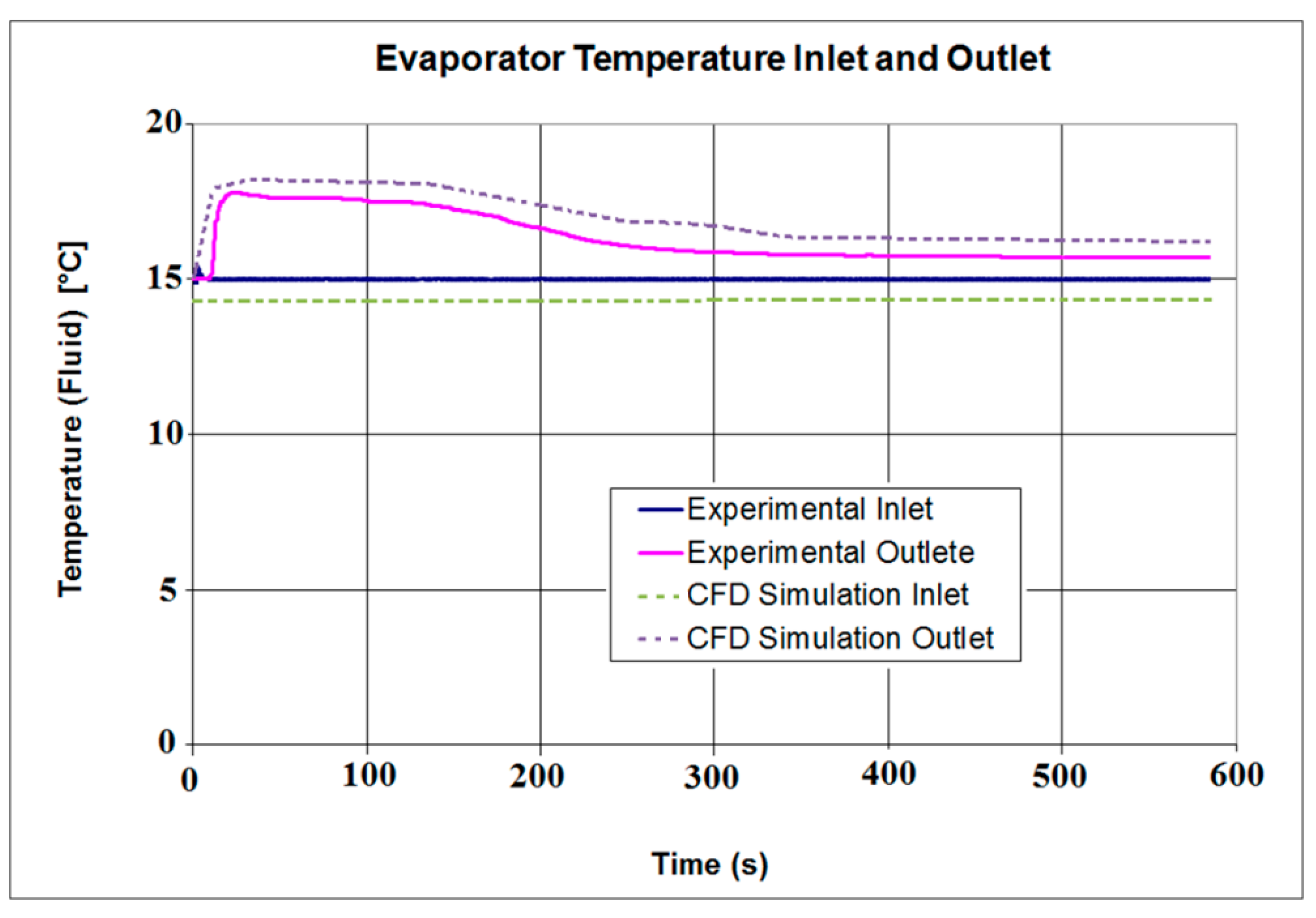
Figure 8. The refrigerant temperature in the evaporator by J. White ©2012 [10].

Figure 8. The refrigerant temperature in the evaporator by J. White ©2012 [10].

Figure 8 depicts the refrigerant temperature variation in the evaporator. It can be observed that the output temperature increases first and decreases subsequently. The experimental results from the condenser inlet and outlet refrigerant temperatures are compared to the CFD simulation inlet and outlet temperatures.

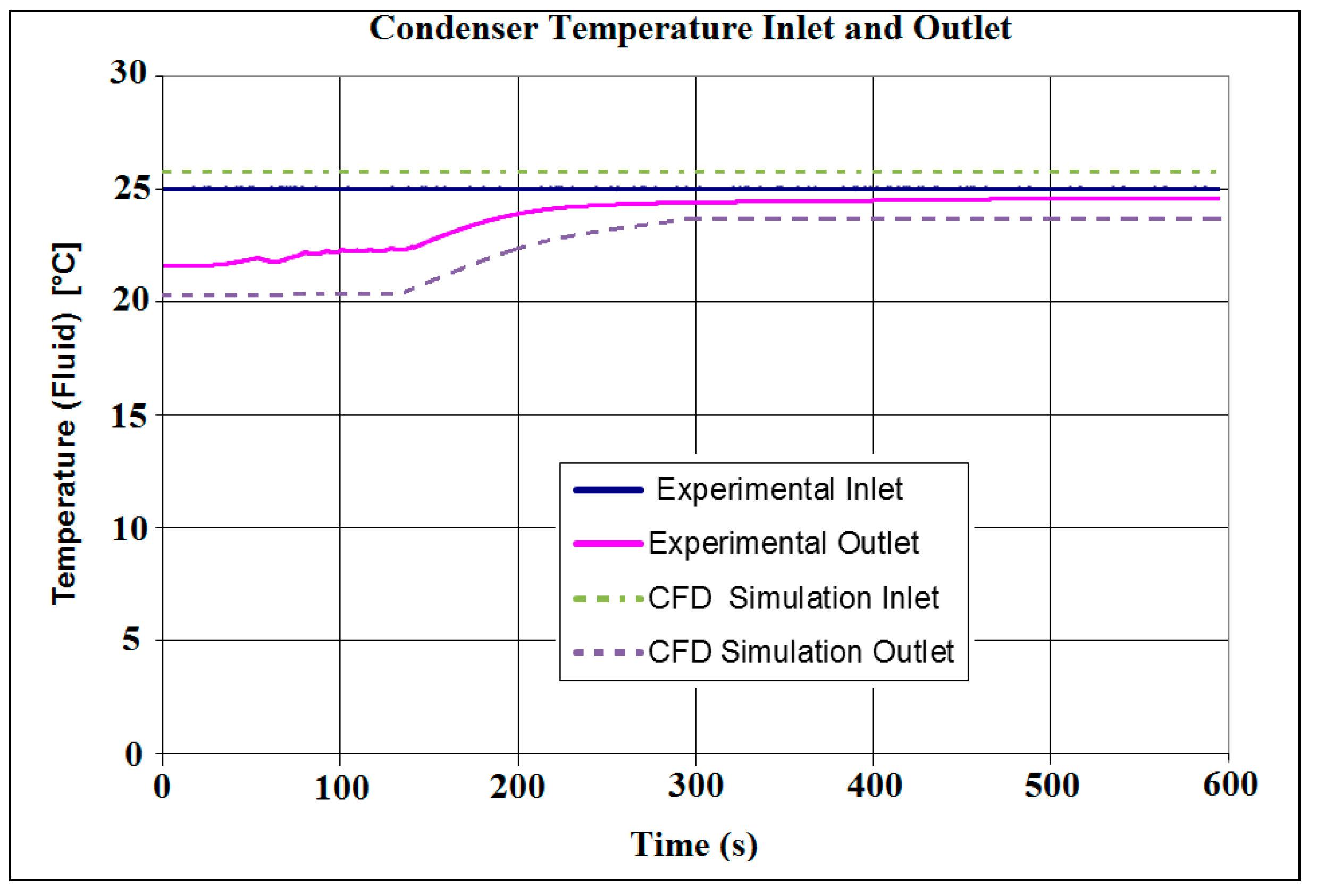
Figure 9. The refrigerant temperature in the condenser by J. White ©2012 [10].

Figure 9. The refrigerant temperature in the condenser by J. White ©2012 [10].

As seen in Figure 9 the CFD simulation results roughly agree with those of the experimental data. The inlet water to the condenser has a temperature of 25 °C, and that to the evaporator is 15 °C; these values indicate that the pressure of condenser is held at 101,325 Pa. At the inception of the adsorption-desorption period, the pressure in the condenser increases and decreases subsequently.

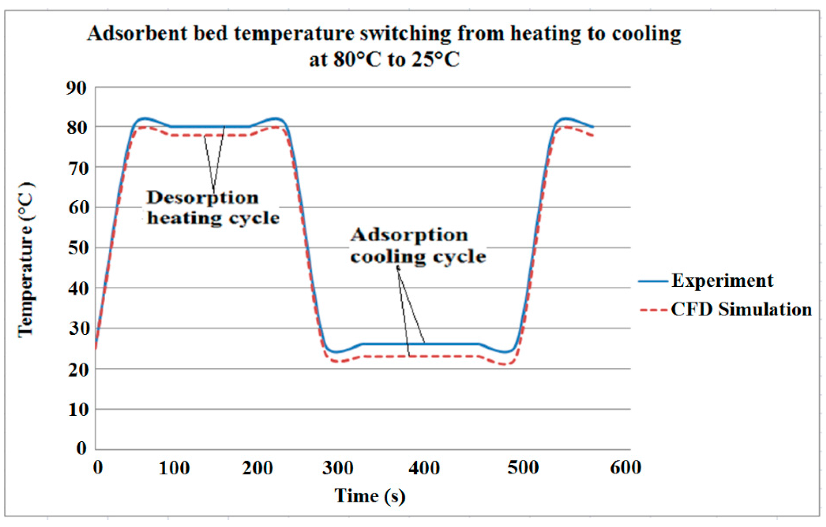
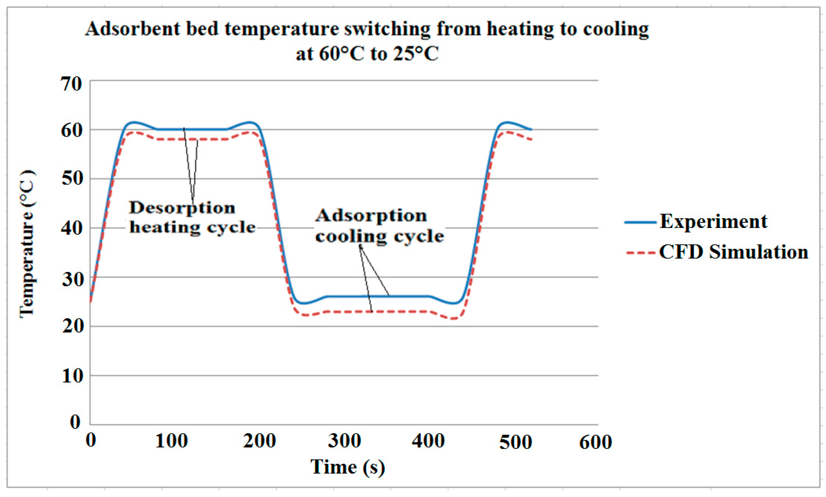
Figure 10. Comparison of the outlet temperature of the CFD simulation and the experiment data by J. White ©2012 [10].

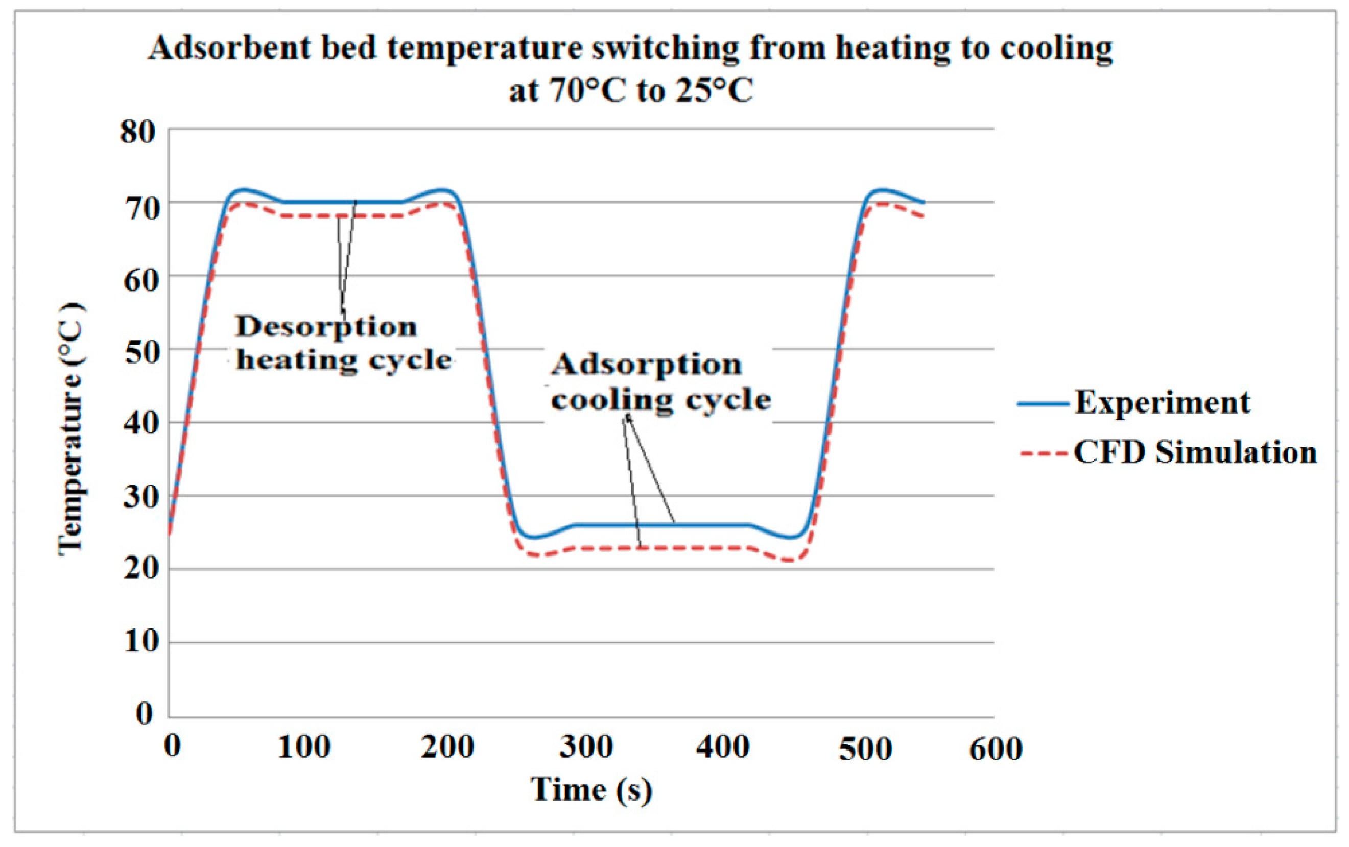
Figure 10. Comparison of the outlet temperature of the CFD simulation and the experiment data by J. White ©2012 [10].

For an adsorption cooling system, the main two operating temperatures concerned are observed in Figure 10. These are the temperature of desorption heating and the adsorption cooling temperature. It may be significant to note that the outlet temperatures of the adsorbent bed are affected by the time constant and error of the temperature sensors see Table 5.

7.2. Comparative Study

In heat exchangers, there may be different thermal heat transfer owing to the different type of heat exchanger design, creating different behavior in the heat exchanger. Therefore, CFD thermal heat transfer simulation analysis will help the design engineer to predict the behavior of the various types of heat exchanger performance. The thermal heat transfer CFD simulation performance results from a 3D CFD simulation model. A comparison of the experimental wire woven finned heat exchanger and a 3D CFD simulation model of flat fin heat exchanger as shown in Figure 11, Figure 12 and Figure 13. The heat exchanger with the capability of transferring more heat to its tip will have greater heat transfer efficiency.

7.3. Experimental Two Setup and Method

This experimental apparatus was designed to perform heat transfer analysis of heat exchangers. The adsorbent reactor bed section is removable; this is to allow changing of the different heat exchangers see Figure 11 [17,10].

Figure 11. Heat exchanger test rig.

Figure 11. Heat exchanger test rig.

Thermocouples are implanted at intervals along each fin so that temperature is known at selected points as shown in Figure 12 [10]. It is at this location that the convection coefficient will be determined. Temperature readings were examined at 60 s intervals to manage the efficiency of the different heat exchanger fins as shown in Table 6.

Figure 12. Setting up the wire woven heat transfer experiment.

Figure 12. Setting up the wire woven heat transfer experiment.

Figure 13. Setting up wire fin for heat transfer experiment.

Figure 13. Setting up wire fin for heat transfer experiment.

Table 6 shows the heat exchanger heat transfer experimental results at 85 °C.

Table 6. The stressed column indicates the values used for CFD simulation of the hot water cycle.

Test	Wire Woven Fin		Flat Fin
Time (s)	T-hot in	T-hot out	T-hot in	T-hot out
60	85	83.9	85	73.5
120	85	84.1	85	73.5
180	85	83.9	85	73.6
240	85	83.7	85	73.6
300	85	83.7	85	73.2
360	85	83.5	85	73.2
420	85	83.4	85	73.1
480	85	83.4	85	73.1
540	85	83.2	85	73.1
600	85	81.1	85	73.1
660	85	80.2	85	73.1
720	85	80.1	85	73.1
780	85	80.1	85	72.9

Table 6. The stressed column indicates the values used for CFD simulation of the hot water cycle.

Test	Wire Woven Fin		Flat Fin
Time (s)	T-hot in	T-hot out	T-hot in	T-hot out
60	85	83.9	85	73.5
120	85	84.1	85	73.5
180	85	83.9	85	73.6
240	85	83.7	85	73.6
300	85	83.7	85	73.2
360	85	83.5	85	73.2
420	85	83.4	85	73.1
480	85	83.4	85	73.1
540	85	83.2	85	73.1
600	85	81.1	85	73.1
660	85	80.2	85	73.1
720	85	80.1	85	73.1
780	85	80.1	85	72.9

The yellow bottom rows indicate the values used for CFD simulation of the hot water cycle.

7.4. Computational Fluid Dynamics Simulation of the Two Different Heat Exchangers

There are two different heat exchanger to be simulated, the flat fin heat exchanger and the wire woven heat exchanger. Both heat exchangers were simulated with the packing of silica gel porous medium, the results was compared to visualise the heat transfer performance of both.

7.5. The Physical Models

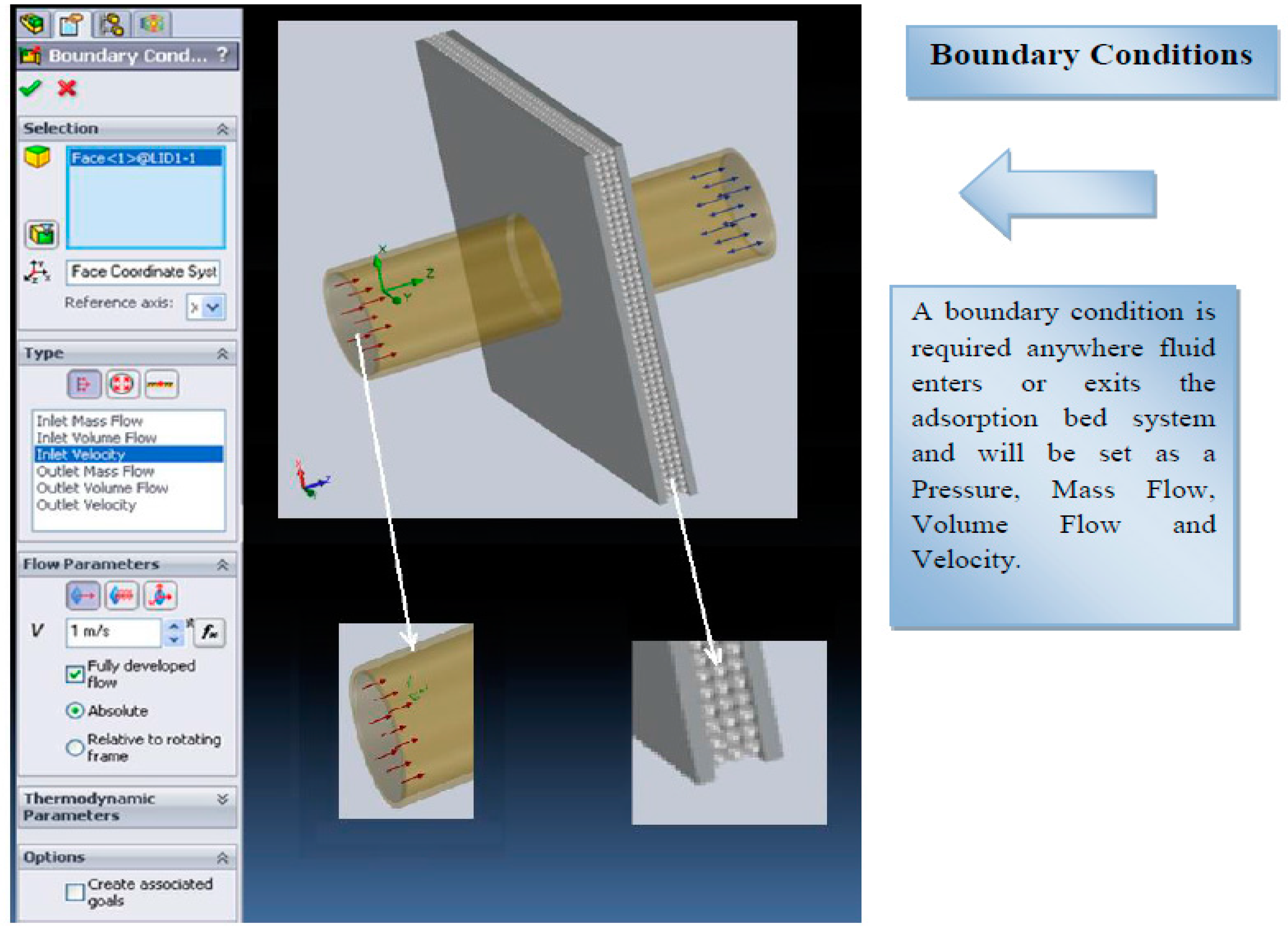
The fluid flow and thermal heat variables on the boundaries conditions of the model are:

1

Fluid flow inlet and outlet boundaries: temperature inlet, velocity inlet, temperature outlet;

2

Heat exchanger fin wall, repeating, and limit boundaries: fin wall, symmetry;

3

Internal fluid, solid;

4

Internal face boundaries: porous, fins wall, interior.

In the CFD simulation model, flow velocity was allocated to the flow inlet of the adsorbent bed; this boundary condition expresses a flow velocity at the inlet of the bed. The flow exit boundary is defined as a pressure outlet, and the outlet pressure is defined as atmospheric pressure. The adsorbent bed and packing interior are defined as boundaries. The fin wall boundaries separate the fluid zone and vapour in between the porous silica gel granules from the fin wall zones [9,10,17]. With the strength of the boundary conditions a CFD simulation can define the physical model. It was then necessary to determine how the solution will be established. This was done by setting the iteration parameters. With all boundary conditions well-defined, some additional parameters and solving schemes were selected. An initial state was assigned to the CFD simulation, which was used to help speed the merging of the calculation. The computation is an iterative process that solves the governing equations for flow and energy in each simulated cell. Depending on the difficulty of the model and the computer resources available, CFD simulation can take anywhere from minutes to days [10]. The results of the CFD simulation can be viewed and manipulated with post-processing software once the simulation has converted to a solution.

The furthermost significant portions of CFD modelling are the construction of the mesh topology. It has to be selected with enough elements to describe the methods correctly and with a degree of smoothness that allows results within a reasonable period. When an optimal density has been found, refining this will increase the model size without displaying more flow detail [10,11,12,13,14,15,16,17]. Once it is coarsened the mesh will obscure possibly essential parts of the flow detail. The mesh determines a large part of creating an acceptable simulation; see Figure 14 which illustrate the stages followed to achieve the results that were discussed in this section.

Figure 14. Porous adsorbent CFD simulation methodology.

Figure 14. Porous adsorbent CFD simulation methodology.

Define the Engineering Goal

Engineering goals are the parameters which you need for the CFD simulation. Setting goals is one way of assigning to the CFD Simulation what you are trying to get out of the investigation as well as a way to reduce the time CFD Flow Simulation needs to reach a solution.

Goals can be set all through the entire domain (Global Goals), with some volumes (volume Goals), in a nominated surface area (Surface Goals), or at a given (Point Goals).

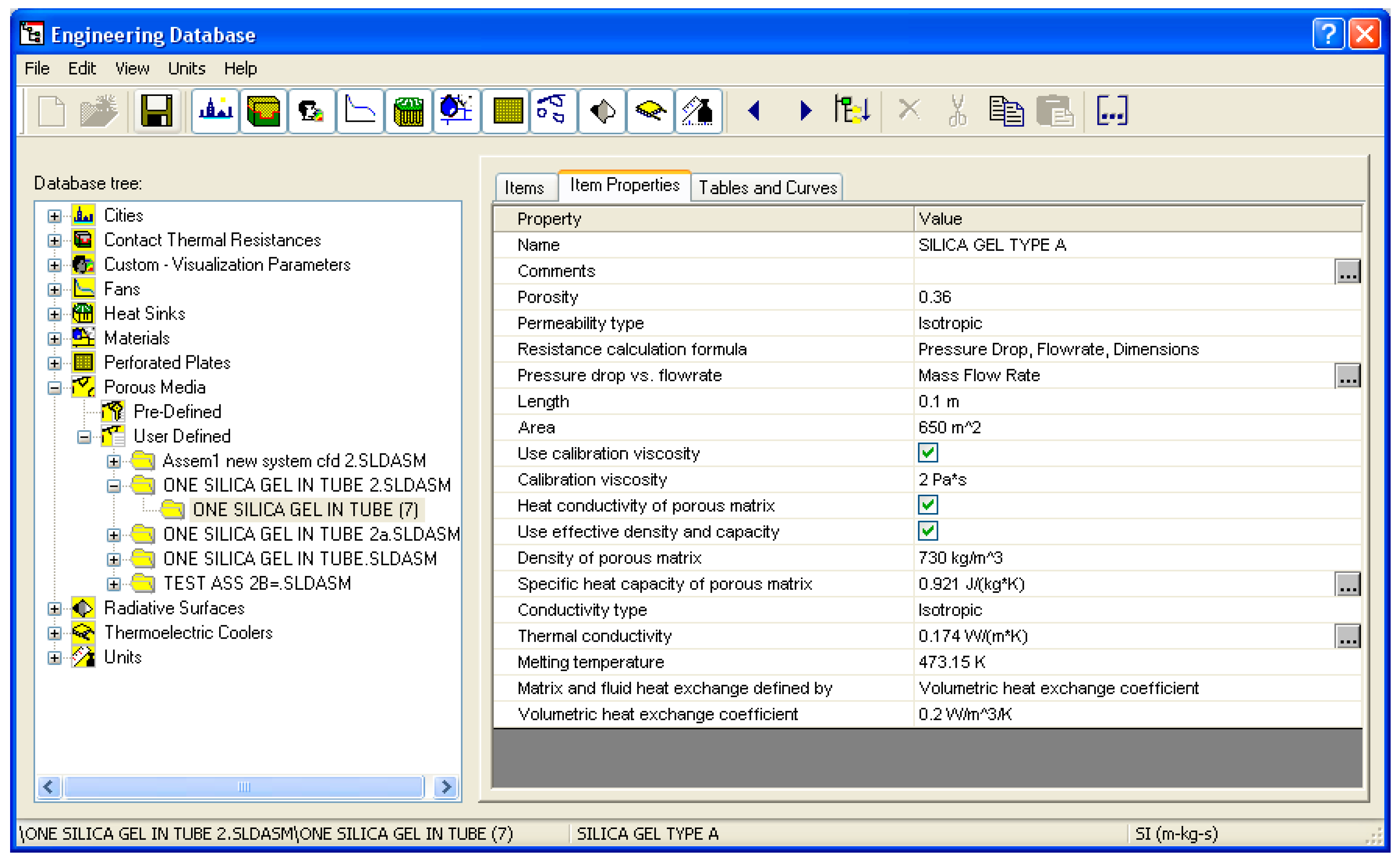
7.6. Creating the Silica Gel Porous Medium

To generate a porous medium for the adsorbent bed, first specify the porous medium’s properties (porosity, permeability type, etc.) in the Engineering Database and then apply the porous medium to the spheres in the packed bed assembly. The data shown in Figure 15 were those specified in this simulation.

Figure 15. Creating the silica gel porous medium in CFD Cosmos flow simulation.

Figure 15. Creating the silica gel porous medium in CFD Cosmos flow simulation.

For the porous medium simulation method, the CFD model has a mass of cells representing the fluid inlet [15,16,17]. This is followed by the porous adsorbent units that are used to model fluid flow through porous adsorbent [4,10,15]. Full flow field predictions are possible with the porous adsorbent simulation method because the equations describe the resistance of the porous adsorbent to flow:

$$\frac{\Delta P}{L}=-\alpha U_S^2-\beta U_S$$

(8)

Here the coefficient values α and β are allocated temperature-dependent values that describe the performance of a porous adsorbent. High values of α and β preclude flow at right angles to the porous adsorbent. Upstream and downstream of the water vapour flow field are solved using the usual Reynolds-averaged Navier-Stokes methodology.

7.7. Thermophysical Properties

Once the model was established, boundary conditions were assigned to each section of the model and were used to simulate the actual conditions set by the adsorption cooling system. Examples of common boundary conditions include velocity inlet, pressure inlet, pressure outlet, and temperature profile as seen in Table 7, Table 8 and Table 9 [10].

Table 7. Thermophysical properties of copper tube.

Material	Water
Density, ρ (kg/m3)	1000
Specific Heat Capacity CP (J/kg·K)	4200
Thermal Conductivity, K (W/m·K)	0.61
Dynamic Viscosity, µ (kg/ms) × 10−3	0.96172

Table 7. Thermophysical properties of copper tube.

Material	Water
Density, ρ (kg/m3)	1000
Specific Heat Capacity CP (J/kg·K)	4200
Thermal Conductivity, K (W/m·K)	0.61
Dynamic Viscosity, µ (kg/ms) × 10−3	0.96172

Table 8. Thermo-physical properties of silica gel.

Thermophysical Properties of Silica Gel	Type A
Specific Surface Area (m2/g)	650
Porous Volume (mL/g)	0.36
Average Pore Diameter (A)	22
Apparent Density (kg/m3)	730
pH Value	5.0
Water Content (wt.%)	<2.0
Specific Heat Capacity (KJ/kg·K)	0.921
Thermal Conductivity (W/m·K)	0.174
Mesh Size	10–40

Table 8. Thermo-physical properties of silica gel.

Thermophysical Properties of Silica Gel	Type A
Specific Surface Area (m2/g)	650
Porous Volume (mL/g)	0.36
Average Pore Diameter (A)	22
Apparent Density (kg/m3)	730
pH Value	5.0
Water Content (wt.%)	<2.0
Specific Heat Capacity (KJ/kg·K)	0.921
Thermal Conductivity (W/m·K)	0.174
Mesh Size	10–40

Table 9. Thermo-physical properties of alumina fins.

Property	Value	Units
Elastic Modulus	1.1e+11	N/m2
Poissons Ratio	0.37	N/A
Shear Modulus	4e+10	N/m2
Density	8900	kg/m3
Tensile Strength	394,380,000	N/m2
Compressive Strength in X		N/m2
Yield Strength	258,646,000	N/m2
Thermal Expansion Coefficient	2.4e−5	/K
Thermal Conductivity	390	W/(m·k)
Specific Heat	390	J/(kg·K)
Material Damping Ratio		N/A

Table 9. Thermo-physical properties of alumina fins.

Property	Value	Units
Elastic Modulus	1.1e+11	N/m2
Poissons Ratio	0.37	N/A
Shear Modulus	4e+10	N/m2
Density	8900	kg/m3
Tensile Strength	394,380,000	N/m2
Compressive Strength in X		N/m2
Yield Strength	258,646,000	N/m2
Thermal Expansion Coefficient	2.4e−5	/K
Thermal Conductivity	390	W/(m·k)
Specific Heat	390	J/(kg·K)
Material Damping Ratio		N/A

7.8. Surface Area and Volume of Flat Fin Results Generated by CFD

For most finned heat exchangers, the materials determine transfers, thermal conductivity and the structures surface area to volume ratio. As mentioned, before increasing, the surface of a heat exchanger will also increase the heat transfer of the heat exchangers. To investigate the surface area to volume ratio and heat transfer of heat exchangers, two different types of heat exchangers were selected and compared.

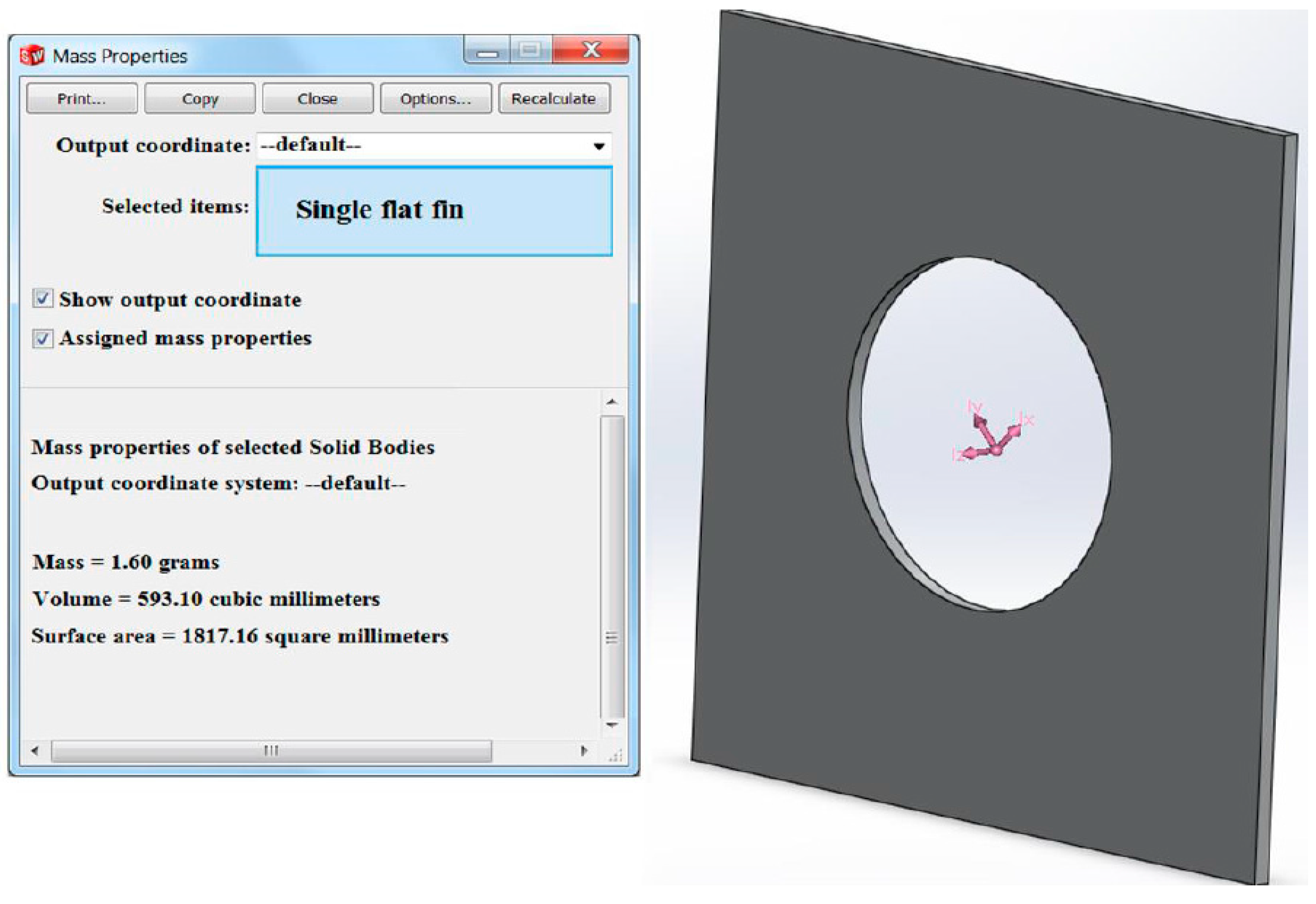
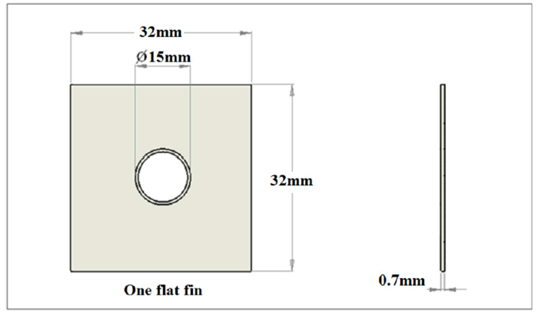
The length and the height of the flat aluminium heat exchanger fin are 32 mm and 32 mm, respectively, as shown in Figure 16 and Figure 17.

Figure 16. Drawing dimensions for Aluminium flat finned heat exchanger used to generate volume and surface area of fin.

Figure 16. Drawing dimensions for Aluminium flat finned heat exchanger used to generate volume and surface area of fin.

Figure 17. Single flat fin volume and surface area generated by assigning mass properties to 3D CAD model.

Figure 17. Single flat fin volume and surface area generated by assigning mass properties to 3D CAD model.

A mesh was created to focus on silica gel contact points and silica gel heat exchanger wall contact points. The porous silica gel geometry in CFD flow simulation was also prepared to match the outcomes of CFD codes. When real contact points are created, both surfaces that are contacting have one common node [10,15,16,17]. In surface mesh formation, this can be defined and does not pose any problems. The 3D mesh was created reasonably easily by the inclusion of some nodes on the interactive surfaces. In the laminar flow case, the solution parameters were adjusted to get a converging solution please see Figure 18 [10,15,16,17].

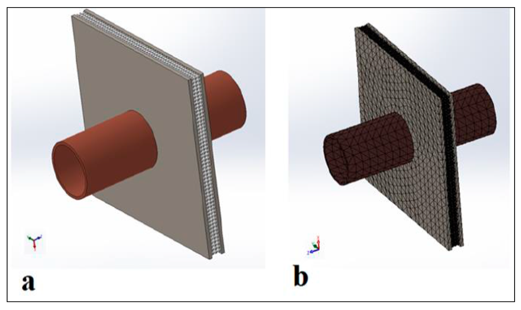
Figure 18. Aluminium flat plate finned heat exchanger (a) and (b) presents the flat fin mesh.

Figure 18. Aluminium flat plate finned heat exchanger (a) and (b) presents the flat fin mesh.

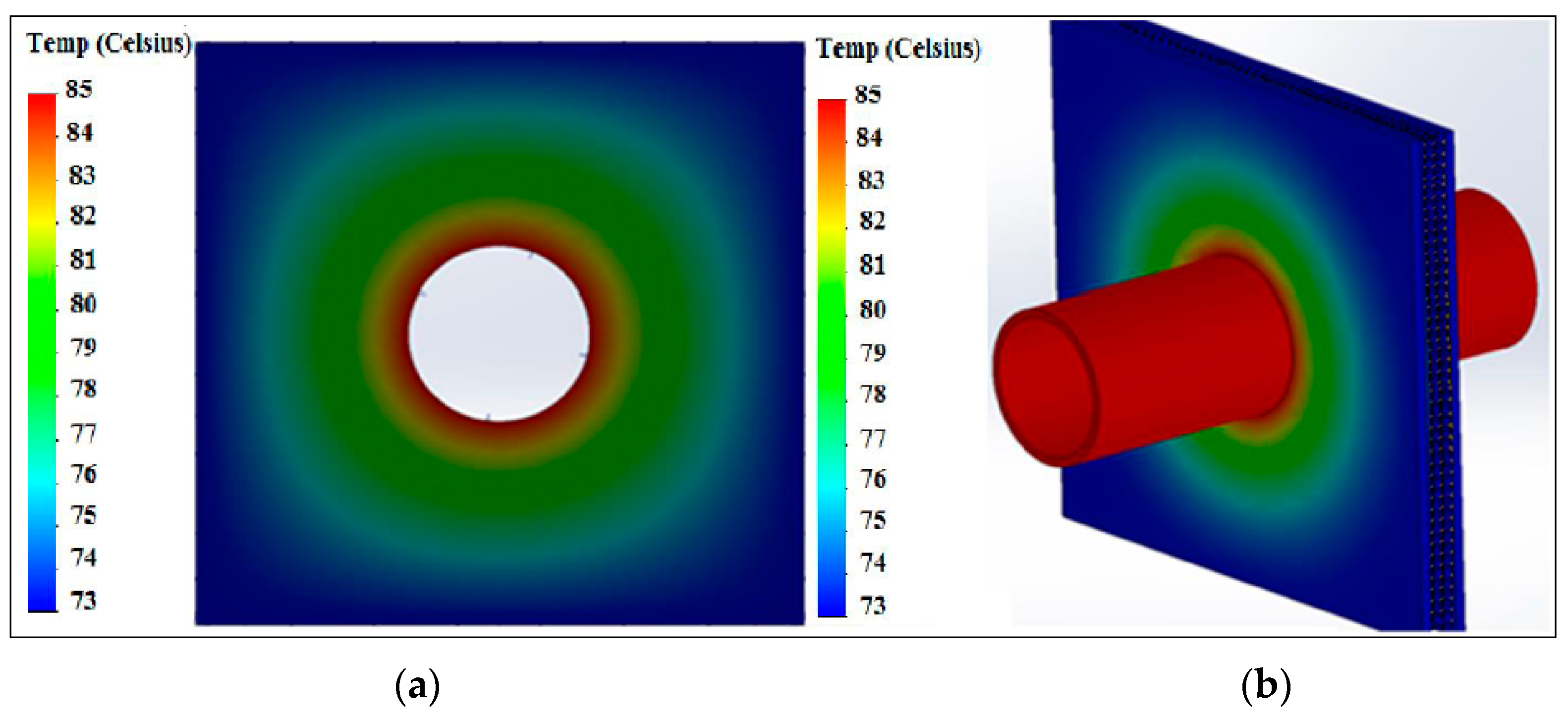
The fin root temperature as seen in Figure 19a,b was set at 85 °C, and the model was run until the solution approached the steady state behavior after 750 s. The fin root temperature changed from 85 °C to 73 °C as the heat was conducted to the top edge of the fin. This shows a reduction in temperature of the Aluminum flat plate fin by 12 °C. This reduction in temperature is partly due to the heat transfer from the Aluminum fin to porous adsorbent, see Figure 19 and Figure 20.

Figure 19. The contour thermal heat transfer temperature of the flat finned heat exchanger (a); The Centre of the fin is 85 °C and the fin edge is 73 °C (b).

Figure 19. The contour thermal heat transfer temperature of the flat finned heat exchanger (a); The Centre of the fin is 85 °C and the fin edge is 73 °C (b).

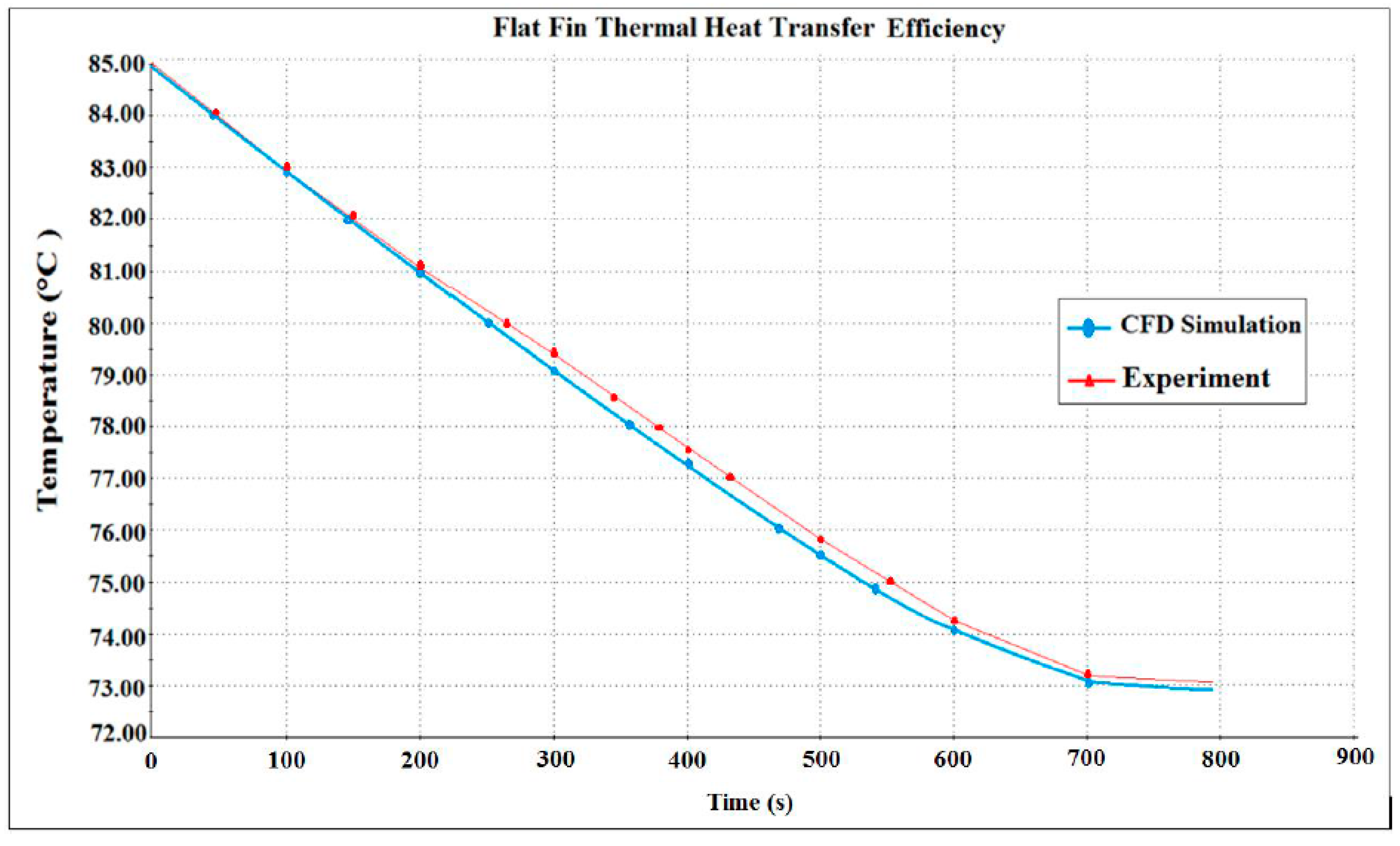
Figure 20. Changes of heat transfer efficiency over time.

Figure 20. Changes of heat transfer efficiency over time.

Temperature distribution in Figure 20 presents the temperature provided lengthwise of the rectangular heat exchanger fin. A higher gradient can be detected near the base of the heat exchanger fin due to the temperature difference between the fin surface and the surrounding porous adsorbents covering the fins.

7.9. Surface Area and Volume of Wire Fin Results Generated by CFD

In this section, the surface area and volume of the two different heat exchanger will be simulated using the experimental input data obtained so as to be able to visualize the CFD simulated heat transfer root contours.

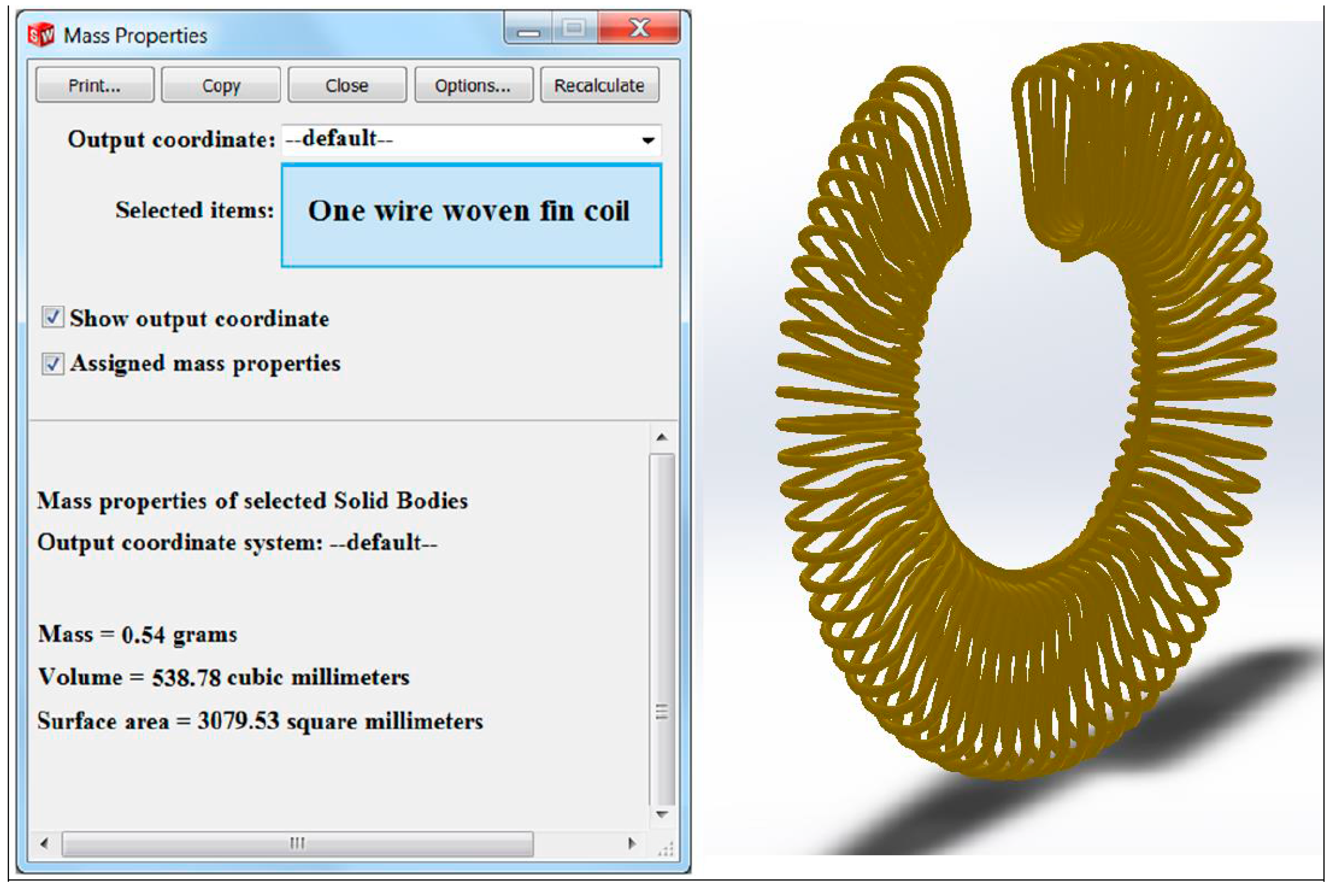
7.10. Wire Finned Heat Exchanger Surface Area and Volume

The surface area of one copper wire woven fin coil is 3079.53 square millimetres. This comprises 0.7 mm copper wire 1400 mm in length woven coiled into 70 loops as shown in Figure 21 and Figure 22.

Figure 21. Drawing dimension for copper wire woven finned heat exchanger used to generate volume and surface area of the fin.

Figure 21. Drawing dimension for copper wire woven finned heat exchanger used to generate volume and surface area of the fin.

Figure 22. One wire woven fin volume and surface area generated 3D CAD model.

Figure 22. One wire woven fin volume and surface area generated 3D CAD model.

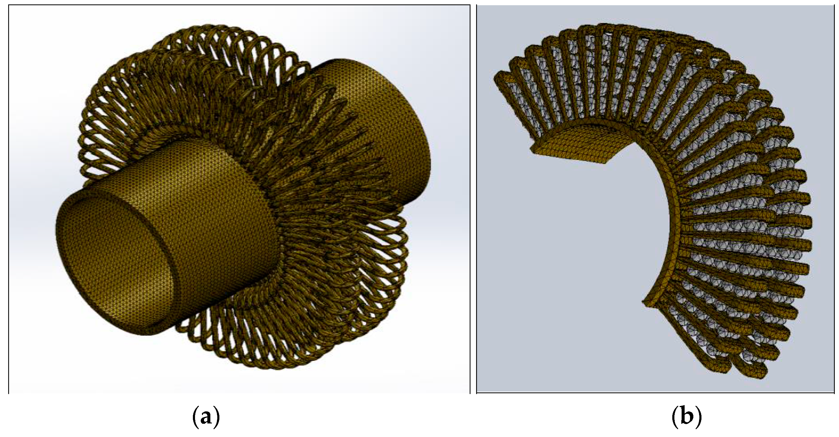
7.11. The Wire Woven Fin Adsorbent Bed

The method used to carry out the simulation of this type of adsorbent bed is the same as that described above. To reduce the time for CFD simulation, small geometries of the copper fin with an adsorbent packed between one pitch were used as a model for the CFD simulation see Figure 23.

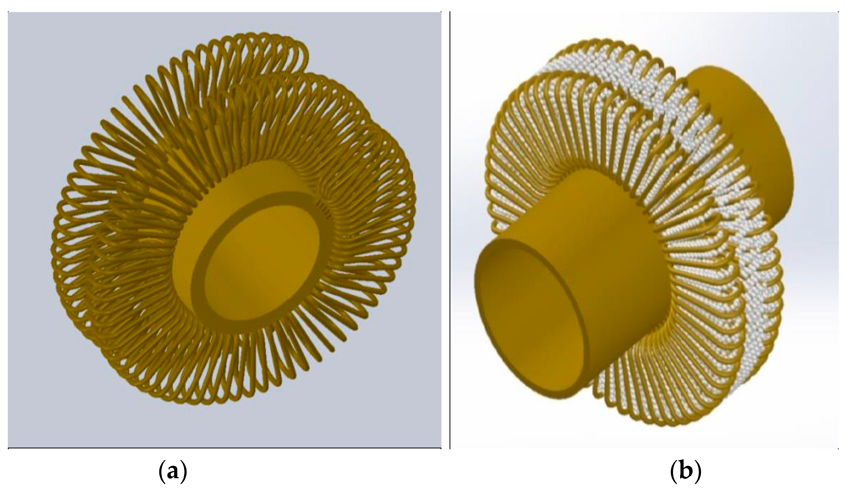
Figure 23. 3D model of the wire fin without silica gel and with silica gel. (a) The wire fin has no silica gel packing as can be seen from the 3D CAD model; (b) The heat exchanger has porous adsorbent added to it as can be seen in the 3D model.

Figure 23. 3D model of the wire fin without silica gel and with silica gel. (a) The wire fin has no silica gel packing as can be seen from the 3D CAD model; (b) The heat exchanger has porous adsorbent added to it as can be seen in the 3D model.

In Figure 23a the wire fin has no silica gel packing. In Figure 23b the heat exchanger has porous adsorbent added to it. Both Figure 23a,b was simulated as can be seen in Figure 24.

7.12. One Pitch of Woven Wire Finned Heat Exchanger Mesh

The mesh for the one pitch of woven wire finned heat exchanger contains 187,365 nodes and 84,383 elements; see Figure 24. The CFD program creates the mesh based on the input parameters enter into the user-defined function menu.

Figure 24. CFD representations showing a mesh detail of the wire woven fin pack with the adsorbent. (a) shows the CFD simulation meshes must have a sufficient number of points in the internal of the computational domain to describe the physical domain correctly; (b) shows an appropriate number of points need to be specified on the boundary conditions to characterise it accurately.

Figure 24. CFD representations showing a mesh detail of the wire woven fin pack with the adsorbent. (a) shows the CFD simulation meshes must have a sufficient number of points in the internal of the computational domain to describe the physical domain correctly; (b) shows an appropriate number of points need to be specified on the boundary conditions to characterise it accurately.

In Figure 24 the CFD mesh quality can be identified through two main factors. The first factor is that the CFD simulation meshes must have a sufficient number of points in the internal of the computational domain to describe the physical domain correctly (Figure 24a). The second factor requirement for CFD mesh quality is that an appropriate number of points need to be specified on the boundary conditions to characterise it accurately (Figure 24b). This needs some boundary points to adapt according to the model surface geometry.

7.13. One Pitch of Wire Woven Finned Heat Exchanger with Adsorbent Packing

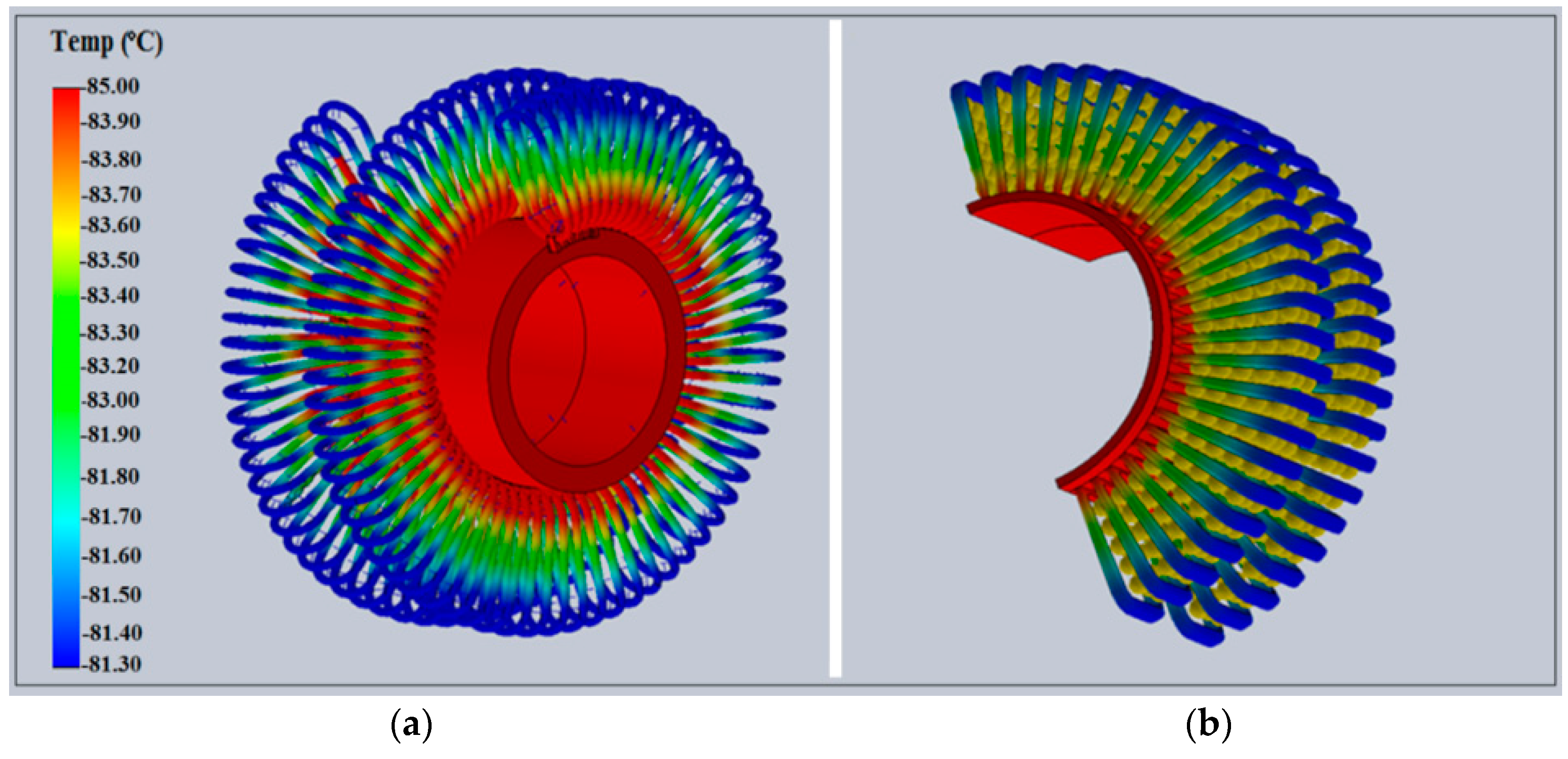
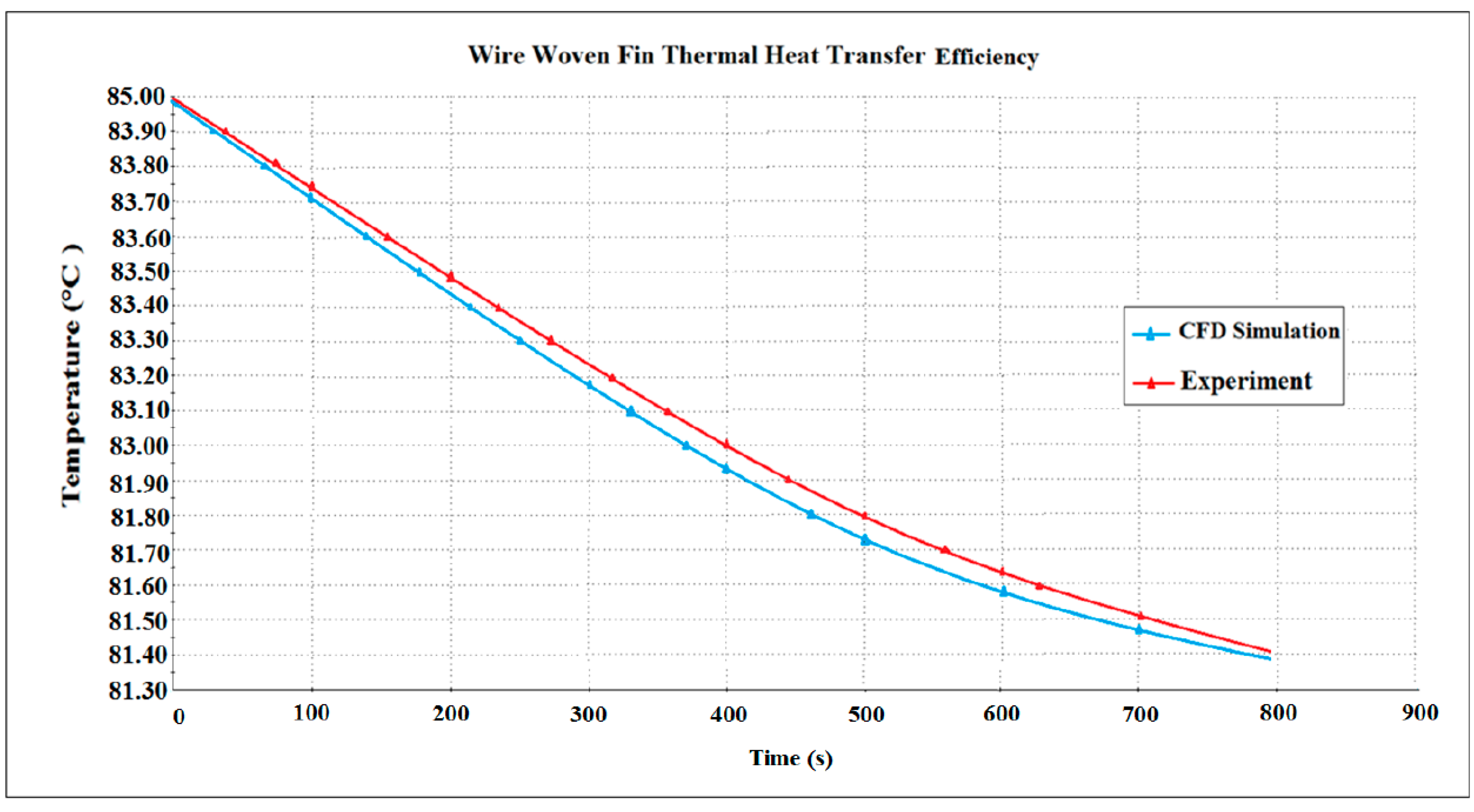
Figure 25 and Figure 26 present the temperature supplied along the length of the woven wire heat exchanger. A higher slope can be observed near the base of the fin due to the temperature change between the fin surface and the surrounding porous adsorbents covering the fins.

Figure 25. The heat transfer efficiency of the wire woven heat exchanger contour temperature is at 85 °C and the fin tip temperature is at 81 °C. (a) and (b) are cut in two to speed up the simulation time.

Figure 25. The heat transfer efficiency of the wire woven heat exchanger contour temperature is at 85 °C and the fin tip temperature is at 81 °C. (a) and (b) are cut in two to speed up the simulation time.

Figure 26. Variations of heat transfer over time.

Figure 26. Variations of heat transfer over time.

8. Validation of CFD Simulation Model

The CFD simulation model was validated with the help of experimental data obtained from tests conducted on the test rig. The detailed view of the wire fins adsorption test rig is shown in Figure 26. Measurement results were used as input parameters for the CFD simulation model of the cooling system that was developed to evaluate the performance of this system at a different temperature. In the validation of the model of the proposed wire woven fin adsorbent cooling system, the test was run so as to accumulate the relevant data for the simulation. The average error between CFD simulation and the experimental data was determined as:

$$\begin{array}{l}\epsilon =\frac{1}{N} \sum \frac{|CalculatedValue-MeasuredValue|}{MeasuredValue}\\ \text{Or in percentage}\\ \epsilon \left[\%\right]=\frac{1}{N} \sum \frac{|CalculatedValue-MeasuredValue|}{MeasuredValue}\times 100\end{array}$$

(9)

where ε is the average error, N is the number of samples.

The system temperatures are an important variable input that influences the performance of the adsorption cooling system. The change occurring at the different temperature during the test was used to study its effect on the cooling capacity of the system. The total cooling adsorption cooling and heating desorption temperature both from the test and simulation data of the system were used as a dependent variable and drawn against the inlet temperature as the independent variable. Figure 27 and Figure 28 show the experimental validation of the CFD simulated cooling and heating capacities under varying inlet temperature.

Figure 27. Comparison of the outlet temperature of the CFD simulation and the experiment data by J. White ©2012 [10].

Figure 27. Comparison of the outlet temperature of the CFD simulation and the experiment data by J. White ©2012 [10].

Figure 28. Comparison of the outlet temperature of the CFD simulation and the experiment data by J. White ©2012 [10].

Figure 28. Comparison of the outlet temperature of the CFD simulation and the experiment data by J. White ©2012 [10].

The solid lines in all figures show the experimental outlet cooling and heating temperature variation over time and dots represent the CFD cooling temperature variation over time. It is clear from these figures that both simulation and test results show the same trend, i.e., the cooling temperature was proportional. An agreement of validation was observed for most of the data error analysis, which showed a deviation of 6% and 3.4% respectively.

9. Conclusions

The simulation code has been tested for stability in computation and can achieve CFD simulation of the wire woven fin heat exchanger and the different components of the adsorption cooling system. The comparison of CFD simulated results and experimental data proves that the CFD model is a reliable tool. With this simulation tool, the time and cost of designing an adsorption cooling system could be reduced by the design of an adsorbent bed system as it provides a valuable prediction for component performances. With minor modifications, it can be extended for use with other configurations of the multi-bed system.