
Validation of the GPU-Accelerated CFD Solver ELBE for Free Surface Flow Problems in Civil and Environmental Engineering

Abstract
:1. Introduction
2. The elbe Code
2.1. Lattice Boltzmann Method
2.2. Free Surface Model
2.3. Fluid-Structure Interaction
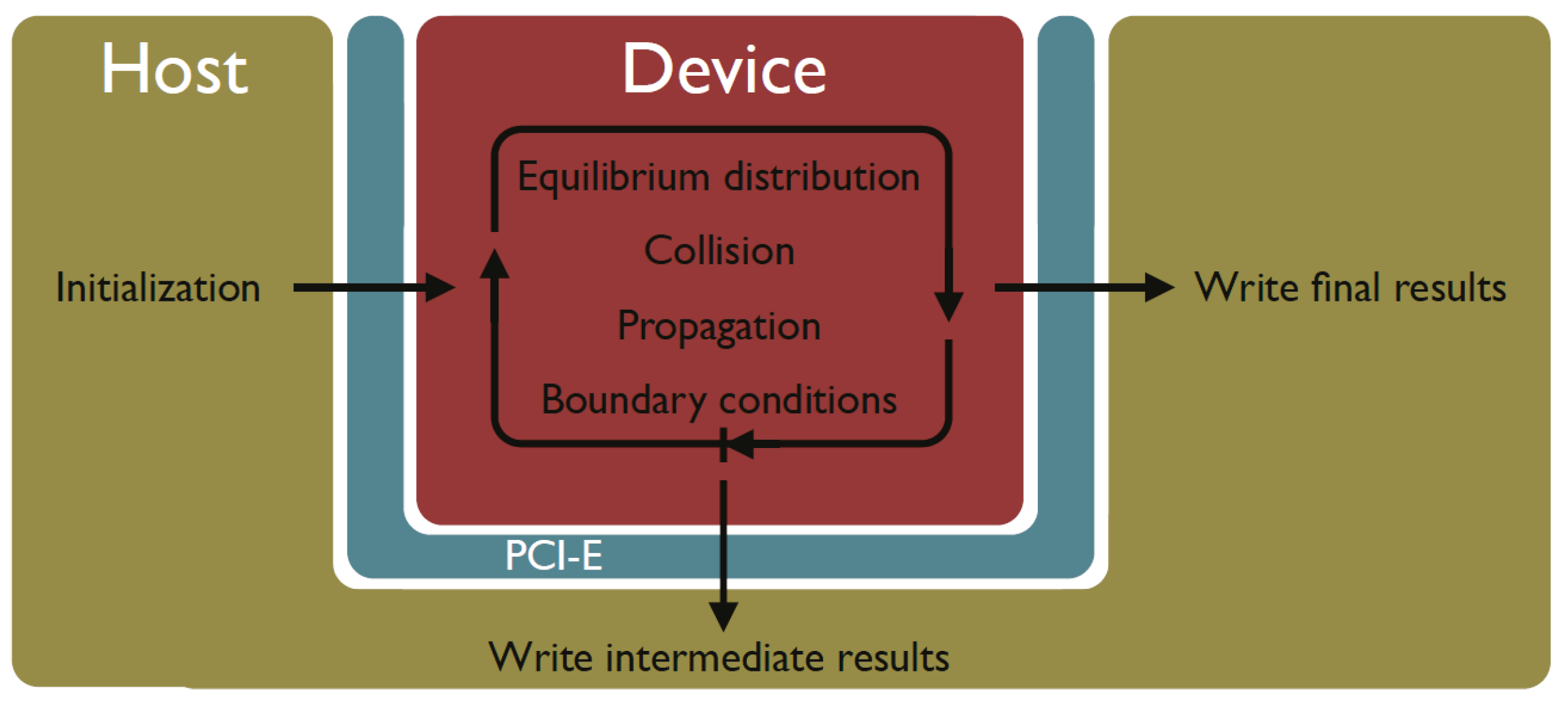
2.4. Implementation


2.5. Summary
3. Wave Propagation and Inundation Modeling
3.1. Wave Propagation in Shallow Waters
3.1.1. Validation with Catalina Benchmark Problems
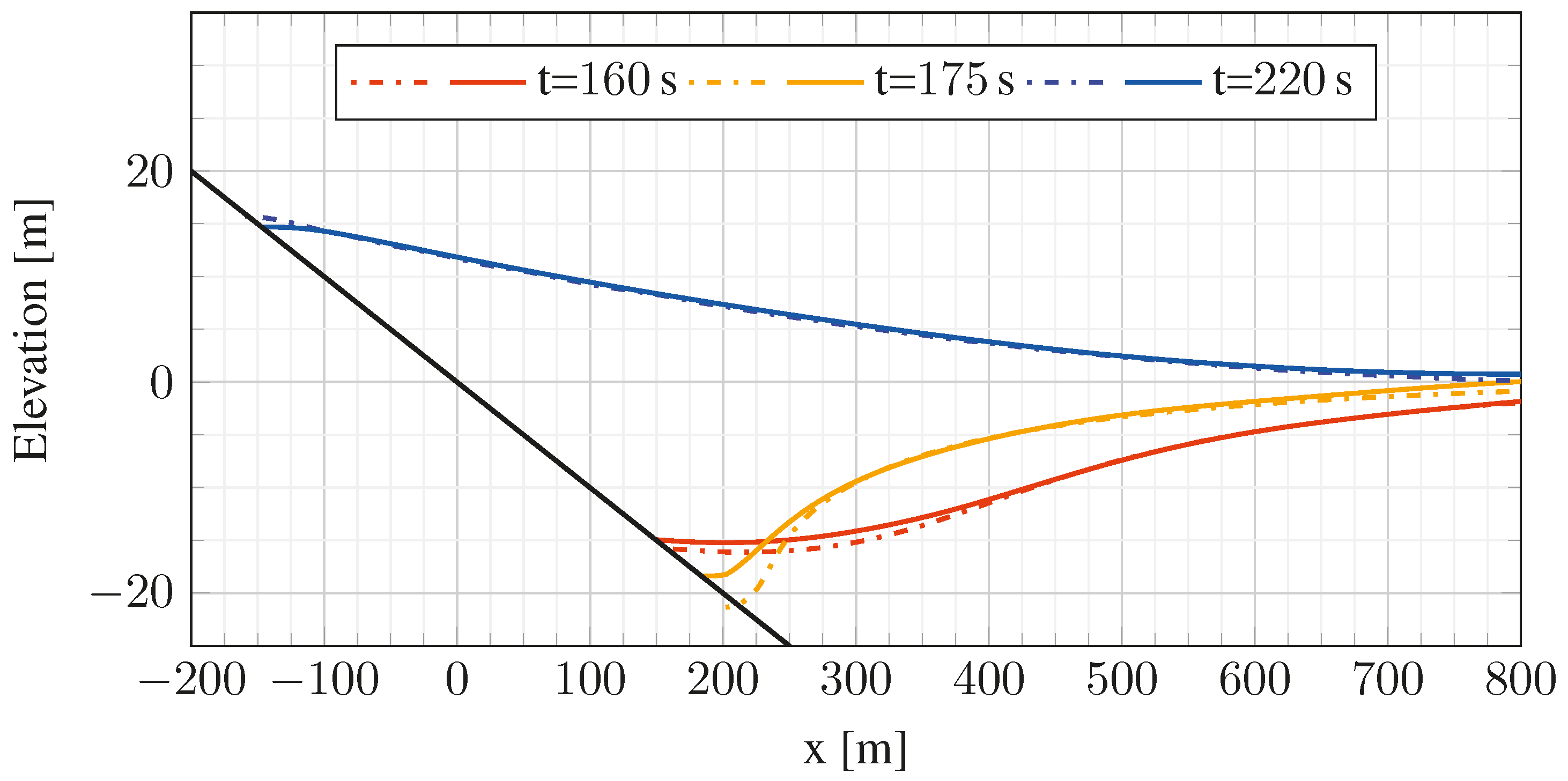
A. 2D Tsunami Runup over a Plane Beach

B. Tsunami Runup over a Complex 3D Natural Beach


C. Performance Considerations

| Solver | Grid | Δx | Δt | Time steps | Duration | NUP | Core-h | MNUPS | KNUPS/Core |
|---|---|---|---|---|---|---|---|---|---|
| FUNWAVE | 892 × 244 | 1.4 cm | 5 ms | 10,000 | 42 min | 2.1 × 10⁹ | 11 h | 0.86 | 54 |
| LBM | 512 × 256 | 1.4 cm | 0.25 ms | 200,000 | 4 min | 2.6 × 10¹⁰ | 30 h | 105 | 234 |
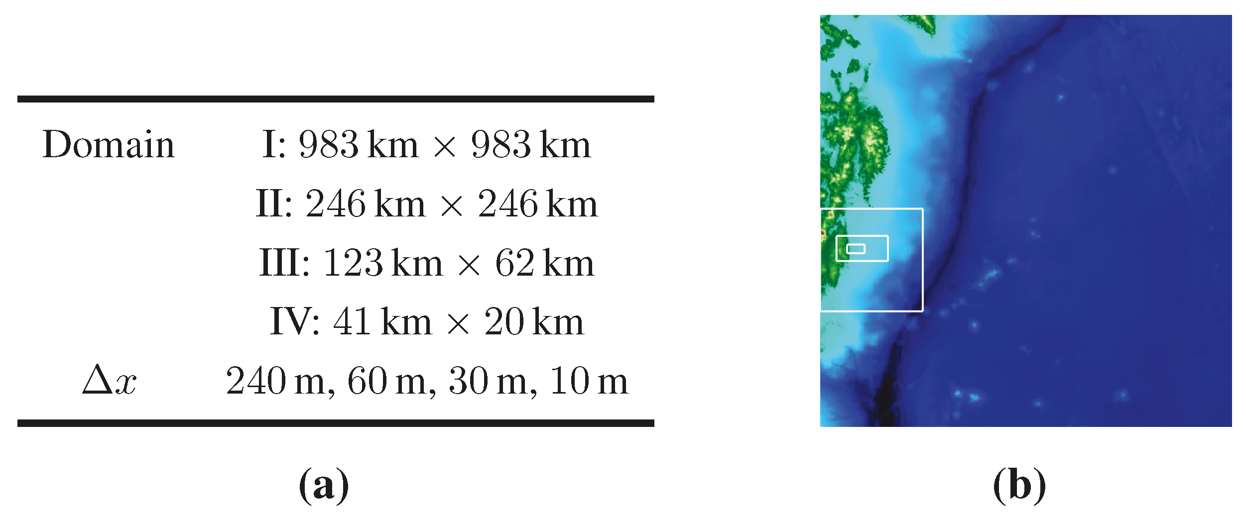
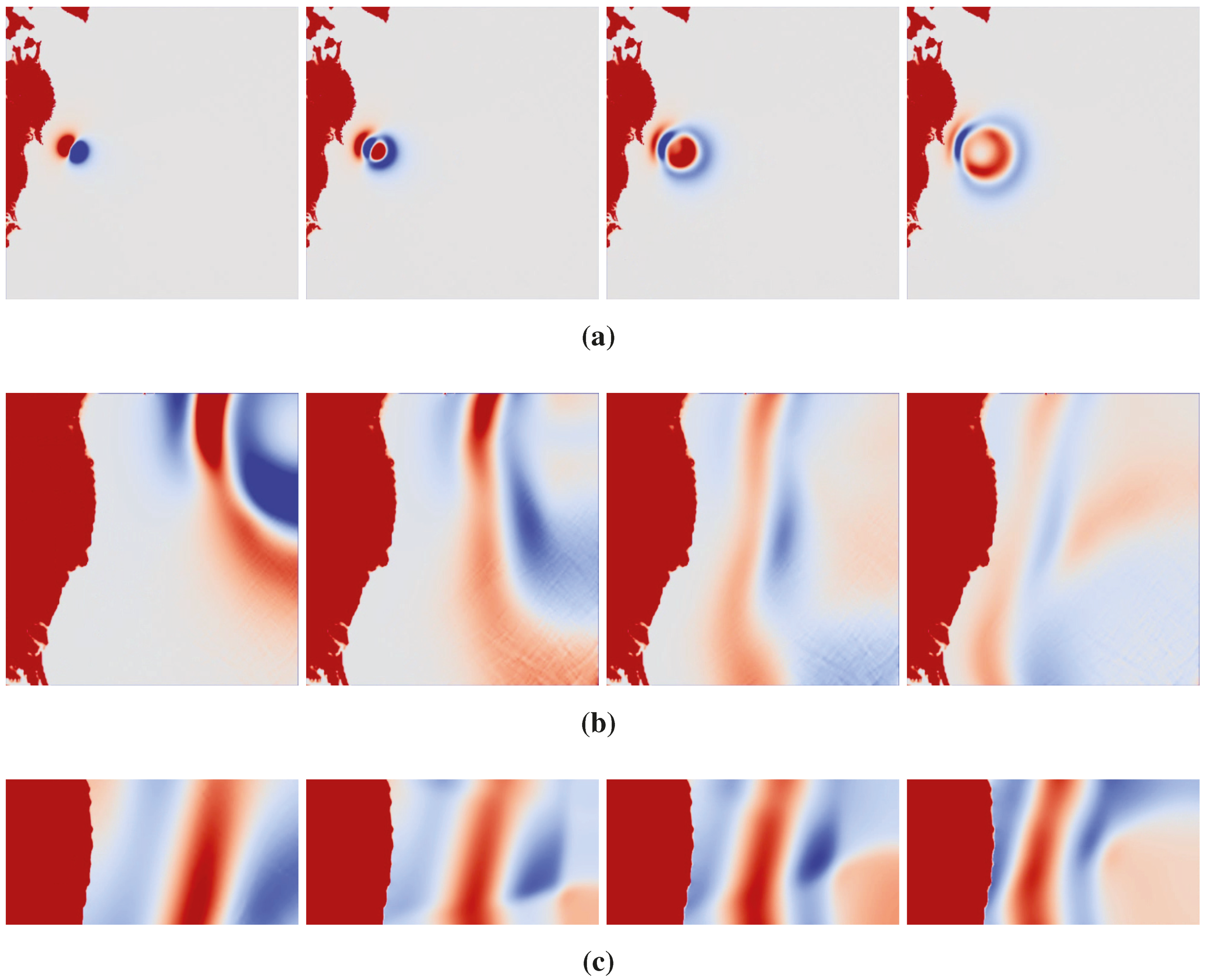
3.1.2. Tohoku Tsunami

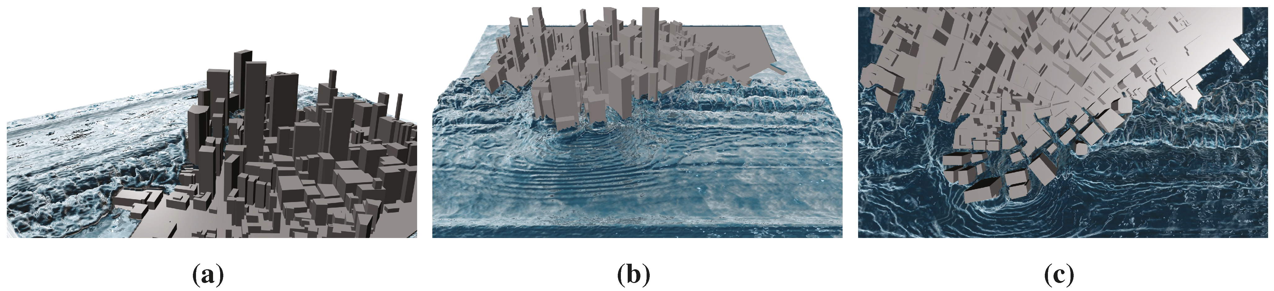
3.2. Near-Field Wave Impact

4. Debris Flow: Coupling to a Physics Engine
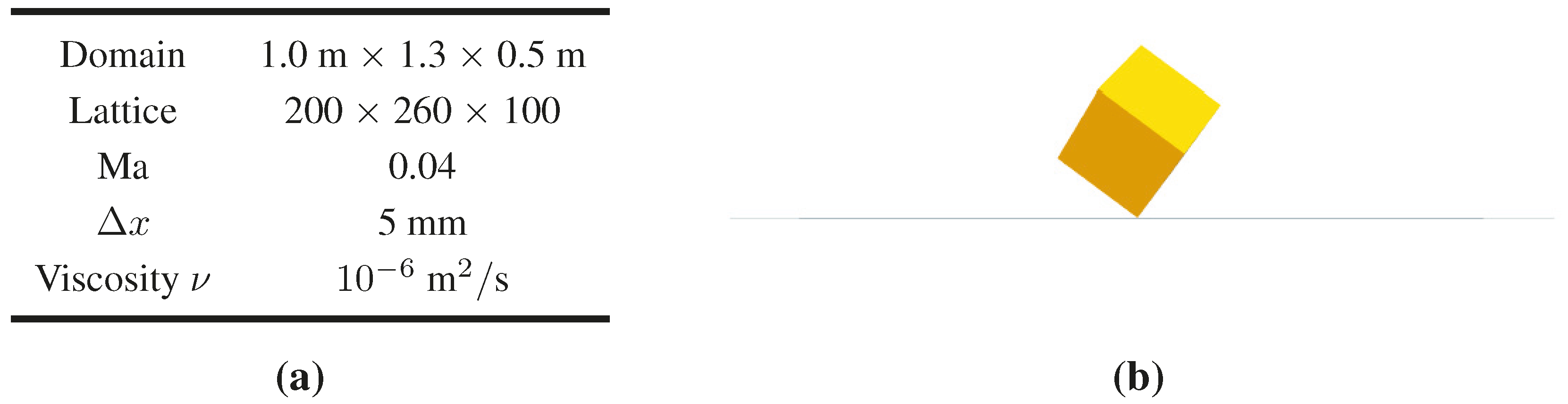
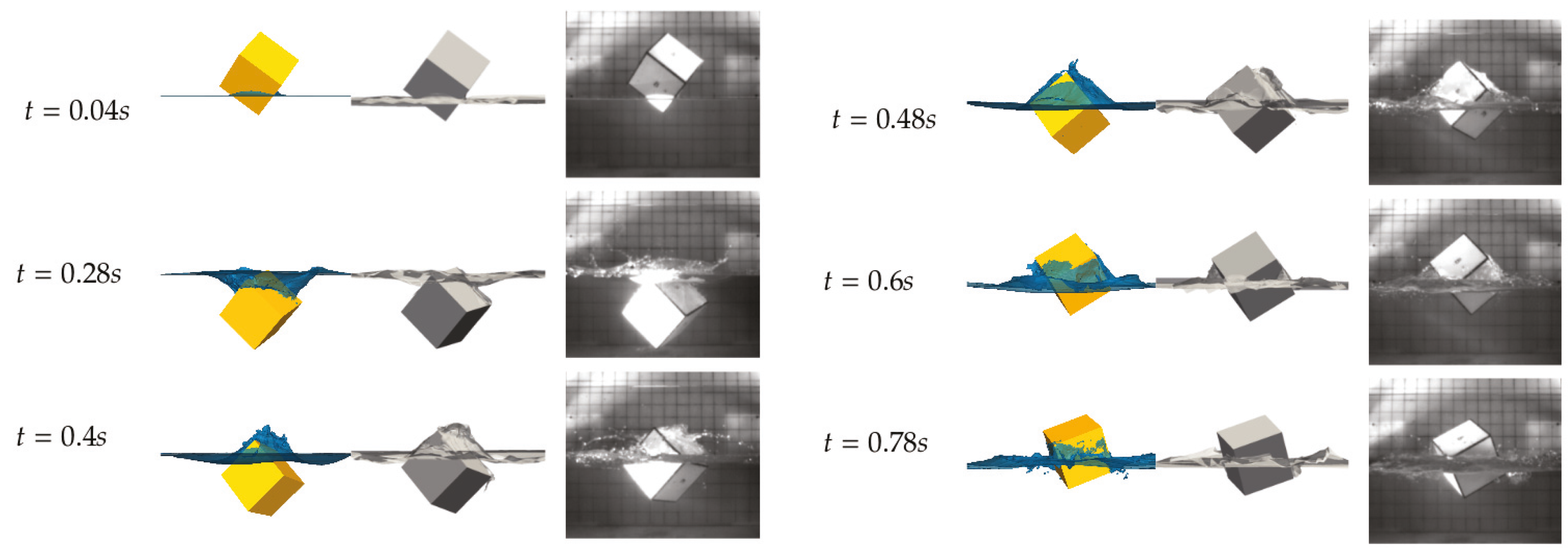
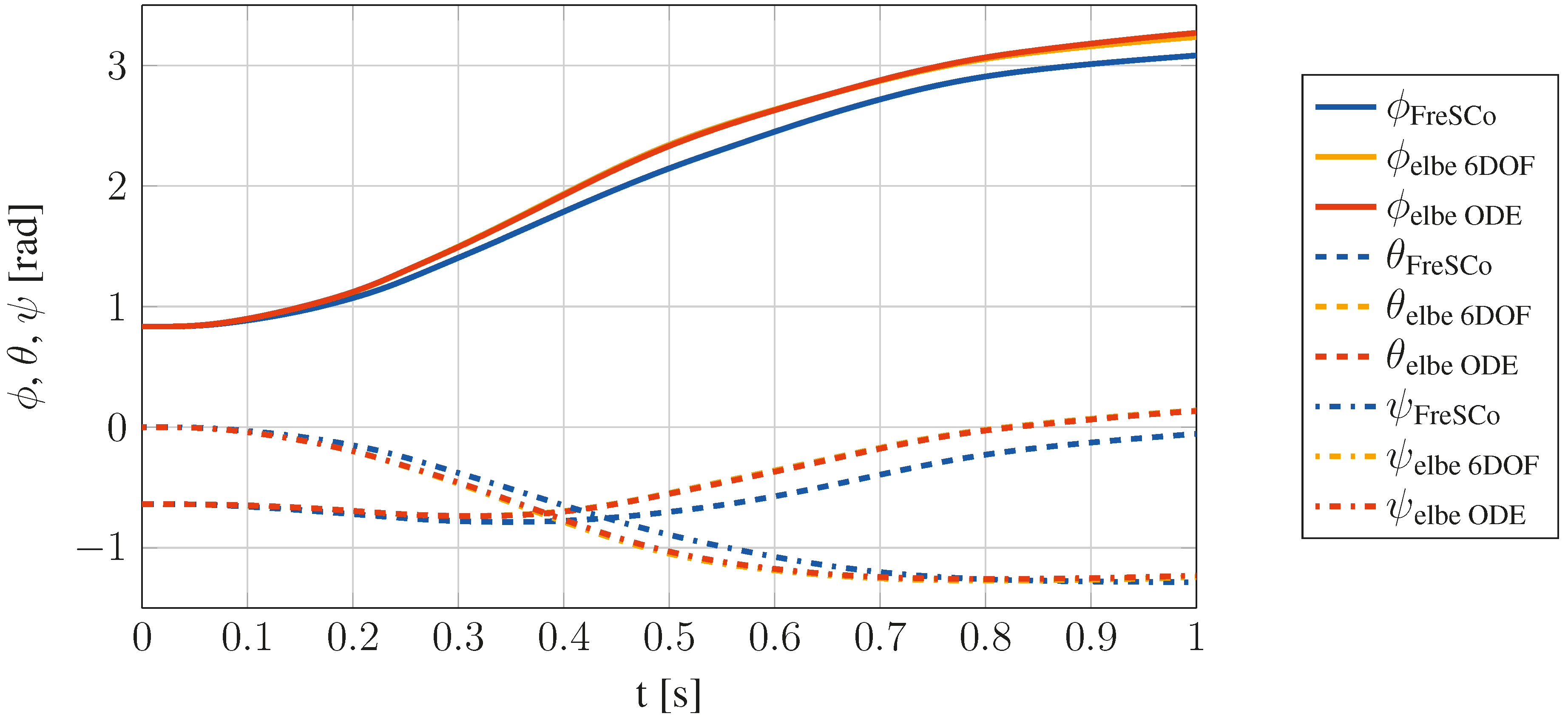
4.1. Validation of the Coupling Methodology


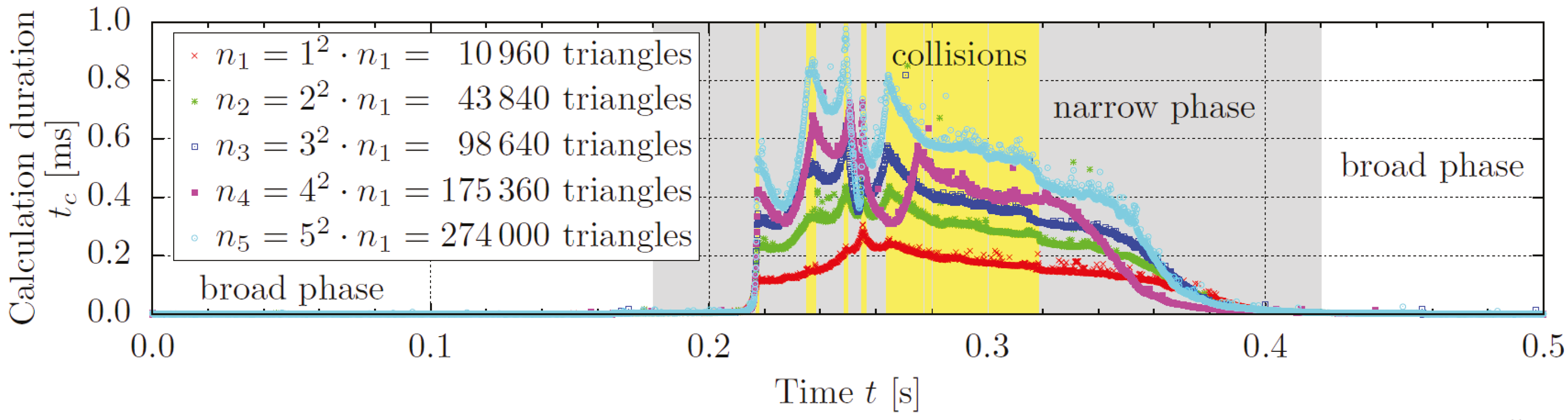
4.2. ODE Performance Considerations
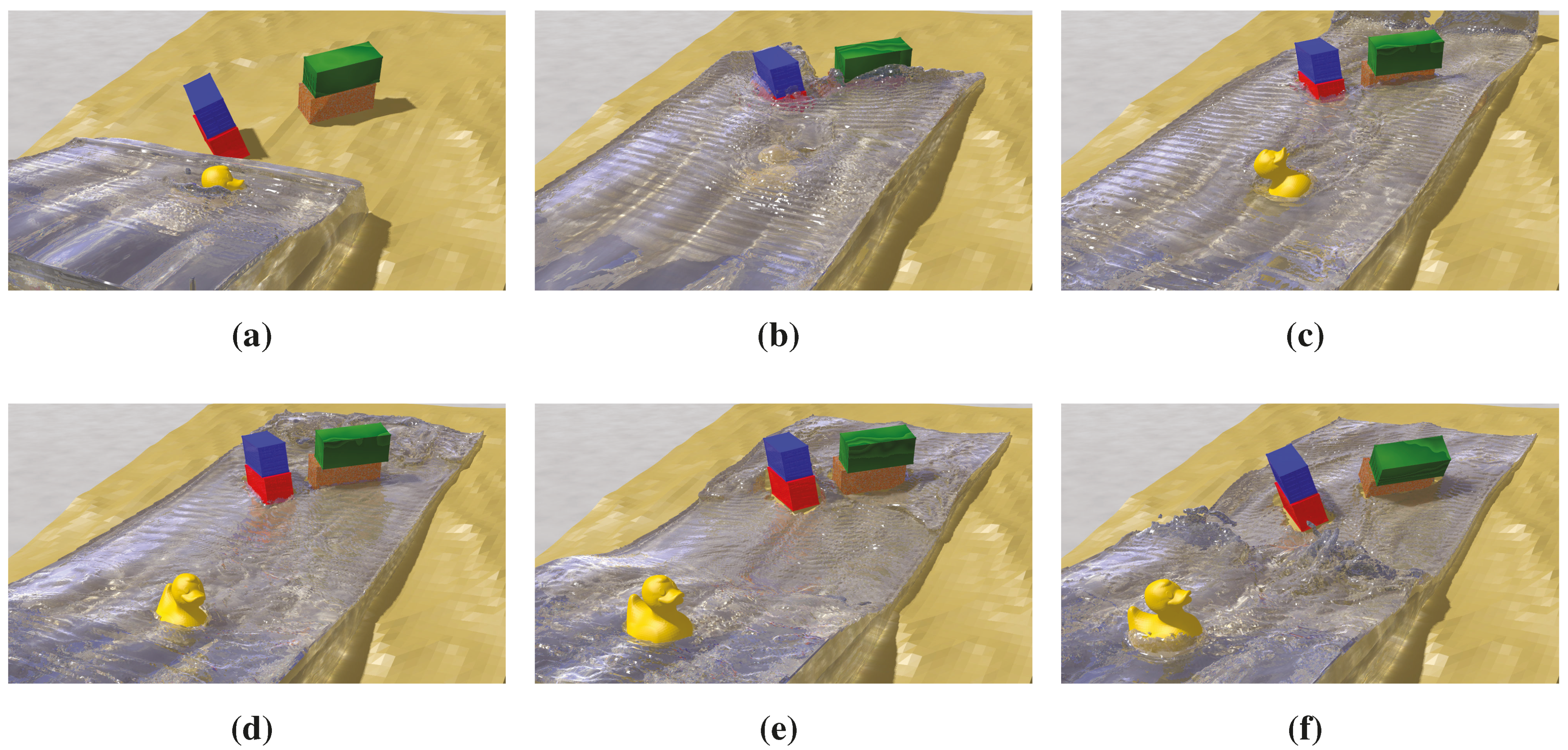
4.3. Debris Flow Application
| Domain | 2.0 m × 0.8 m × 0.5 m (1:10) | Restitution coefficient | 0.5 |
| Lattice | 400 × 160 × 100 | Friction coefficient | 0.5 |
| Δx | 0.005 m | ||
| Δt | 3E−5 s | Number of triangles | |
| Re | 750,000 | Bathymetry | 8958 |
| Fr | 5.3 | Containers | 4 × 1730 |
| Ma | 0.05 | Duck | 10,960 |
5. Dam Break Simulations
5.1. Bund Wall Overtopping
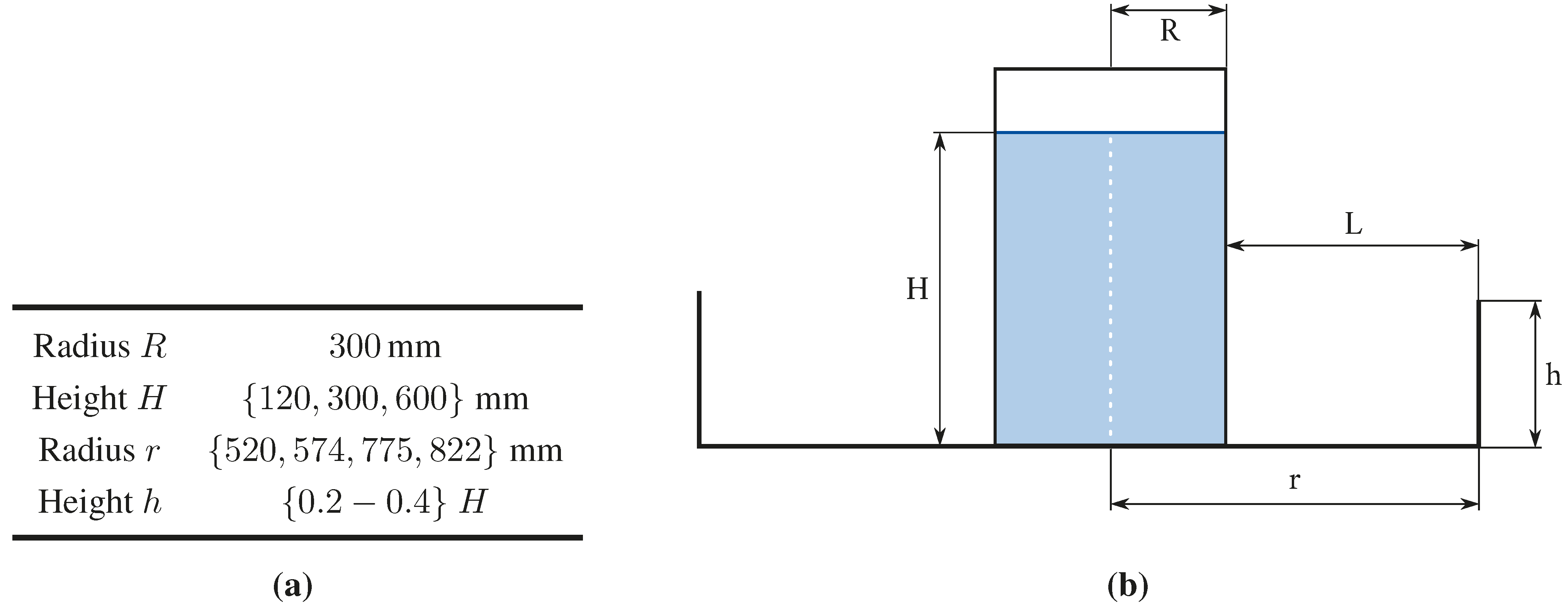
| Case | Tank | Bund | Case | Q (%) | p (-) | εQ | εp | ||||||
|---|---|---|---|---|---|---|---|---|---|---|---|---|---|
| R (mm) | H (mm) | r (mm) | h (mm) | exp. | num. | exp. | num. | ||||||
| 1 | 300 | 120 | 574 | 36 | 1 | 32.00 | 30.99 | 1.32 | 1.27 | 0.03 | 0.04 | ||
| 2 | 300 | 300 | 574 | 90 | 2 | 38.00 | 36.87 | 1.97 | 1.93 | 0.03 | 0.02 | ||
| 3 | 300 | 600 | 574 | 180 | 3 | 34.00 | 28.95 | 1.79 | 1.97 | 0.15 | −0.10 | ||
| 4 | 300 | 120 | 520 | 48 | 4 | 22.00 | 24.88 | 2.01 | 2.13 | −0.13 | −0.06 | ||
| 5 | 300 | 300 | 520 | 120 | 5 | 26.00 | 29.90 | 1.65 | 1.88 | −0.15 | −0.14 | ||
| 6 | 300 | 600 | 520 | 240 | 6 | 21.00 | 24.37 | 1.82 | 1.74 | −0.16 | 0.04 | ||
| 7 | 300 | 120 | 822 | 24 | 7 | 28.00 | 30.65 | 4.12 | 3.49 | −0.09 | 0.15 | ||
| 8 | 300 | 300 | 822 | 60 | 8 | 45.00 | 38.26 | 2.80 | 3.00 | 0.15 | −0.07 | ||
| 9 | 300 | 600 | 822 | 120 | 9 | 43.00 | 36.87 | 2.22 | 2.24 | 0.14 | −0.01 | ||
| 10 | 300 | 120 | 775 | 36 | 10 | 15.00 | 16.68 | 2.09 | 1.87 | −0.11 | 0.11 | ||
| 11 | 300 | 300 | 775 | 90 | 11 | 24.00 | 25.22 | 1.35 | 1.59 | −0.05 | −0.17 | ||
| 12 | 300 | 600 | 775 | 180 | 12 | 24.00 | 27.10 | 1.23 | 1.24 | −0.13 | −0.01 | ||

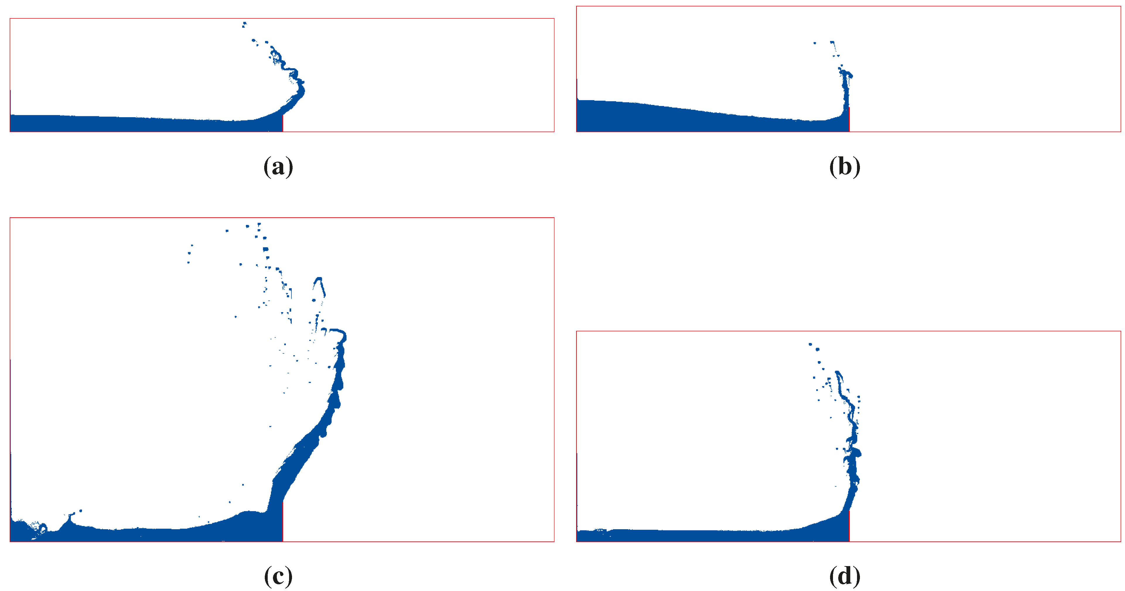
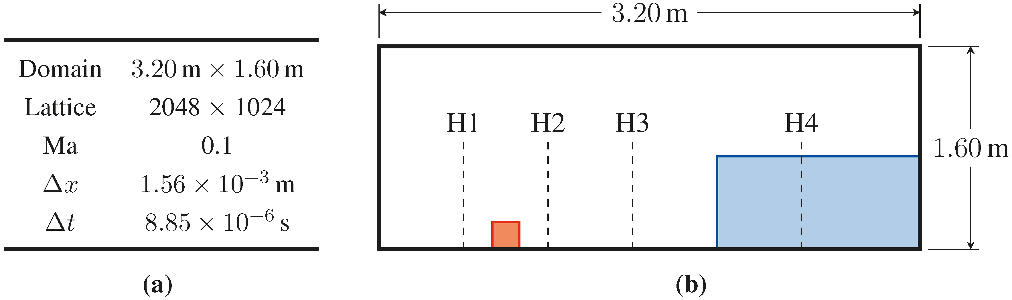
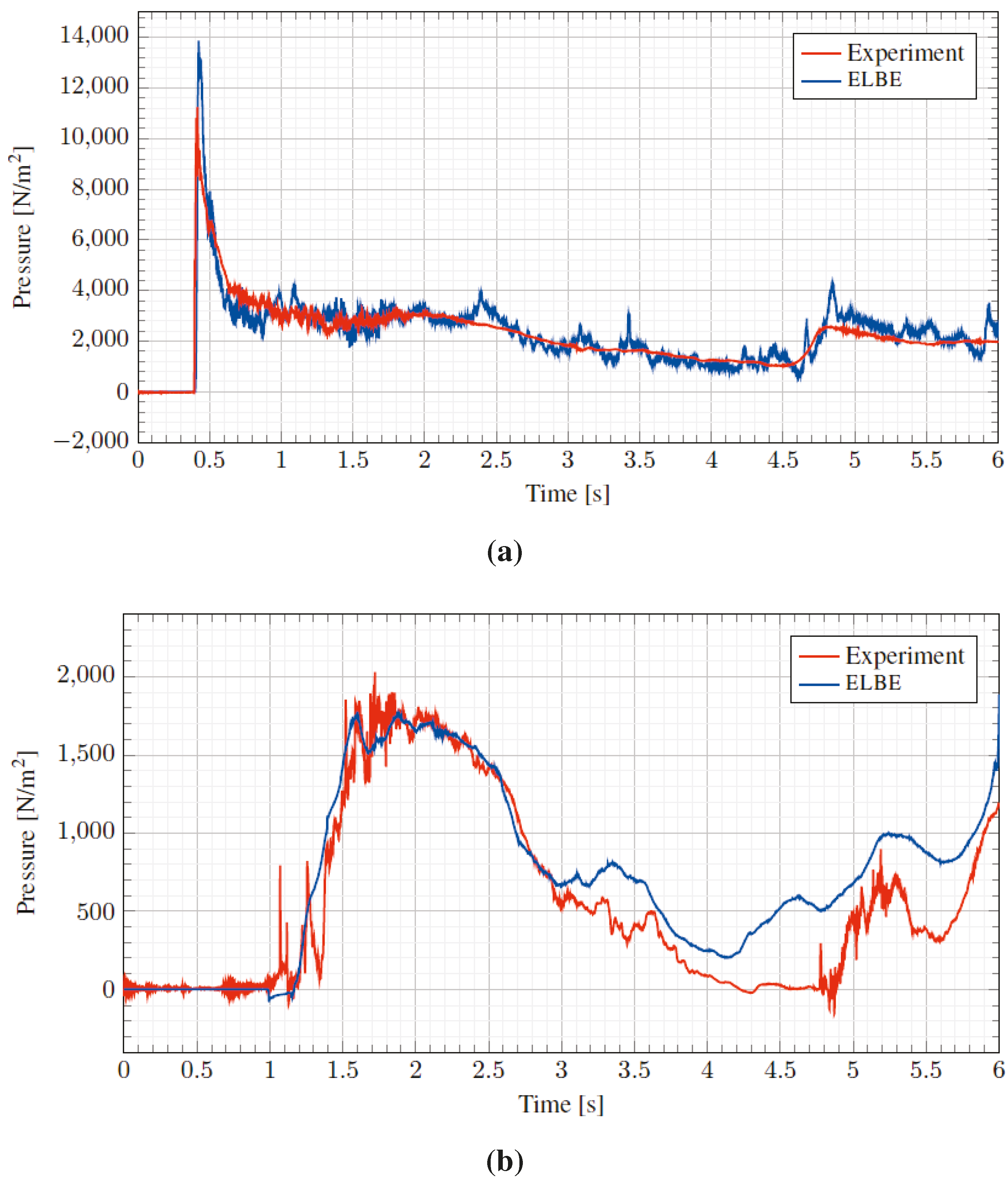
5.2. Wave Impact


6. Numerical Wave Tank for On- and Off-Shore Structures
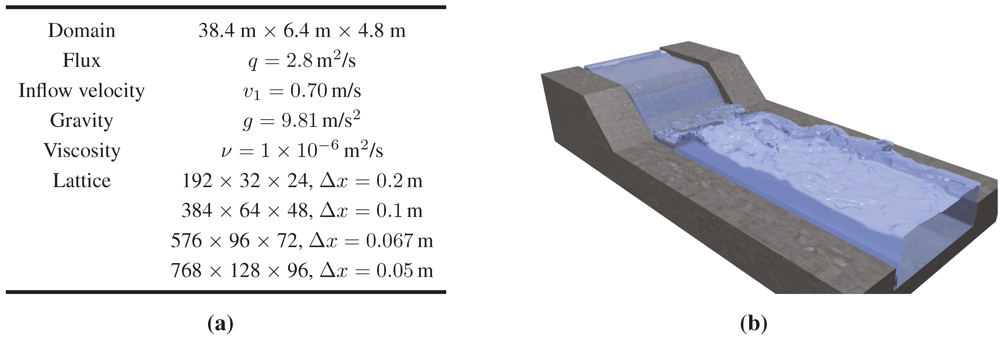
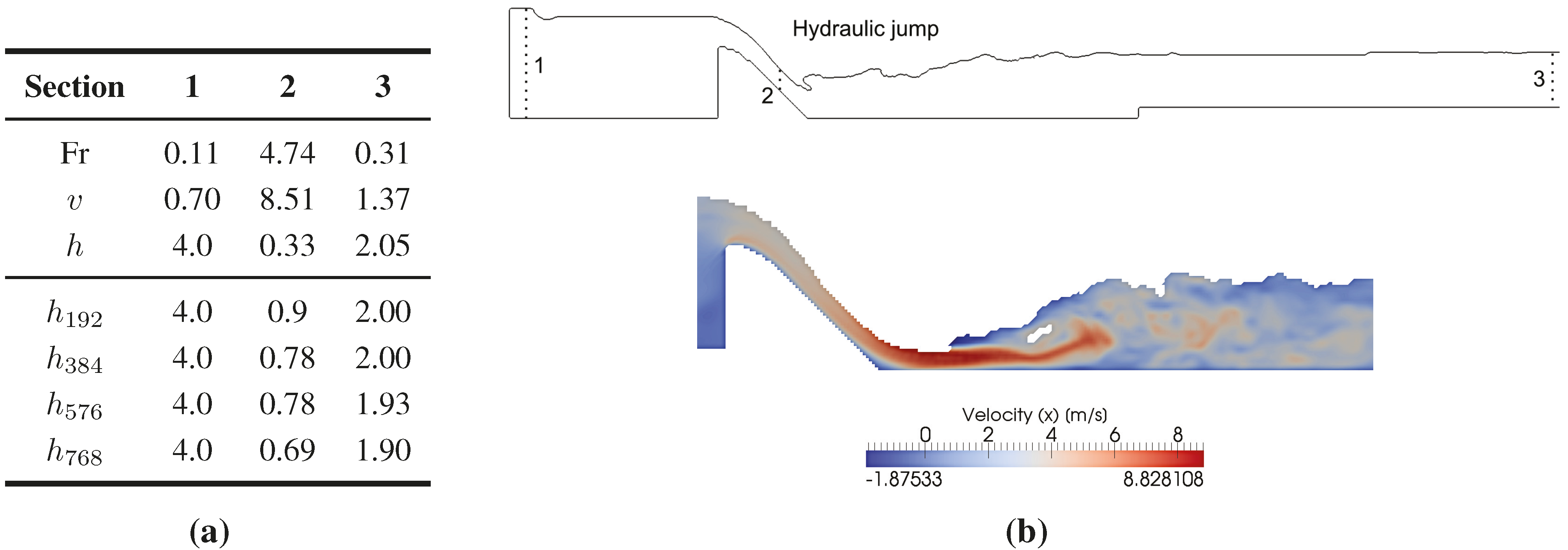
6.1. River Engineering

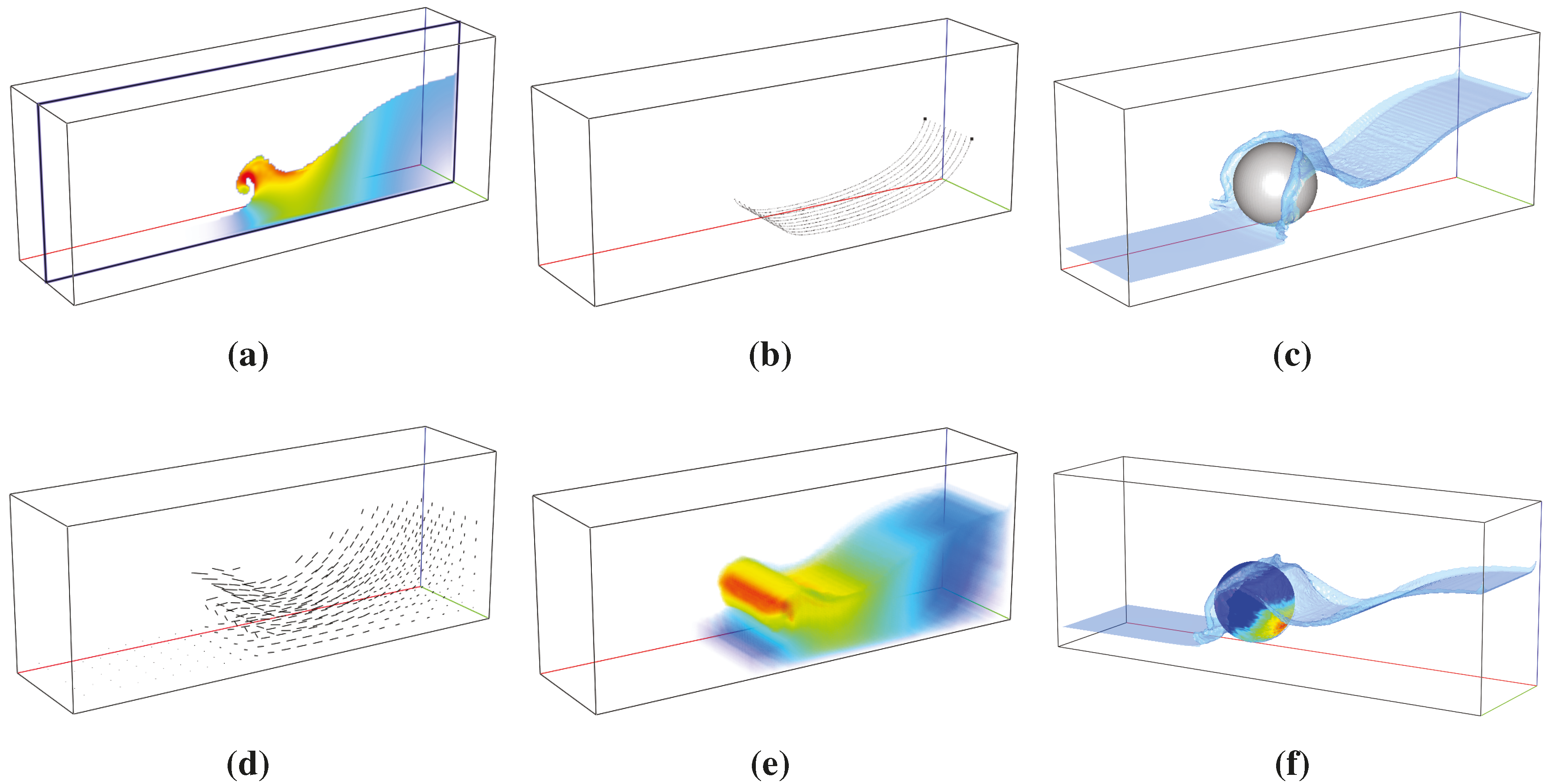
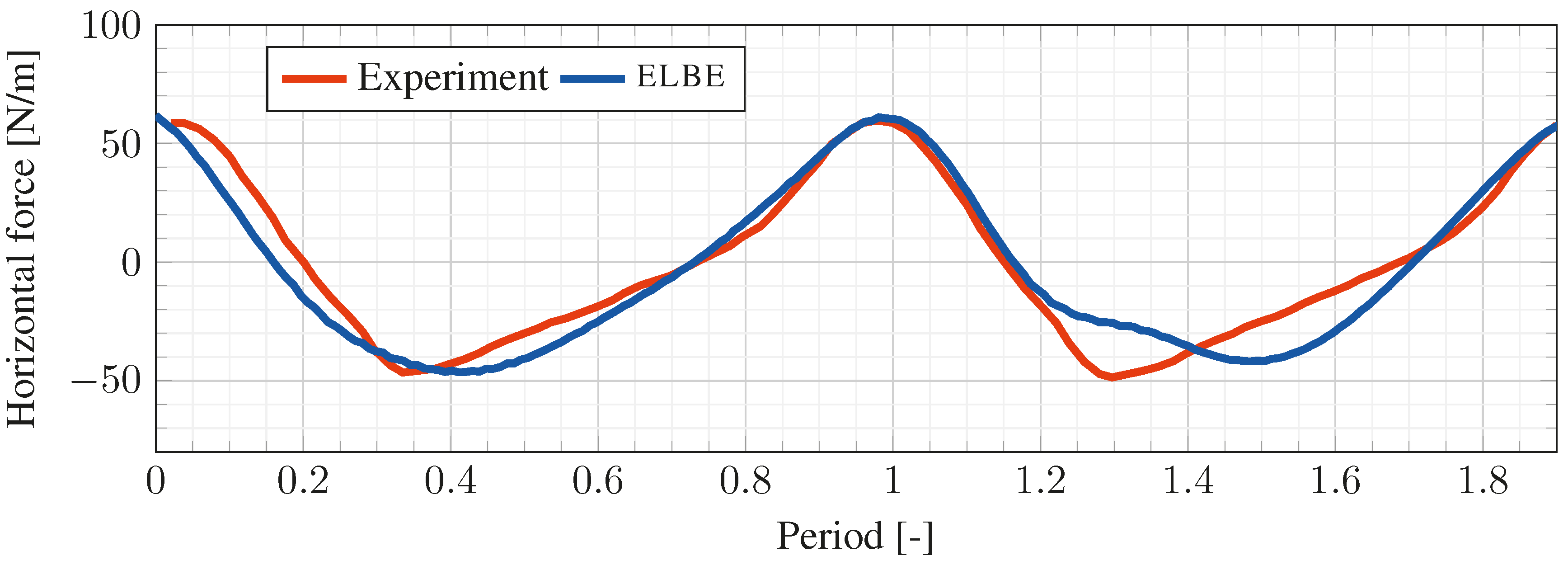
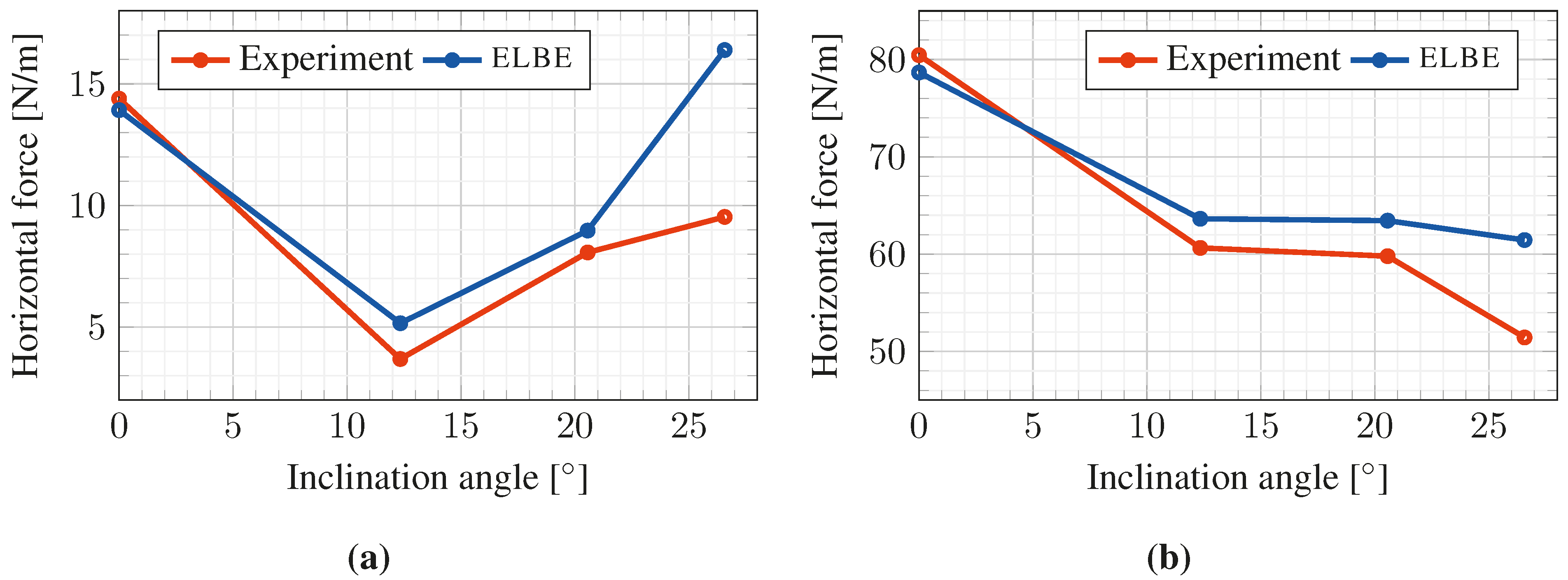
6.2. Wave-Current-Induced Loads on Submerged Bodies
| Geometry | Current C3 | Waves H3 | |||
|---|---|---|---|---|---|
| # | Exp. | elbe | Exp. | elbe | |
| 1 | 14.39 | 13.92 | 80.45 | 78.67 | |
| 2 | 3.69 | 5.16 | 60.64 | 63.64 | |
| 3 | 8.07 | 8.97 | 59.79 | 63.44 | |
| 5 | 9.53 | 16.39 | 51.44 | 61.45 | |

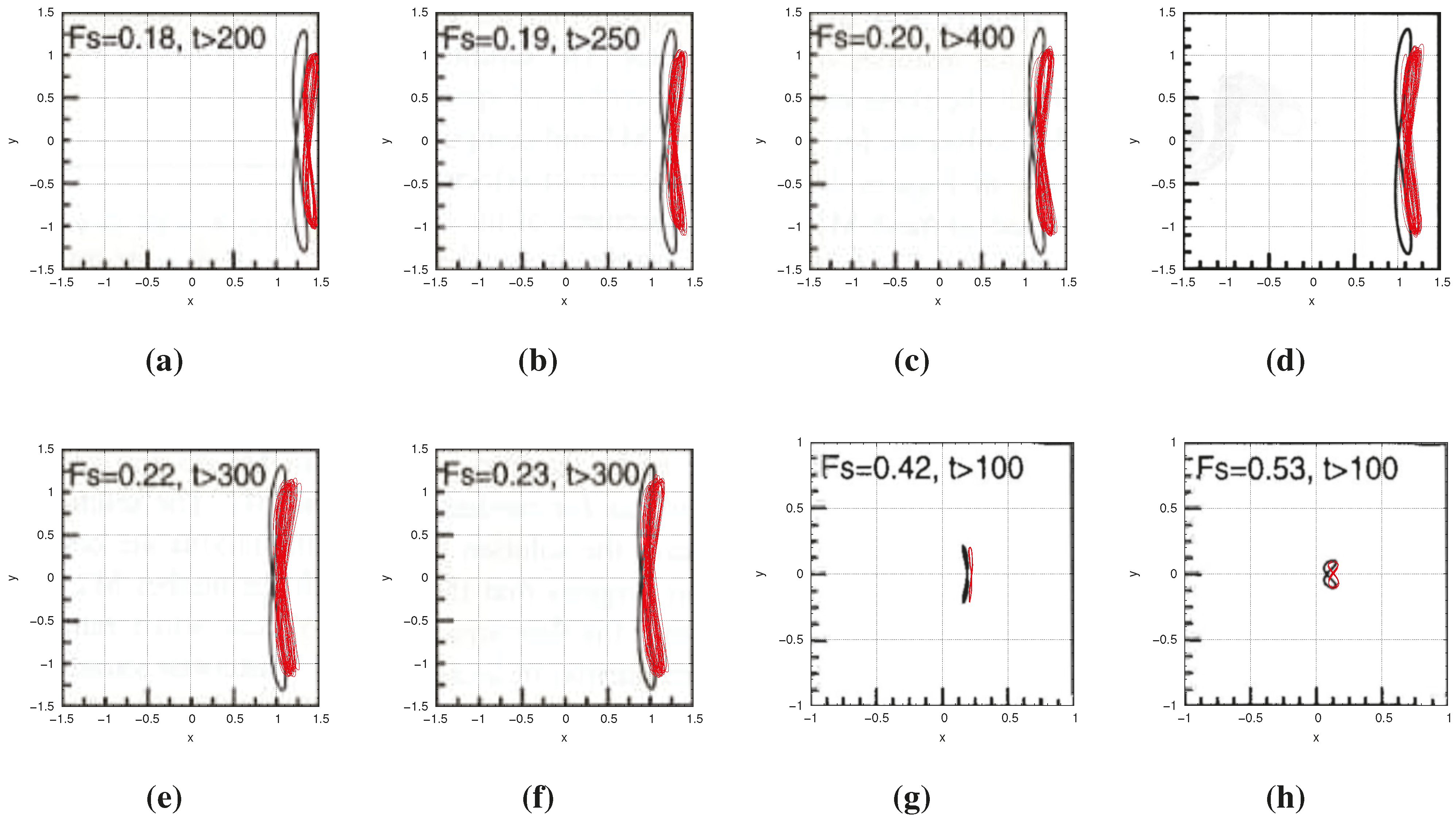
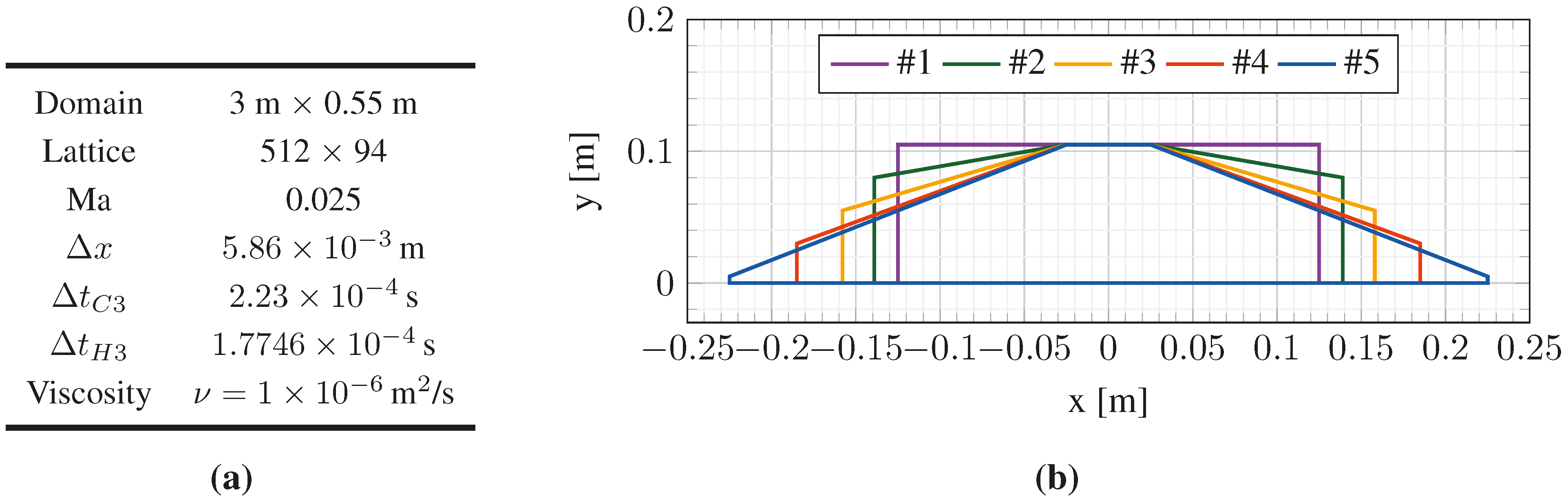
6.3. Vortex-Induced Vibrations
| Domain | 3.20 m × 1.60 m |
| Lattice | 512 × 256 |
| Δx | 0.47 m, 0.23 m |
| Reynolds number Re | 325 |
| Strouhal number Fs | 0.18–0.53 |
| Dimensionless mass | 4.7273 |
| Lehr’s damping ratio | 0.00033 |

7. Summary and Conclusions
Acknowledgments
Author Contributions
Conflicts of Interest
References
- Le Touzé, D.; Grenier, N.; Barcarolo, D.A. 2nd International Conference on Violent Flows. Available online: http://www.publibook.com/librairie/livre.php?isbn=9782748390353 (accessed on 7 July 2015).
- Dean, R.G.; Dalrymple, R.A. Water Wave Mechanics for Engineers and Scientists; World Scientific Publishing: Singapore, 1991. [Google Scholar]
- Dunbar, P.; McCullough, H.; Mungov, G.; Varner, J.; Stroker, K. 2011 Tohoku earthquake and tsunami data available from the National Oceanic and Atmospheric Administration/National Geophysical Data Center. Geomat. Nat. Hazards Risk 2011, 2, 305–323. [Google Scholar] [CrossRef]
- Synolakis, C.; Bernard, E. Tsunami science before and beyond Boxing Day 2004. Philos. Trans. A Math. Phys. Eng. Sci. 2006, 364, 2231–2265. [Google Scholar] [CrossRef] [PubMed]
- Wienke, J.; Oumeraci, H. Breaking wave impact force on a vertical and inclined slender pile—Theoretical and large-scale model investigations. Coast. Eng. 2005, 52, 435–462. [Google Scholar] [CrossRef]
- D’Humieres, D.; Ginzburg, I.; Krafczyk, M.; Lallemand, P.; Luo, L.S. Multiple-Relaxation-Time Lattice Boltzmann models in three dimensions. R. Soc. Lond. Philos. Trans. Ser. A 2002, 360, 437–451. [Google Scholar] [CrossRef] [PubMed]
- Ginzburg, I.; Steiner, K. Lattice Boltzmann model for free-surface flow and its application to filling process in casting. J. Comput. Phys. 2003, 185, 61–99. [Google Scholar] [CrossRef]
- Junk, M.; Yang, Z. Pressure boundary condition for the lattice Boltzmann method. Comput. Math. Appl. 2009, 58, 922–929. [Google Scholar] [CrossRef]
- Krafczyk, M.; Tölke, J.; Luo, L.S. Large-eddy simulations with a multiple-relaxation-time LBE model. Int. J. Mod. Phys. B 2003, 17, 33–39. [Google Scholar] [CrossRef]
- He, X.; Luo, L.S. Lattice Boltzmann model for the incompressible Navier-Stokes equation. J. Stat. Phys. 1997, 88, 927–944. [Google Scholar] [CrossRef]
- Körner, C.; Thies, M.; Hofmann, T.; Thürey, N.; Rüde, U. Lattice Boltzmann Model for Free Surface Flow for Modeling Foaming. J. Stat. Phys. 2005, 121, 179–196. [Google Scholar] [CrossRef]
- Guo, Z.; Zheng, C.; Shi, B. Discrete lattice effects on the forcing term in the lattice Boltzmann method. Phys. Rev. E 2002, 65, 046308. [Google Scholar] [CrossRef]
- Janßen, C.; Krafczyk, M. A lattice Boltzmann approach for free-surface-flow simulations on non-uniform block-structured grids. Comput. Math. Appl. 2010, 59, 2215–2235. [Google Scholar] [CrossRef]
- Donath, S.; Feichtinger, C.; Pohl, T.; Götz, J.; Rüde, U. A Parallel Free Surface Lattice Boltzmann Method for Large-Scale Applications. In Parallel Computational Fluid Dynamics: Recent Advances and Future Directions; DEStech Publications: Lancaster, PA, USA, 2010; pp. 318–330. [Google Scholar]
- Anderl, D.; Bogner, S.; Rauh, C.; Rüde, U.; Delgado, A. Free surface lattice Boltzmann with enhanced bubble model. Comput. Math. Appl. 2014, 67, 331–339. [Google Scholar] [CrossRef]
- Janßen, C.; Krafczyk, M. Free surface flow simulations on GPGPUs using LBM. Comput. Math. Appl. 2011, 61, 3549–3563. [Google Scholar] [CrossRef]
- Geller, S. Ein explizites Modell für die Fluid-Struktur-Interaktion basierend auf LBM und p-FEM. Ph.D. Thesis, TU Carolo-Wilhelmina zu Braunschweig, Braunschweig, Germany, 2010. [Google Scholar]
- Geller, S.; Kollmannsberger, S.; Bettah, M.; Scholz, D.; Düster, A.; Krafczyk, M.; Rank, E. An explicit model for three dimensional fluid structure-interaction using LBM and p-FEM. In Fluid-Structure Interaction II; Bungartz, H.J., Schäfer, M., Eds.; Lecture Notes in Computational Science and Engineering; Springer: Berlin/Heidelberg, Germany, 2010; pp. 285–325. [Google Scholar]
- Janßen, C.F.; Koliha, N.; Rung, T. A fast and rigorously parallel surface voxelization technique for GPGPU-accelerated CFD simulations. Commun. Comput. Phys. 2015. [Google Scholar] [CrossRef]
- Stewart, D.E.; Trinkle, J.C. An Implicit Time-Stepping Scheme for Rigid Body Dynamics with Inelastic Collisions and Coulomb Friction. Int. J. Numer. Methods Eng. 1996, 39, 2673–2691. [Google Scholar] [CrossRef]
- Boeing, A.; Bräunl, T. Evaluation of Real-Time Physics Simulation Systems. In Proceedings of the 5th International Conference on Computer Graphics and Interactive Techniques in Australia and Southeast Asia, Perth, Australia, 1–4 December 2007; pp. 281–288.
- Hummel, J.; Wolff, R.; Stein, T.; Gerndt, A.; Kuhlen, T. An Evaluation of Open Source Physics Engines for Use in Virtual Reality Assembly Simulations. Adv. Vis. Comput. 2012, 7432, 346–357. [Google Scholar]
- Metrikin, I.; Borzov, A.; Lubbad, R.; Løset, S. Numerical Simulation of a Floater in a Broken-Ice Field: Part II—Comparative Study of Physics Engines. In Proceedings of the 31st International Conference on Ocean, Offshore and Arctic Engineering (OMAE2012), Rio de Janeiro, Brazil, 1–6 July 2012; Volume 6, pp. 477–486.
- Tölke, J.; Krafczyk, M. Implementation of a Lattice Boltzmann kernel using the Compute Unified Device Architecture developed by nVIDIA. Comput. Vis. Sci. 2008, 1, 29–39. [Google Scholar] [CrossRef]
- Tölke, J.; Krafczyk, M. TeraFLOP computing on a desktop PC with GPUs for 3D CFD. Int. J. Comput. Fluid Dyn. 2008, 22, 443–456. [Google Scholar] [CrossRef]
- NVIDIA. List of GPU-Accelerated Applications. 2015. Available online: http://www.nvidia.com/object/gpu-applications.html (accessed on 15 January 2015).
- Grilli, S.; Harris, J.; Tajalibakhsh, T.; Kirby, J.; Shi, F.; Masterlark, T.; Kyriakopoulos, C. Numerical simulation of the 2011 Tohoku tsunami: Comparison with field observations and sensitivity to model parameter. In Proceedings of the 22nd Offshore and Polar Engineering Conference, ISOPE12, Rodos, Greece, 17–23 June 2012.
- Ocean Networks Canada. A Tsunami Detection Initiative for British Columbia; Workshop Report; Port Alberni (Canada), 27–28 March 2014; Ocean Networks Canada, University of Victoria: Victoria, BC, Canada, 2014. [Google Scholar]
- Kowalik, Z.; Murty, T.S. Numerical Modeling of Ocean Dynamics; World Scientific Publishing: Singapore, 1993. [Google Scholar]
- Wei, G.; Kirby, J.; Grilli, S.; Subramanya, R. A fully nonlinear Boussinesq model for surface waves. I. Highly nonlinear, unsteady waves. J. Fluid Mech. 1995, 294, 71–92. [Google Scholar]
- Shi, F.; Kirby, J.; Harris, J.; Geiman, J.; Grilli, S. A high-order adaptive time-stepping TVD solver for Boussinesq modeling of breaking waves and coastal inundation. Ocean Model. 2012, 43–44, 36–51. [Google Scholar] [CrossRef]
- Zhou, J. Lattice Boltzmann Methods for Shallow Water Flows; Springer: Berlin/Heidelberg, Germany, 2003. [Google Scholar]
- Chopard, B.; Pham, V.; Lefevre, L. Asymmetric lattice Boltzmann model for shallow water flows. Comput. Fluids 2013, 88, 225–231. [Google Scholar] [CrossRef]
- Frandsen, J. Investigations of wave runup using a LBGK modeling approach. In Proceedings of the XVI International Conference on Computational Methods in Water Resoures, Copenhagen, Denmark, 18–22 June 2006.
- Thömmes, G.; Seaid, M.; Banda, M.K. Lattice Boltzmann methods for shallow water flow applications. Int. J. Numer. Meth. Fluids 2007, 55, 673–692. [Google Scholar] [CrossRef]
- Tubbs, K. Lattice Boltzmann Modeling for Shallow Water Equations Using High Performance Computing. Ph.D. Thesis, Lousiana State University, Baton Rouge, LA, USA, May 2010. [Google Scholar]
- Janßen, C.; Bengel, S.; Rung, T.; Dankowski, H. A fast numerical method for internal flood water dynamics to simulate water on deck and flooding scenarios of ships. In Proceedings of the 32nd International Conference on Ocean, Offshore and Arctic Engineeing (OMAE), Nantes, France, 9–14 June 2013.
- Liu, P.F.; Yeh, H.; Synolakis, C. Advanced Numerical Models for Simulating Tsunami Waves and Runup; World Scientific Publishing: Singapore, 2008. [Google Scholar]
- Catalina 2004: The third international workshop on long-wave runup models. Benchmark problems #1 – #4. Available online: http://isec.nacse.org/workshop/2004_cornell/benchmark.html (accessed on 15 January 2015).
- Carrier, G.F.; Wu, T.T.; Yeh, H. Tsunami run-up and draw-down on a plane beach. J. Fluid Mech. 2003, 475, 79–99. [Google Scholar] [CrossRef]
- Frandsen, J. A simple LBE wave runup model. Prog. Comput. Fluid Dyn. 2008, 8, 222–232. [Google Scholar] [CrossRef]
- Shi, F.; Kirby, J.T.; Tehranirad, B.; Harris, J.C. FUNWAVE-TVD, Documentation and Users’ Manual; Research Report, cacr-11-04; University of Delaware: Newark, DE, USA, 2011. [Google Scholar]
- Amante, C.; Eakins, B.W. ETOPO1 1 Arc-Minute Global Relief Model: Procedures, Data Sources and Analysis. NOAA Technical Memorandum NESDIS NGDC-24. Available online: https://www.ngdc.noaa.gov/mgg/global/relief/ETOPO1/docs/ETOPO1.pdf (accessed on 7 July 2015).
- Okada, Y. Surface deformation due to shear and tensile faults in a half-space. Bull. Seismol. Soc. Am. 1985, 75, 1135–1154. [Google Scholar]
- Kraskowski, M. Validation of the RANSE Rigid Body Motion Computations. In Proceedings of the 12th Numerical Towing Tank Symposium, Cortona, Italy, 4–6 October 2009; Volume 6, pp. 99–104.
- Willie. Rubber Duck. 2013. Available online: http://www.thingiverse.com/thing:139894 (accessed on 15 January 2015).
- Martin, J.C.; Moyce, W.J. Part IV. An Experimental Study of the Collapse of Liquid Columns on a Rigid Horizontal Plane. Philos. Trans. R. Soc. Lond. A 1952, 244, 312–324. [Google Scholar] [CrossRef]
- Atherton, W.; Ash, J.W.; Alkhaddar, R.M. An Experimental Investigation of Bund Wall Overtopping and Dynamic Pressures on the Bund Wall Following Catasrophic Failure of a Storage Vessel; Research Report 333; Liverpool John Moores University: Liverpool, UK, 2005. [Google Scholar]
- Kleefsman, K.M.T. Water Impact Loading on Offshore Structures—A Numerical Study. Ph.D. Thesis, University of Groningen, Groningen, The Netherlands, 18 November 2005. [Google Scholar]
- Wemmenhove, R. Numerical Simulation of Two-Phase Flow in Offshore Environments. Ph.D. Thesis, Rijksuniversiteit Groningen, Groningen, The Netherlands, 16 May 2008. [Google Scholar]
- Chow, V.T. Open-Channel Hydraulics; MC Graw-Hill: New York, NY, USA, 1959. [Google Scholar]
- Markus, D.; Ferri, F.; Wüchner, R.; Frigaard, P.; Bletzinger, K.-U. Complementary numerical-experimental benchmarking for shape optimization and validation of structures subjected to wave and current forces. Comput. Fluids 2014, 118, 69–88. [Google Scholar] [CrossRef]
- Mittal, S.; Kumar, V. Finite element study of vortex-induced cross-flow and in-line oscillations of a circular cylinder at low Reynolds numbers. Int. J. Numer. Methods Fluids 1999, 31, 1087–1120. [Google Scholar] [CrossRef]
- Janßen, C.F.; Koliha, N.; Rung, T. Online visualization and interactive monitoring of real-time simulations of complex turbulent flows on off-the-shelf commodity hardware. Comput. Vis. Sci. 2015. submitted. [Google Scholar]
© 2015 by the authors; licensee MDPI, Basel, Switzerland. This article is an open access article distributed under the terms and conditions of the Creative Commons Attribution license (http://creativecommons.org/licenses/by/4.0/).
Share and Cite
Janßen, C.F.; Mierke, D.; Überrück, M.; Gralher, S.; Rung, T. Validation of the GPU-Accelerated CFD Solver ELBE for Free Surface Flow Problems in Civil and Environmental Engineering. Computation 2015, 3, 354-385. https://doi.org/10.3390/computation3030354
Janßen CF, Mierke D, Überrück M, Gralher S, Rung T. Validation of the GPU-Accelerated CFD Solver ELBE for Free Surface Flow Problems in Civil and Environmental Engineering. Computation. 2015; 3(3):354-385. https://doi.org/10.3390/computation3030354
Chicago/Turabian StyleJanßen, Christian F., Dennis Mierke, Micha Überrück, Silke Gralher, and Thomas Rung. 2015. "Validation of the GPU-Accelerated CFD Solver ELBE for Free Surface Flow Problems in Civil and Environmental Engineering" Computation 3, no. 3: 354-385. https://doi.org/10.3390/computation3030354
APA StyleJanßen, C. F., Mierke, D., Überrück, M., Gralher, S., & Rung, T. (2015). Validation of the GPU-Accelerated CFD Solver ELBE for Free Surface Flow Problems in Civil and Environmental Engineering. Computation, 3(3), 354-385. https://doi.org/10.3390/computation3030354