Computational Triangulation in Mathematics Teacher Education

Abstract

The paper is written to demonstrate the applicability of the notion of triangulation typically used in social sciences research to computationally enhance the mathematics education of future K-12 teachers. The paper starts with the so-called Brain Teaser used as background for (what is called in the paper) computational triangulation in the context of four digital tools. Computational problem solving and problem formulating are presented as two sides of the same coin. By revealing the hidden mathematics of Fibonacci numbers included in the Brain Teaser, the paper discusses the role of computational thinking in the use of the well-ordering principle, the generating function method, digital fabrication, difference equations, and continued fractions in the development of computational algorithms. These algorithms eventually lead to a generalized Golden Ratio in the form of a string of numbers independently generated by digital tools used in the paper.

1. Introduction

In the mid 20th century, the concept of triangulation was introduced in social sciences research to make the domain more rigorous [1,2,3]. Mathematics education, as the modern-day field of disciplined inquiry [4], uses triangulation as an inquiry tool of social sciences towards overcoming the limitations of the interview-based qualitative research methods [5], debating the correctness of proof from a philosophical perspective [6], and using multiple solution strategies in problem solving [7]. In the age of technology, with the ubiquity of computational thinking [8] in diverse disciplines, the methodology of triangulation became integrated with advances in digital technology, allowing for scientific experiments to be validated by more than one computational instrument thus enhancing the credibility of problem solving [9].

Computational triangulation is a new (two-word) term apparently not used in the literature, either mathematical or educational. The paper is written to introduce this term in the specific context of mathematics teacher education. Conceptually, the term grew out of the author’s experience of using computers with future K-12 teachers of mathematics and interest in social sciences research which had been enriched by the triangulation approach to sociology [1,2,3]. Linguistically, the term was formed when the author was invited to contribute a paper to the special issue “Computational social science and complex systems” of Computation. The use of sophisticated software tools in education, which nowadays is increasingly supported by various learning management systems, enables prospective teachers to appreciate the intrinsic complexity of the systems as agency that erases geographical boundaries of interpersonal collaboration in the rigorous study of school mathematics. Through the lens of this agency, the computational triangulation of solutions to certain problems used in mathematics teacher education may be seen as a replacement of “the traditional social process of proof” [10] (p. 1402) to avoid both subtle and unsubtle errors in problem solving in the digital era.

The paper provides mathematics education examples of using digital tools in support of computational triangulation as the social sciences construct including the triangulation within and between methods [11] and the control of internal and external rival factors [12]. Triangulation within and between methods in problem solving are interpreted, respectively, in terms of the comparison of multiple techniques within a single method and proving the equivalence of symbolic computations provided by different digital instruments. Internal and external rival factors and their control in problem solving and posing are interpreted, respectively, as balancing the diversity of skills in using computational tools to support mathematical visualization and navigating through the wealth of technology and problem-solving methods available.

The paper’s structure is as follows. First, materials (software, publications, and teaching standards) and methods (specific for mathematics education) used by the author are described. Mathematical content begins with a problem about cookies on plates and four different computational solutions are discussed. Then, the presence of Fibonacci-like numbers in the problem is revealed, leading to the conceptual generalization needed for more effective computations interpreted through the lens of a triangulation approach to sociology. Finally, the paper discusses the importance of having a more knowledgeable other in the classroom in order to recognize an accidental discovery by a student of a new mathematical phenomenon which is then further explored under the umbrella of a multi-instrument computational triangulation. It concludes by emphasizing the role of concrete problems and digital tools in the teaching of the intrinsically abstract subject matter of mathematics.

2. Materials and Methods

Three types of materials have been used by the author when working on this paper. The first type is digital, the so-called “mathematical action technologies” [13] (p. xi). These technologies include computational knowledge engine Wolfram Alpha developed by Wolfram Research [www.woframalpha.com, accessed on 7 February 2023] and the mathematical software Maple [14] used by the author for symbolic computations, an electronic spreadsheet characterized as “an electronic blackboard and electronic chalk in a classroom” [15] and used by the author as a tool for numeric modeling, and computer algebra system Graphing Calculator produced by Pacific Tech [16] that supported computational triangulation activities with mathematical visualization.

The second type of materials included literature on triangulation as a concept used by sociologists to cement inquiry with rigor thus making it truly disciplined [1,2,3,5,11,12,17,18]. As was mentioned in the introduction, the need for rigor was one of the main reasons for introducing the concept of triangulation into sociology. At the same time, rigor is necessary for the success of ideas in the age of technology. Whereas technological innovations might make curious minds completely dependent on digital tools, the tools are still created by humans who, unfortunately, are susceptible to errors. Thus, the notion of computational triangulation should not be neglected.

The third type of materials used by the author included teaching and learning mathematics standards used across six continents by countries such as Australia [19], Canada [20,21], Chile [22], England [23], Singapore [24], South Africa [25], and the United States [26,27,28]. The standards uniformly call for fostering mathematical reasoning in the technological paradigm and using computer-generated representations of concepts when solving and posing problems. As will be shown in the paper, computational triangulation encourages and supports these mathematics education activities.

Methods specific for mathematics education used in this paper include computer-based mathematics education, standards-based mathematics, problem solving and problem posing. In particular, those methods are conducive to presenting “teacher candidates with experiences in mathematics relevant to their chosen profession” [28] (p. 137). In the United States, many secondary mathematics teacher preparation programs offer courses “that include topics such as … finite difference equations, iteration and recursion … and computer programming” [27] (p. 66). These topics underpin algorithms of computational triangulation used in this paper. The university where the author has been preparing teacher candidates to teach mathematics is located in upstate New York in close proximity to Canada, and many of the author’s students are Canadians pursuing their master’s degrees in education. As future teachers of mathematics, they learn how to think computationally by “expressing problems in such a way that their solutions can be reached using computational steps and algorithms” [20] (p. 513). This diversity of students suggests the importance of aligning mathematics education courses with multiple international perspectives on teaching and learning mathematics in the digital era.

3. Triangulation within a Method

The following problem, in a slightly different formulation, was offered to a class of elementary teacher candidates, the author’s students, enrolled in a mathematics content course within a graduate program in childhood instruction. The problem was a prelude to celebrated Fibonacci numbers (not directly mentioned in the problem) that the candidates were soon to study including the recursive and closed (Binet’s) formulas. Binet’s formula was introduced in the course as an illustration of one of the profound ideas of mathematics—integers can be represented through other types of numbers; in particular, Fibonacci numbers can be represented through an exponential arrangement of the Golden Ratio and its reciprocal. In the true spirit of computational triangulation, Binet’s formula as a generator of Fibonacci numbers was verified by the candidates using a spreadsheet and Wolfram Alpha (free version). In this paper, the presence of Fibonacci numbers in the problem offered to the candidates will be revealed as means of developing computational environments necessary for applying triangulation to mathematical problem solving. To begin, consider:

• Brain Teaser: Five identical plates are lined up and each one is filled with candies. How many ways can one put candies on the first two plates so that when each plate beginning from the third has as many candies as the previous two plates combined, the fifth plate has 13 candies?
• Discussion: As a method of solving this brain teaser, consider the following algebraic approach and computational triangulation within the method. Let x and y represent the number of candies on the first and second plates, respectively. Then the sequence x, y, x + y, x + 2y, 2x + 3y can be developed. Therefore, one has to solve the equation

2x + 3y = 13

(1)

in positive integers x and y. The following four problem-solving strategies exemplifying computational triangulation within this method using Wolfram Alpha, the Graphing Calculator, and a spreadsheet can be employed.

As the first strategy, one can use the symbolic computation capabilities of Wolfram Alpha in solving Equation (1). By entering the command “solve over the integers 2x + 3y = 13, x > 0, y > 0” into the input box of the tool, the following two solutions result: x = 2, y = 3 and x = 5, y = 1 (Figure 1). One can check to see that the quintuples (2, 3, 5, 8, 13) and (5, 1, 6, 7, 13) provide the full information about the five plates filled with candies.

It should be noted that the former quintuple is what the author’s students typically find through trial and error, perhaps due to the recognition of the hidden presence of Fibonacci numbers in the formulation of the Brain Teaser. However, rarely the candidates find the latter quintuple in which the second plate has fewer candies than the first one (Figure 2). There might be two reasons for missing that case: (i) it is kind of counterintuitive and (ii) the lack of past experience that, as educators in England put it, “there was more than one way of doing things” [23] (p. 18). In fact, data for the Brain Teaser were selected to provide this experience. Already having 13 candies on the sixth plate can be achieved in one way only.

The second strategy is to use the Graphing Calculator capable of graphing relations from any two-variable equation or inequality. By constructing the graph of Equation (1), one can interpret its solutions as points on the graph with integer coordinates; the location of which can be determined by cursor, a combination of action and computation. Graphing Equation (1) along with the inequalities x > 0, y > 0, yields a segment which includes exactly two points, (2, 3) and (5, 1), with integer coordinates (Figure 3). In addition, by using the inequalities ${\left(x-2\right)}^2+{\left(y-3\right)}^2<0.005, {\left(x-5\right)}^2+{\left(y-1\right)}^2<0.005,$ the two points can be computationally constructed in the form of tiny discs, thus demonstrating how in the digital era the visual can be controlled by the symbolic. More specifically, this approach allows one to learn how to control geometric images by algebraic inequalities through the use of computational algorithms that “can build virtual worlds that are unconstrained by physical realities” [29] (p. 21). Johann Heinrich Pestalozzi, a Swiss educational reformer of the 18th–19th centuries, argued that visual understanding is the foundation of conceptual thinking and he “forced the children to draw angles, rectangles, lines and arches, which he said constituted the alphabet of the shape of objects, just as letters are the elements of the words” [30] (p. 299). In general, drawing supports the development of higher mental functions [31]. Nowadays, these educational ideas can be computationally enhanced through digital fabrication [32] enabling one “to visualize the results of varying assumptions, explore consequences, and compare predictions with data” [33] (p. 90). This is, perhaps, what mathematics educators in Singapore meant when stating that “integrating technology into the learning of mathematics gives students a glimpse of the tools and practices of mathematicians” [24] (p. 39).

The third computational strategy in solving Equation (1) is to use a spreadsheet. Figure 4, in cells C5 and F3, displays asterisks which point at two positive integer solutions to Equation (1), respectively, (2, 3) and (5, 1). The formula entered into the formula bar of the spreadsheet allows for the direct verification of whether Equation (1) is satisfied by a pair of the variables x and y, the ranges of which are located in row 2 and column A, respectively. The right-hand side of Equation (1) is entered in cell A1. A change in cell A1 may (or may not) yield a change in the ranges. It should be noted that whereas the very idea of triangulation is to verify the accuracy of outcomes obtained through different techniques, in the case of computational triangulation the accuracy of an algorithm used within a specific technique can be verified by what may be called a triangulation of the second order; or, using a more traditional term, applying the process of debugging a computational code. The process of “coding can support students in developing a deeper understanding of mathematical concepts” [20] (p. 249) for it requires a conceptual understanding of mathematics used in the creation of an algorithm. For example, changing 13 for 12 in cell A1 (that is, changing the right-hand side of Equation (1)) would not change the (positive integer) ranges for x and y within the spreadsheet. At the same time, changing 13 for 14 would extend by one the range for x to allow for x = 7; although, such a change would not add a new solution to Equation (1) as the range for y does not include zero and, therefore the pair (7, 0) does not satisfy the equation 2x + 3y = 14 within such a range.

The generating function method is the fourth computational triangulation strategy applied to Equation (1). It is based on the rule of multiplying exponents with the same base: $z^n\times z^m=z^{n+m}$. Already found by different digital tools, two positive integer solutions of equation (1) are: x = 2, y = 3 and x = 5, y = 1. As shown in Figure 5, this number of solutions coincides with the coefficient in $z^{13}$ generated by Wolfram Alpha through the symbolic computation of the product $\left(1+z^2+z^4+z^6+\dots \right)\left(1+z^3+z^6+z^9+\dots \right)$ of two geometric series. Indeed, $z^{13}=z^4\times z^9=z^{2\times 2}\times z^{3\times 3}$ and $z^{13}=z^{10}\times z^3=z^{2\times 5}\times z^{3\times 1}$.

Note that in Figure 5 the coefficient in $z^{14}$ is equal to 3 which, in the case of Equation (1) with the right-hand side equaling 14, includes the solution x = 7, y = 0. However, in Equation (1) neither variable may be equal to zero as no plate is supposed to be empty. In order to have $z^{14}$ with the coefficient 2, one should use the product $\left(1+z^2+z^4+z^6+\dots \right)\left(z^3+z^6+z^9+\dots \right)$ the expansion of which would not include the term $z^{14}\times 1.$ This note is consistent with the Common Core State Standards [26] (p. 6), the major educational document in the United States at the time of writing this paper, with emphasis on the importance “of creating a coherent representation of the problem at hand … attending to the meaning of quantities, not just how to compute them”.

4. Triangulation between Methods

Consider two methods of solving the Brain Teaser without using Equation (1) and computational triangulation between the methods. To this end, note that the way Equation (1) was constructed can prompt generalization of this equation by recognizing that the coefficients in x and y in the sequence x, y, x + y, x + 2y, 2x + 3y are Fibonacci numbers 1, 1, 2, 3, 5, 8, 13, 21, …, in which the first two numbers are equal to one and any number beginning from the third is the sum of the previous two numbers. This algebraic sequence would continue with the binomials 3x + 5y, 5x + 8y, 8x + 13y, 13x + 21y, and so on. So, another computational method of solving the Brain Teaser is to create a generalized spreadsheet capable of not only locating the number of candies on the first two (out of five) plates but to consider more plates and much larger quantities of candies on the last plate, as well as to display all solutions in terms of the number of candies on all the plates. To this end, note that the left-hand side of Equation (1), while representing the fifth plate, includes the third and the fourth Fibonacci numbers (F₃ and F₄) as coefficients in the unknown number of candies on the first and second plates, respectively. So, in the case of n plates, the numbers $F_{n-2}$ and $F_{n-1}$ would be the coefficients in x and y, respectively, and a more general equation (to be used in spreadsheet programming) would be as follows:

$$F_{n-2}x+F_{n-1}y=n .$$

(2)

The programming of the spreadsheet, shown in Figure 6 displaying the quintuples (2, 3, 5, 8, 13) and (5, 1, 6, 7, 13), is based on Binet’s formula, $F_n=\frac{1}{\sqrt{5}}[{(\frac{1+\sqrt{5}}{2})}^{n+1}-\left(\frac{1-\sqrt{5}}{2}{)}^{n+1}\right], n=0, 1, 2, \dots ,$ representing the Fibonacci number sequence in a closed form. As was mentioned in Section 3, Binet’s formula as a generator of Fibonacci numbers can be verified by using a spreadsheet and Wolfram Alpha. Furthermore, from a mathematics education perspective, Fibonacci numbers and Binet’s formula provide an opportunity to illustrate what it might mean “that findings from historical research may contradict popular accounts” [27] (p. 61). Put another way, the two famous concepts—a numeric sequence and its closed formula—make it possible to provide the context of computational triangulation with a kind of a historical triangulation.

First, although already in the 13th century Fibonacci came across the sequence 1, 1, 2, 3, 5, 8, 13, … while investigating the growth of the population of rabbits breeding in ideal circumstances; it was due to Edouard Lucas, a French mathematician of the 19th century, that only since 1876 the celebrated numbers have been referred to mostly using their modern name [34] (p. 5). This is consistent with the fact that in the writings of a Belgian/French mathematician of the 19th century Eugène Charles Catalan one can find “la célèbre série de Lamé [a French mathematician of the 19th century] ou de Fibonacci” [35] (p. 8, italics in the original). Second [36,37,38]], the above formula, commonly associated with the name of Jacques Binet, a French mathematician of the 19th century, was known more than a century earlier to great Leonhard Euler and to Daniel Bernoulli—Swiss mathematicians of the 18th century, as well as to Abraham de Moivre—a French-born English mathematician of the 17th–18th centuries.

Another method not requiring Equation (1) is based on the backward use of the rule through which candies are put on the plates. One teacher candidate provided the following, though incomplete, solution. As the candidate put it, “If plate 5 has 13 candies, and we understand that each new plate is added up from the previous two plates, we can work backwards and subtract until we find the number of candies from plates 1 and 2, which gives us 2 candies on plate 1 and 3 candies on plate 2”. The second solution, shown in Figure 2, was not offered by the candidate, perhaps due to the commonly held belief that a problem may only have one correct answer. Mathematically speaking, the new method, beautifully conceptualized by a future elementary teacher, may be referred to as the well-ordering principle [39] (p. 34). To clarify, note that, as the candidate suggested, starting from the 5th plate with 13 candies, one can check to see if it can be preceded by a plate with 12 candies, noting that only the first plate may have more candies than the next one. In that case, 12 is preceded by 1 and 1 is preceded by 11 (the second plate). If 13 is preceded by 11, then 11 is preceded by 2 and 2 is preceded by 9 (the second plate). If 13 is preceded by 10, then 10 is preceded by 3 and 3 is preceded by 7 (the second plate). If 13 is preceded by 9, then 9 is preceded by 4 and 4 is preceded by 5 (the second plate). If 13 is preceded by 8, then 8 is preceded by 5 and 5 is preceded by 3 and 3 is preceded by 2 (the first plate). If 13 is preceded by 7, then 7 is preceded by 6 and 6 is preceded by 1 and 1 is preceded by 5 (the first plate). It remains to be noted that if 13 is preceded by a number smaller than 7, then the next number is greater than 6, that is, already the third plate has more candies than the next one. The well-ordering principle can be computerized by using a spreadsheet shown in Figure 7 (the case 2, 3, 5, 8, 13—left; the case 5, 1, 6, 7, 13—right). The scroll bars attached to cells A1 and A2 control, respectively, the number of candies on the fifth and fourth plates. This method can computationally confirm the results found through a different method involving Fibonacci numbers, thereby demonstrating the triangulation between the methods. By the way, applying the well-ordering principle to the case of 18 candies on the fifth plate, the first solution would result in the quintuples (0, 6, 6, 12, 18) and (9, 0, 9, 9, 18) that point at a possible modification of the Brain Teaser to allow for one of the first two plates to be empty (cf. coefficient in z¹⁸ in Figure 5). This shows how computational triangulation not only brings rigor and confidence in problem solving but, through modification of conditions of existing problems, may contribute to problem posing.

5. Computational Triangulation and Internal Rival Factors

One of the internal rival factors in computationally enhanced mathematics education is a skill of a teacher to go beyond solving a problem and use triangulation activities for posing new problems. This is consistent with the sociological understanding of rival causal factors of internal validity concerned “whether the assumed causal variables make a difference” [12] (p. 22) that include, according to [2], maturation and instrumentation. The former factor relates to a developed problem-posing skill and the latter factor relates to the choice of a digital instrument to be used in support of this skill. For example, using the result of application of the generating function method to finding the number of solutions of Equation (1), one can select from Figure 5 the term 4z¹⁸ and formulate a problem similar to the Brain Teaser. The coefficient 4 in z¹⁸ points at four ways to put 18 candies on the first two plates. However, using the Graphing Calculator, one can locate inside the segment connecting the coordinate axes only two points with integer coordinates. As was mentioned above, the difference in the number of solutions provided by different digital instruments can be explained conceptually in terms of the conditions of the Brain Teaser—there should be no empty plates. If we allow for one of the first two plates to be empty, then putting nine candies on the first plate and keeping the second plate empty, one will end up with 18 candies on the fifth plate. Likewise, keeping the first plate empty and putting six candies on the second plate, the fifth plate would have 18 candies. This is exactly what one can see on the graph of Figure 8—the segment connects the points (9, 0) and (0, 6) residing on the x and y axes, respectively. Furthermore, the equation 2x + 3y = 18 (unlike the equation 2x + 3y = 14) shows that both x = 0 and y = 0 provide a solution to this equation as both 2 and 3 divide 18 (whereas only 2 divides 14).

In that way, the Brain Teaser can be reformulated to include the condition that one of the first two plates may be empty. Keeping in mind that “reformulation is useful in learning” [40] (p. 49) and “reformulation requires an awareness of all dimensions of a problem” [41] (p. 79), several observations can follow from this reformulation/modification: (i) it does not affect cases when coefficients and the right-hand side are relatively prime numbers; (ii) it does not affect reasoning of the well-ordering principle and its computerization; (iii) whereas modification of the spreadsheet of Figure 4 requires one to extend ranges for x and y to include zero values, the spreadsheet of Figure 6 requires both physical and programming modification of entries associated with the first two plates. Balancing internal rival factors requires conceptual understanding of mathematics involved in the use of computational triangulation within and between methods. Whereas computational thinking includes “reformulating a seemingly difficult problem into one we know how to solve” [8] (p. 33), computational triangulation may lead to reformulation of a solved problem into an unsolved one which may “have potentials that the user may or may not developed… and artifacts will take on functions that will be temporary or permanent” [42] (p. 186). It is due to the conceptual understanding of mathematics involved in the process of computational triangulation that enables teachers’ pragmatic choice of mathematical methods and digital artifacts required for problem solving and posing. After all, as educators in South Africa believe, “mathematics teachers, and not ICT tools, are the key to quality education” [25] (p. 78).

6. Computational Triangulation of the Second Order

Another example of computational triangulation between the methods deals with solving a difference equation

$$f_{n+1}=3f_n-f_{n-1}, f_0=1, f_1=2,$$

(3)

using Wolfram Alpha and Maple as two distinct computational methods. It turned out that the two methods when applied to Equation (3) generate closed formulas which are symbolically different. Equation (3) represents the number sequence 1, 2, 5, 13, 34, 89, …, known as the Fibonacci sieve of order one [43] or bisection of Fibonacci numbers [44]. A historical significance of Equation (3) is due to its appearance in a notable paper [45] in which the famous Hilbert’s Tenth Problem [46] was announced to be solved.

As shown in Figure 9, according to Maple,

$$f\left(n\right)=\left(-\frac{\sqrt{5}}{10}+\frac{1}{2}\right){(\frac{3}{2}-\frac{\sqrt{5}}{2})}^n+\left(\frac{\sqrt{5}}{10}+\frac{1}{2}\right){(\frac{3}{2}+\frac{\sqrt{5}}{2})}^n.$$

(4)

At the same time, Wolfram Alpha (Figure 10) yields

$$f\left(n\right)=\frac{1}{10}[5{(\frac{3}{2}-\frac{\sqrt{5}}{2})}^n-\sqrt{5}{(\frac{3}{2}-\frac{\sqrt{5}}{2})}^n+5{(\frac{3}{2}+\frac{\sqrt{5}}{2})}^n+\sqrt{5}{(\frac{3}{2}+\frac{\sqrt{5}}{2})}^n].$$

(5)

While it is not difficult to see without any digital computation that both formulas confirm the initial conditions $f\left(0\right)=1, f\left(1\right)=2,$ manipulating such complex formulas in the general case is difficult not only from a mathematics education perspective but from a mathematical research perspective as well [10] (p. 1399). In the words of Langtangen and Tveito [47] (pp. 811–812), “much of the current focus on algebraically challenging, lengthy, error-prone paper and pencil work can be significantly reduced. The reason for such an evolution is that the computer is simply much better than humans on any theoretically phrased well-defined repetitive operation”. Therefore, computational triangulation between the methods can be seen as the modern-day approach aimed at demonstrating mathematical equivalence of Formulas (4) and (5) for all n. One can use Wolfram Alpha (Figure 11) as an instrument capable of verifying technological invariance of the mathematical algorithms used by different software programs by establishing this equivalence. The use of Wolfram Alpha as an instrument of this verification may be considered as another example of computational triangulation of the second order (see the issue of debugging spreadsheet codes in Section 3 above).

7. A Misprint in Computational Triangulation as a Window on New Phenomenon

During the process of computational triangulation as a way of achieving the accuracy of mathematical problem solving through different means, an unintended error in computer programming may be considered as a rival factor invalidating (or, at least, confounding) other factors used in this process. However, sometimes such an error, when recognized and attended through an epistemic lens either by a mindful student or by a teacher as a ‘more knowledgeable other’, can open a window on an entirely new conceptual domain within which new computational triangulation techniques can be employed. In other words, computational triangulation “contributes to a learning environment in which the curiosity of students can lead to rich mathematical discoveries” [21] (p. 9).

As an illustration, consider the case of verifying the appearance of the Golden Ratio in different contexts using different digital instruments. One such context deals with Fibonacci numbers and an instrument is a spreadsheet. A possible misprint worthy of attention is when in Equation (3) the coefficient 3 in $f_n$ was (erroneously) omitted and the equation

$$f_{n+1}=f_n-f_{n-1}, f_0=1, f_1=2,$$

(6)

was used instead. Alternatively, such a misprint might occur through accidentally typing the minus sign in $f_{n-1}$ when exploring the appearance of the Golden Ratio in the context of Lucas numbers 2, 1, 3, 4, 7, 11, 18, … defined by the classic Fibonacci recursion (hidden in the formulation of the Brain Teaser). In both cases, the behavior of the ratios $f_{n+1}/f_n$ can be explored. In the case of Equation (3), the ratios approach the number 2.61803 which is one greater than 1.61803, an approximation to the Golden Ratio, $\frac{1+\sqrt{5}}{2}$. Indeed, $\frac{1+\sqrt{5}}{2}+1=\frac{3+\sqrt{5}}{2}\cong 2.161803$. However, as shown in Figure 12, modelling the behavior of the ratios $f_{n+1}/f_n$ in Equation (6) using a spreadsheet yields the triple (2, 0.5, −1) rather than a single number which the ratios approach as n grows larger. While this modeling result could be due to a misprint in the context of exploring Equation (3), a mindful observer, student included, can recognize in this unexpected (and possibly confounding) situation a conceptually significant outcome—the ratios of solutions to a second order linear difference equation may form a cycle, in particular, of period three. In other words, the Golden Ratio can be generalized from a number to a string of numbers. It is such unexpected generalization stemming from the use of computers that, in the words of Australian educators, “enhance the potential for teachers to make mathematics interesting for students” [19] (p. 9) and, as mathematics educators in Chile put it, “stimulate an inquisitive attitude and reasoning among students” [22] (p. 37).

As a way of triangulation of the result observed in the context of spreadsheet modeling, one can use Wolfram Alpha to find a closed form of the sequence defined by Equation (6). The result shown in Figure 13 can be simplified to the form

$$f\left(n\right)=\frac{1}{2^{n+1}}[{(1-i\sqrt{3})}^n+{(1+i\sqrt{3})}^n+i\sqrt{3}(\left(1-i\sqrt{3}{)}^n-\left(1+i\sqrt{3}{)}^n\right)\right]$$

using which the first five (repeated) triples (2, 1/2, −1) as the values of the ratio $f\left(n+1\right)/f\left(n\right)$ for n = 0, 1, 2 …, 14 can then be generated by Wolfram Alpha (Figure 14). Note that the above (paper-and-pencil) algebraic simplification is necessary to minimize the number of characters that the tool (even its Pro version) is able to handle when computing the ratios for different values of n.

An important question to be answered under the umbrella of this conceptually unexpected outcome deals with the issue of generalization from an experimental finding of a single pair of coefficients forming Equation (6) to a parametric relation between the coefficients so that the experiment could be repeated for any pair of parameters satisfying such a relation. This is consistent with what sociologists [2,12] understand under external validity of rival causal factors to allow for the formulation of a general proposition applicable to a variety of situations. In the context of accidental finding that the ratios $f_{n+1}/f_n$ in Equation (6) are attracted by a three-cycle, the task of generalization is to find a relation between the coefficients a and b in the equation

$$f_{n+1}=a{f}_n+b{f}_{n-1}$$

(7)

so that the ratios $\frac{f_{n+1}}{f_n}$ form cycles of length three and then use the computational triangulation approach to validate the results using different instruments. One can use a combination of Wolfram Alpha and Maple to triangulate the convergence of the ratios $\frac{f_{n+1}}{f_n}$ to the three-cycle (2, 1/2, −1) already confirmed by the spreadsheet (Figure 12) and Wolfram Alpha (Figure 13). To this end, dividing both sides of Equation (7) by $f_n$, setting a = 1, b = −1, and $r_n=\frac{f_{n+1}}{f_n}$, the resulting equation $r_n=1-\frac{1}{r_{n-1}}, r_0=2,$ can be solved by Wolfram Alpha (Figure 15). A slight paper-and-pencil modification of $r_n$ is entered into Maple (Figure 16) which generates exactly the same result as the spreadsheet (numerically) and Wolfram Alpha (symbolically). Whereas this paper advocates for the use of digital tools in doing symbolic computations, traditional mathematical skills may not be completely replaced by technology. One has to be careful to avoid the situations when “the exercise of procedural knowledge is supplanted by (rather than supplemented by) machines” [48] (p. 549). Therefore, the very intent of computational triangulation and its successful outcome (using the language of a social science researcher) “depend on how thoroughly and defensibly or correctly this [paper-and-pencil modification] has been done” [18] (p. 346). At the same time, although “in the realm of computers, unreliability sometimes seems to be the norm” [10] (p. 1400), notwithstanding, in the true spirit of computational triangulation, if a new tool does not successfully triangulate the result of another tool, one can always come back to check the accuracy of mathematical formulas used for computations.

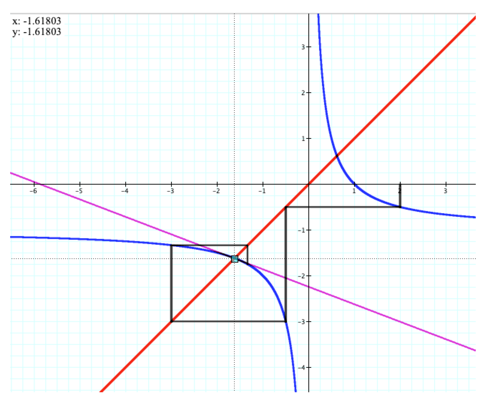
Note that although the case a = 1 and b = −1 (just explored using three instruments) satisfies the relation a + b = 0 (the first one that might come to mind), the case a = −1 and b = 1 yields Lucas numbers with alternating signs, 1, 2, −1, 3, −4, 7, −11, 18, and (not surprisingly) results in the convergence of the corresponding ratios to the negative Golden Ratio. This process of convergence of the ratios $r_n=\frac{f_{n+1}}{f_n}$, satisfying a non-linear modification $r_n=-1+\frac{1}{r_{n-1} }$ of linear Equation (7), to the negative Golden Ratio (rather than to a three-cycle) is shown graphically in Figure 17 through a staircase diagram. The staircase, by bouncing down/left to up/right between the graphs of the functions $y=-1+\frac{1}{x}$ and $y=x$, approaches the value $x=\frac{-1-\sqrt{5}}{2}$. This value is the attracting fixed point of the hyperbolic map $x\to -1+\frac{1}{x}$ because the absolute value of the slope of the tangent line to the graph of the map at the point $x=\frac{-1-\sqrt{5}}{2}$ (unlike $x=\frac{-1+\sqrt{5}}{2}$—the second fixed point of the map) is smaller than one.

In order to find all three-cycles which, just as the triple (2, 0.5, −1), attract the ratios $f_{n+1}/f_n$, Equation (7) can be re-written in the form $r_n=a+\frac{b}{r_{n-1}}$ where $r_n=\frac{f_{n+1}}{f_n}$, $r_1=2,$ so that the relation $r_1=r_4$ expressed in terms of a and b provides the relation sought. In doing so, one can write $r_2=a+b/2, r_3=a+\frac{b}{a+b/2}, r_4=a+\frac{b}{a+\frac{b}{a+b/2}} .$ Using Wolfram Alpha (Figure 18), one can solve the continued fraction equation $a+\frac{b}{a+\frac{b}{a+b/2}}=2$ yielding b = 4 − 2a, a trivial case of a cycle of any length (consisted of twos—initial values), and $b=-a^2$—the non-trivial case of a three-cycle formed by the ratios $r_n=\frac{f_{n+1}}{f_n}$. For example, when $r_1=2$ we have $r{ }_2=a-\frac{a^2}{2}=\frac{2a-a^2}{2}, r_3=a-\frac{a^2}{\frac{2a-a^2}{2}}=\frac{a^2}{a-2}$, $r_4=a-\frac{a^2}{\frac{a^2}{a-2}}=2$ so that ${\left(2, \frac{2a-a^2}{2}, \frac{a^2}{a-2}\right)|}_{a=1}=\left(2,\frac{1}{2},-1\right)$.

Alternatively, as part of computational triangulation, the relation $r_1=r_4$ can be graphed (Figure 19) using the Graphing Calculator (substituting x for a and y for b). This graphing can be considered as triangulation within a method (of finding three-cycles) demonstrating that the point (−1, 1), which corresponds to a possible accidental misprint in a spreadsheet formula, belongs to the parabola $b=-a^2.$ Likewise, the point (a, b) = (1.290569415, −1.665569415) selected by the cursor on the parabola $b=-a^2$ and then plugged into the spreadsheet of Figure 20 to model the behavior of the ratios $\frac{f_{n+1}}{f_n}$ in Equation (7), can be used to triangulate the phenomenon of convergence to another three-cycle (2, 0.45778471, −2.3477553).

Computational triangulation helps teacher candidates appreciate relationship that exists between two types of knowledge—experimental and theoretical. As one of the author’s students noted: “It is important to make connections between experimental and theoretical knowledge in order to deepen one’s understanding of the material. The experimental portion came when picking points off of the theoretically found parabola [see Figure 18 and Figure 19] and plugging them into the spreadsheet [see Figure 20]. It was also hypothesized that the equation relating variables a and b for a cycle of 3 would also be present in any cycle that was a multiple of 3. This was tested experimentally using the spreadsheet and Maple software [see Figure 21]”.

Finally, using Maple (Figure 21) to solve equations with continued fractions, computational triangulation can be extended to generate parabolic loci of the cycles of lengths four, five and six, all of the form

$$b=-\mu a^2, \mu >0$$

(8)

and all including the trivial cycle b = 4 − 2a. Furthermore, as part of computational triangulation, one can see (Figure 21) that the cycles of length six do include cycles of length three. In addition, one can see that beginning from cycles of length five, the loci of the cycles consist of more than one parabola, all such parabolas sharing the origin of the plane of parameters as their common vertex. It is this activity that another teacher candidate described as follows: “In this project, spreadsheets were used first to observe convergence. Graphs clearly depicted if a coordinate point (a, b) converged to a specific value, helping students to visually understand convergence. Additionally, the graphing calculator was used to graph the cubic equation obtained from Maple when working with continued fractions. The cubic equation about a^2/b contained three parabolas, which students can visualize; graphing the cubic equation also allows students to see all points on the parabolas that result in cyclic behavior for a particular difference equation.” For more information about the behavior of generalized Golden Ratios see [43].

8. Conclusions

The word triangulation, having origin in mathematics, is commonly used in social sciences toward achieving rigor as the unity of theory and method [12]. In mathematics, since the time of Euclid—the most prominent mathematician of the 3rd century BC—methods of proof have been continuously perfected under the banner of rigor, leading to more and more abstract mathematics. Nonetheless, as Pierpont [49] (p. 23) put it, achieving absolute rigor “will be a sign that the race of mathematicians has declined”. In the era of standards-based mathematics education, many fundamental ideas, otherwise intrinsically abstract, can nonetheless be well explained contextually, by using concrete problems. This points to the importance of concrete problems as pedagogical tools in the teaching of mathematics. Concreteness makes a student confident in the usefulness of material to be studied, seeing a logical connectivity of mathematical ideas and their successive reliance on each other. Such a pedagogical approach helps a student of the subject matter “to recognize a mathematical concept in, or to extract it from, a given concrete situation” [50] (pp. 100–101).

With this in mind, the paper started with the problem of putting candies on plates in which the recursive character of addition guided by Fibonacci-like numbers was hidden behind a homely action with the intent of being revealed later to support the programming of a computational environment. Originally, the problem (Brain Teaser) served as the background for the introduction of four computational triangulation techniques; although they were not needed for the problem to be solved. However, from the point of view of mathematics education, computational approaches to problem solving are better understood when hidden mathematical elements of a problem are extracted from the context in order to be used as building blocks of computational algorithms. At that point, several mathematical ideas were discussed including the Golden Ratio, Binet’s formula, parametric difference equations, and, eventually, continued fractions.

The use of the Graphing Calculator made it possible to construct a staircase diagram demonstrating the geometric meaning of multiple phenomena. These included two types of fixed points that the graph of a function may have—attracting and repealing—when crossed by the identity line y = x; visual recognition of which type the point belongs to in terms of the slope that the tangent line to the graph at a fixed point has and the angle it forms with the identity line. In that way, computational triangulation enables a fairly intelligible demonstration of rather complicated mathematical ideas, something that is especially beneficial for the mathematics education of teachers.

It was shown how a peculiar outcome of an accidental misprint in carrying out computational triangulation when attended with epistemic care can open a window to new mathematical ideas stemming from classic concepts to be further explored using the same computational tools that were used to triangulate conventional outcomes. The new (i.e., not commonly known in mathematics education or even previously in mathematics) concept discussed in the paper included the so-called generalized Golden Ratio in the form of a string of numbers the length of which, depending on the value of $\mu$ in relation to (8), can be as long as one wishes.

The ideas of this paper were motivated by the author’s work with teacher candidates of the United States and Canada using various tools of technology in the courses of different degrees of mathematical complexity. The notion of computational triangulation made it possible to carefully differentiate the presentation of mathematics between primary and secondary levels by either exiting the computational train at the appropriate place or allowing it to continue moving full speed ahead demonstrating the true meaning of the motto “mathematics unlimited” [51]. The approach made it possible to demonstrate to both populations of future teachers that in the age of standards-based teaching and learning, digital computations open multiple windows to mathematical ideas that, using one more time, in the conclusion, quotations from different parts of the paper, “stimulate an inquisitive attitude and reasoning among students” [22] (p. 37), “enhance the potential for teachers to make mathematics interesting” [19] (p. 9) thus allowing for “virtual worlds that are unconstrained by physical realities” [29] (p. 21), “in which the curiosity of students can lead to rich mathematical discoveries” [21] (p. 9). Although the paper is limited to K-12 teacher education, all these affirmational quotes are applicable to the use of computational triangulation at the tertiary level of mathematics education as well.

References

- Campbell, D.T. A Study of Leadership among Submarine Officers; Ohio State University Research Foundation: Columbus, OH, USA, 1953. [Google Scholar]
- Campbell, D.T. From Description to Experimentation: Interpreting Trends as Quasi-Experiments. In Problems in Measuring Change; Harris, C.W., Ed.; University of Chicago Press: Madison, WI, USA, 1963; pp. 212–242. [Google Scholar]
- Webb, E.J.; Campbell, D.T.; Schwartz, R.D.; Sechrest, L. Unobtrusive Measures; Rand McNally: Chicago, IL, USA, 1966. [Google Scholar]
- Boaler, J.; Ball, D.L.; Even, R. Preparing Mathematics Education Researchers for Disciplined Inquiry: Learning from, in, and for Practice. In Second International Handbook of Mathematics Education; Bishop, A.J., Clements, M.A., Keitel, C., Kilpatrick, J., Leung, F.K.S., Eds.; Springer International Handbooks of Education, Springer: Dordrecht, The Netherlands, 2003; Volume 10, pp. 491–521. [Google Scholar]
- Sharma, S. Qualitative approaches in mathematics education research: Challenges and possible solutions. Educ. J. 2013, 2, 50–57. [Google Scholar] [CrossRef]
- Löwe, B.; van Kerkhove, B. Methodological Triangulation in Empirical Philosophy (of Mathematics). In Advances in Experimental Philosophy of Logic and Mathematics; Aberdein, A., Inglis, M., Eds.; Bloomsbury Publishing: London, UK, 2019; pp. 15–37. [Google Scholar]
- Abramovich, S. Advancing the concept of triangulation from social sciences research to mathematics education. Adv. Educ. Res. Eval. 2022, 3, 201–217. [Google Scholar] [CrossRef]
- Wing, J.M. Computational thinking. Comm. ACM 2006, 49, 33–35. [Google Scholar] [CrossRef]
- Freudenthal, H. Weeding and Sowing; Kluwer: Dordrecht, The Netherlands, 1978. [Google Scholar]
- Harrison, J. Formal proof—Theory and practice. Not. Am. Math. Soc. 2008, 55, 1395–1406. [Google Scholar]
- McFee, G. Triangulation in research: Two confusions. Educ. Res. 1992, 34, 215–219. [Google Scholar] [CrossRef]
- Denzin, N.K. The Research Act in Sociology: The Theoretical Introduction to Sociological Methods; Butterworth: London, UK, 1970. [Google Scholar]
- National Council of Teachers of Mathematics. Principles to Actions: Ensuring Mathematical Success for All; National Council of Teachers of Mathematics: Reston, VA, USA, 2014. [Google Scholar]
- Char, B.W.; Geddes, K.O.; Gonnet, G.H.; Leong, B.L.; Monagan, M.B.; Watt, S.M. Maple V Language Reference Manual; Springer: New York, NY, USA, 1995. [Google Scholar]
- Power, D.J. A Brief History of Spreadsheets, DSSResources.COM. 2000. Available online: http://dssresources.com/history/sshistory.html (accessed on 7 February 2023).
- Avitzur, R. Graphing Calculator [Version 4.0]; Pacific Tech: Berkley, CA, USA, 2011. [Google Scholar]
- Denzin, N.K. Triangulation. The Blackwell Encyclopedia of Sociology; Ritzer, G., Ed.; Blackwell Publishing: Malden, MA, USA, 2007; Volume 10, pp. 5075–5080. [Google Scholar]
- Saukko, P. Doing Research in Cultural Studies: An Introduction to Classical and New Methodological Approaches; Sage: London, UK, 2003. [Google Scholar]
- National Curriculum Board. National Mathematics Curriculum: Framing Paper. Author: Australia. 2008. Available online: http://www.acara.edu.au/verve/_resources/National_Mathematics_Curriculum_-_Framing_Paper.pdf (accessed on 7 February 2023).
- Ontario Ministry of Education. The Ontario Curriculum, Grades 1–8, Mathematics (2020). 2020. Available online: http://www.edu.gov.on.ca (accessed on 7 February 2023).
- Western and Northern Canadian Protocol. The Common Curriculum Framework for Grades 10–12 Mathematics. 2008. Available online: http://www.bced.gov.bc.ca/irp/pdfs/mathematics/WNCPmath1012/2008math1012wncp_ccf.pdf (accessed on 7 February 2023).
- Felmer, P.; Lewin, R.; Martínez, S.; Reyes, C.; Varas, L.; Chandía, E.; Dartnell, P.; López, A.; Martínez, C.; Mena, A.; et al. Primary Mathematics Standards for Pre-Service Teachers in Chile; World Scientific: Singapore, 2014. [Google Scholar]
- Advisory Committee on Mathematics Education. Mathematical Needs of 14–19 Pathways; The Royal Society: London, UK, 2007. [Google Scholar]
- Ministry of Education Singapore. Mathematics Syllabuses, Secondary One to Four; The Author: Curriculum Planning and Development Division. 2020. Available online: https://www.moe.gov.sg/-/media/files/secondary/syllabuses/maths/2020-express_na-maths_syllabuses.pdf?la=en&hash=95B771908EE3D777F87C5D6560EBE6DDAF31D7EF (accessed on 7 February 2023).
- Department of Basic Education. Mathematics Teaching and Learning Framework for South Africa: Teaching Mathematics for Understanding; Private Bag: Pretoria, South Africa, 2018.
- Common Core State Standards. Common Core Standards Initiative: Preparing America’s Students for College and Career. 2010. Available online: http://www.corestandards.org (accessed on 7 February 2023).
- Conference Board of the Mathematical Sciences. The Mathematical Education of Teachers II; The Mathematical Association of America: Washington, DC, USA, 2012. [Google Scholar]
- Association of Mathematics Teacher Educators. Standards for Preparing Teachers of Mathematics. 2017. Available online: amte.net/standards (accessed on 7 February 2023).
- Wing, J.M. Research Notebook: Computational Thinking—What and Why. Link Mag. 2011, 6, 20–23. Available online: https://people.cs.vt.edu/~kafura/CS6604/Papers/CT-What-And-Why.pdf (accessed on 7 February 2023).
- Arnheim, R. Visual Thinking; University of California Press: Berkeley, CA, USA; Los Angeles, CA, USA, 1969. [Google Scholar]
- Vygotsky, L.S. Mind in Society; Harvard University Press: Cambridge, MA, USA, 1978. [Google Scholar]
- Gershenfeld, N. Fab: The Coming Revolution on Your Desktop—From Personal Computers to Personal Fabrication; Basic Books: New York, NY, USA, 2005. [Google Scholar]
- Beghetto, R.A.; Kaufman, J.C.; Baer, J. Teaching for Creativity in the Common Core Classroom; Teachers College Press: New York, NY, USA, 2015. [Google Scholar]
- Koshy, T. Fibonacci and Lucas Numbers with Applications; Wiley: New York, NY, USA, 2001. [Google Scholar]
- Catalan, E. Notes sur la Théorie des Fractions Continues et sur Certaines Séries. In Mémoires de L’Académie Royale des Sciences, des Lettres et des Beaux-Arts de Belgique, Tome XLV; Hayez, F.F., Ed.; Imprimeur de L’Académie Royale: Bruxelles, Belgique, 1884. [Google Scholar]
- Knuth, D.E. The Art of Computer Programming, Fundamental Algorithms; Addison Wesley: Reading, MA, USA, 1977; Volume 1. [Google Scholar]
- Wells, D. The Penguin Dictionary of Curious and Interesting Numbers; Penguin Books: Middlesex, UK, 1986. [Google Scholar]
- Weisstein, E.W. CRC Concise Encyclopedia of Mathematics; Chapman & Hall/CRC: Boca Raton, FL, USA, 1999. [Google Scholar]
- Apostol, T.M. Calculus: One-variable Calculus, with Introduction to Linear Algebra; Wiley: Hoboken, NJ, USA, 1967; Volume 1. [Google Scholar]
- McCallum, W. Mathematicians and Educators: Divided by a Common Language. In Mathematics in Undergraduate Study Programs: Challenges for Research and for the Dialogue between Mathematics and Didactics of Mathematics; Report No. 56/2014; Mathematicsches Forschungsinstitut Oberwolfach: Oberwolfach, Germany, 2015; pp. 48–49. [Google Scholar] [CrossRef]
- Kilpatrick, J. Reformulating: Approaching Mathematical Problem Solving as Inquiry. In Posing and Solving Mathematical Problems: Advances and New Perspectives; Felmer, P., Pehkonen, E., Kilpatrick, J., Eds.; Springer: New York, NY, USA, 2016; pp. 69–81. [Google Scholar]
- Béguin, P.; Rabardel, P. Designing instrument-mediated activity. Scand. J. Inform. Syst. 2000, 12, 173–190. [Google Scholar]
- Abramovich, S.; Leonov, G.A. Revisiting Fibonacci Numbers Through a Computational Experiment; Nova Science Publishers: New York, NY, USA, 2019. [Google Scholar]
- Sloane, N.J.A. The On-Line Encyclopedia of Integer Sequences. Available online: http://www.research.att.com/~njas/sequences/ (accessed on 7 February 2023).
- Matijasevic, J.V. Diophantine representation of enumerable predicates. Math. USSR—Izvestiya 1971, 5, 1–28. [Google Scholar] [CrossRef]
- Hilbert, D. Mathematical problems (Lecture delivered before the International Congress of Mathematicians at Paris in 1900). Bull. Am. Math. Soc. 1902, 8, 437–479. [Google Scholar] [CrossRef]
- Langtangen, H.P.; Tveito, A. How Should We Prepare the Students of Science and Technology for a Life in the Computer Age? In Mathematics Unlimited—2001 and Beyond; Engquist, B., Schmid, W., Eds.; Springer: New York, NY, USA, 2001; pp. 809–825. [Google Scholar]
- Kaput, J.J. Technology and Mathematics Education. In Handbook of Research on Mathematics Teaching and Learning; Grouws, D.A., Ed.; Macmillan: New York, NY, USA, 1992; pp. 515–556. [Google Scholar]
- Pierpont, J. Mathematical rigor, past and present. Bull. Amer. Math. Soc. 1928, 34, 23–53. [Google Scholar] [CrossRef] [Green Version]
- Pólya, G. Mathematical Discovery: On Understanding, Learning and Teaching Problem Solving; Wiley: New York, NY, USA, 1965; Volume 2. [Google Scholar]
- Engquist, B.; Schmid, W. (Eds.) Mathematics Unlimited—2001 and Beyond; Springer: New York, NY, USA, 2001. [Google Scholar]
Figure 1.
Solving Equation (1) by Wolfram Alpha.
Figure 2.
Solution to the Brain Teaser.
Figure 3.
Graphical representations of Equation (1) and its solution.
Figure 4.
Solving Equation (1) within a two-dimensional spreadsheet.
Figure 5.
Using Wolfram Alpha in multiplying two geometric series.
Figure 6.
Solving the Brain Teaser by using Binet’s formula in spreadsheet programming.
Figure 7.
Computerization of the “well-ordering principle”.
Figure 8.
Graphical solution of reformulated Brain Teaser.
Figure 9.
Using Maple in solving Equation (3).
Figure 10.
Using Wolfram Alpha in solving Equation (3).