Article

Deep Web Search Interface Identification: A Semi-Supervised Ensemble Approach

School of Mathematics & Statistics, Central South University, Changsha 410075, China
*
Author to whom correspondence should be addressed.
Information 2014, 5(4), 634-651; https://doi.org/10.3390/info5040634
Submission received: 30 October 2014 / Revised: 24 November 2014 / Accepted: 28 November 2014 / Published: 1 December 2014
(This article belongs to the Section Information and Communications Technology)

Abstract

:
To surface the Deep Web, one crucial task is to predict whether a given web page has a search interface (searchable HyperText Markup Language (HTML) form) or not. Previous studies have focused on supervised classification with labeled examples. However, labeled data are scarce, hard to get and requires tedious manual work, while unlabeled HTML forms are abundant and easy to obtain. In this research, we consider the plausibility of using both labeled and unlabeled data to train better models to identify search interfaces more effectively. We present a semi-supervised co-training ensemble learning approach using both neural networks and decision trees to deal with the search interface identification problem. We show that the proposed model outperforms previous methods using only labeled data. We also show that adding unlabeled data improves the effectiveness of the proposed model.

1. Introduction

The Deep Web (also called the Invisible Web and the Hidden Web) refers to a part of World Wide Web content that is different from the Surface Web, which can be crawled and easily indexed by traditional search engines [1]. The vast information of the Deep Web is located behind specific web search interfaces, usually in the form of HTML forms [2], and can be surfaced only by formulating a search query on such interfaces [3]. Understanding the search interfaces [4], sampling the web databases [5], classification and integration of web sources [6,7] are the key problems that often arise in mining the Deep Web.
In dealing with the above-mentioned problems, one usually assumes that search interfaces are often identified and ready to use. However, identifying whether a web page contains search interfaces or not is still challenging and non-trivial to date. If the scale of the deep web under investigation is small, we could manually judge and collect the search interfaces, as was done in [8,9]. However, this method will not work for the real Deep Web, which is estimated to be 500 times larger than the Surface Web [1].
The search interface identification process has to be automatic. In a machine learning environment, a binary classifier is needed to differentiate searchable interfaces from non-searchable ones. The past decade has seen various approaches to identify search interfaces, including decision trees [2], adaptations of random forests [10] and other combinations of machine learning techniques [11]. Regardless of which learning algorithm is used, most identification approaches are supervised and have to face the problem of the scarcity of labeled data.
In this paper, we introduce a semi-supervised search interface identification approach, which is different from most previous supervised-based classification techniques [2,10,12,13] and the semi-supervised proposed method in [14]. In our approach, two-base classifiers, namely neural networks and decision trees, are trained alternatively to obtain additional diversity data from unlabeled examples. We then use the unlabeled diversity data to increase the diversity of the base classifiers in the ensemble. Experiments show that our proposed approach, SSCTE (semi-supervised co-training ensemble) outperforms state-of-the-art supervised classifiers, such as K Nearest Neighbours (KNN), Support Vector Machines (SVM) boosting and random forests, in most cases.
As a second contribution, we provide a group of search interface identification datasets for the Deep Web research community. Previous research mainly adopted the University of Illinois at Urbana-Champaign (UIUC) Web Integration Repository [15] in their experiments, but the number of examples actually used in related experiments varies. This is because some of the URLs in the datasets are out-of-date and no longer available, and thus, their experiments might not be verified. This inspired us to create a repository of our own and to make it public with both URLs and the downloaded HTML forms. Our datasets can be downloaded from the web site (https://github.com/whcsu/sscte/) or will be sent upon request. It is by far the largest dataset available in terms of labeled search interface examples.
The rest of the paper is organized as follows. Section 2 overviews related work in search interface identification and semi-supervised ensemble learning. In Section 3, we propose a novel search interface identification approach based on semi-supervised co-training ensembles. Th experimental setup and result analysis are described in Section 4. Finally, in Section 5, we conclude the paper.

2. Related Work

In this section, we briefly review previous studies on search interface identification and take a glimpse at semi-supervised classification and semi-supervised ensembles in particular. Later on, we shall develop a novel search interface identification algorithm within the semi-supervised ensemble learning framework.

2.1. Search Interface Identification

The search interface identification problem can be stated formally in the following way: given a set of web pages W A , find W S W A that contains searchable interfaces. Since HTML forms constitute a large majority of search interfaces on the Deep Web, most studies focus on HTML form-based search for identification.
A search form, through which a query can be issued by modifying the controls and then submitted for further processing, is usually a section of an HTML file that begins with a < f o r m > tag and ends with a < / f o r m > tag. A typical search form on www.arxiv.org and its corresponding source code are shown in Figure 1 and Figure 2.
Figure 1. Arxiv search interface: a simple search form.
Information 05 00634 g001
Figure 2. Arxiv search interface: HTML source code.
Information 05 00634 g002
To automatically identify the search interfaces among a vast amount of HTML forms, a number of supervised machine learning algorithms have been proposed, and these methods fall into two categories: pre-query and post-query. Pre-query algorithms use a form classifier to judge an HTML file according to the form features in the interface. Post-query methods identify the form searchability by submitting queries through HTML forms in the interface, and a decision is made based on the returned result pages.
Cope et al. [2] proposed a pre-query approach with the C4.5 decision tree as the learning algorithm to classify them. This method was further developed by [11,12], but far less features were used. Shestakov [13] also applied decision tree algorithms in identifying search interfaces, but they divided all HTML forms into two groups based on the number of visible controls and implemented two separate binary classifiers for classification. They demonstrated that such separation improves the system accuracy. Ye et al. [10] extended the random forest algorithm by applying a weighted feature selection during the building of individual tree classifiers. Wang et al. [16] proposed a hierarchical framework, which used an ontology in the web page classifier and in the form content classifier, while a C4.5 decision tree in the form structure classifier. Marin-Castro et al. [17] created eight heuristic rules based on extensive heuristic analysis to discriminate non-searchable from searchable HTML forms.
Bergholz and Childlovskii [18] gave an example of the post-query approach. They constructed a form analyzer using different heuristics, such as the length of the input field, the presence or absence of password protection, to identify whether a form was queryable. They then applied a query prober to manage the automatic form filling and decided the usefulness of the form according to the results of probing. Lin and Zhou [19] studied simple search interfaces with only one single input field, but could accept multiple search keywords of different attributes and provided a search interface probing strategy based on the query words’ hit rate and the reappearance frequency of the query words in the result pages.
From the above, we may notice that as the post-query approach requires automatic filling of HTML forms, which is very challenging for HTML forms with multiple input controls, it has found very limited applications so far. Additionally, due to the same reason, pre-query approaches dominate today’s search interface identification solutions.
Previous search interface identification approaches have demonstrated the power of supervised classification algorithms. However, in building supervised classifiers, we often face the problem of scare labeled examples together with a vast amount of unlabeled data. As semi-supervised learning (SSL) methods can exploit both labeled and unlabeled data to obtain a higher accuracy, we might turn to SSL for help [20,21].

2.2. Semi-Supervised Ensemble Learning

SSL falls between unsupervised learning (without any labeled examples) and supervised learning (with labeled examples only) [20]. In a semi-supervised classification framework, l labeled examples L = { x 1 , , x l } and u unlabeled examples U = { x l + 1 , ..., x l + u } are given and exploited together in training to find a good classifier with improved accuracy. SSL algorithms usually work in the following way: first, a classifier is trained on L, and an initial hypothesis H is obtained; then, H is used to classify the examples in U; the examples with high confidence are labeled, added to L and deleted from U; this process is iterated for a fixed number of times or stopped when U becomes empty.
Semi-supervised ensemble learning (also called semi-supervised multiple classifier systems, semi-supervised learning by disagreement) [22,23] is a kind of SSL algorithm that exploits unlabeled data collaboratively to increase the performance of the ensemble. Since highly diverse base classifiers are the key to the success of ensemble systems [24,25], different strategies in supervised ensemble learning, such as bagging [26], boosting [27] and random subspace [28], are extended to the semi-supervised framework to obtain a higher ensemble diversity and, hence, a higher classification accuracy.
Semi-supervised MarginBoost (SSMBoost), proposed in [29], generalized AdaBoost [30] to semi-supervised classification by redefining the margin notion to include unlabeled data. The same as SSMBoost, Adaptive Semi-Supervised Ensemble (ASSEMBLE) [31] also adopted the MarginBoost notation for both labeled and unlabeled data. The major difference is that they assign pseudo-classes to the unlabeled data in constructing the ensembles. SemiBoost [32] exploited both the clustering assumption and the large margin criterion. It also used the pairwise similarity measurements to guide the selection of unlabeled examples at each iteration. Different from the above boosting-based semi-supervised ensembles, co-forest [33] incorporated random forest in the semi-supervised framework and demonstrated the strength of bagging and random space method in computer-aided medical diagnosis.

3. A Semi-Supervised Co-Training Ensemble

Our proposed method addresses the search interface identification problem by turning it into an ensemble learning problem using both labeled and unlabeled data. As the key to successful ensemble learning methods is to construct individual base classifiers that are as diverse as possible, thus increasing the ensemble’s diversity, a strategy of varying both the training data and the base classifier themselves is adopted in the proposed algorithm.
In our approach, the most popular methods to achieve diversity from labeled training data obtained through resampling techniques, such as bagging and random subspace, are applied, and these methods will be detailed in the first part of this section. Later on, we focus on how to obtain further diversity from unlabeled training examples, which is also the major novelty of the proposed algorithm. Besides the data diversity, we also consider the diversity caused by the base classification algorithms themselves and discuss how to combine the outputs of these base classifiers effectively. Finally, we present our semi-supervised co-training ensemble (SSCTE) learning algorithm.

3.1. Diversity Generation from Data

In the proposed algorithm, we exploit both bagging and random subspace methods in training the base classifiers, as is done in co-forest [33]. In bagging [26], base classifiers are trained on a bootstrapped example of the original training set. In random subspace (attribute bagging) [28], various feature subsets of the original data are created by sampling the whole feature set without replacement. Additionally, training data with different bootstrapped versions and subsets of features are used to train diverse base classifiers.
However, when a large amount of unlabeled data is available, diversity obtained from labeled data alone is not enough, and we should try to gain further diversity from the unlabeled examples, as well.
Melville et al. [34] introduced a supervised ensemble learning algorithm, called DEcoratE, which artificially generates new wrongly-labeled examples (termed diversity data) and merges the diversity data with the training data to train new base classifiers. Their experiments show that the diversity data did increase the diversity among the base classifiers and, therefore, improved the classification accuracy. In this paper, instead of obtaining diversity data from labeled training examples, we want to use the information from the vast amount of unlabeled data to create it.
First, a base classifier trained on the labeled data is applied to make predictions on the unlabeled data. Then, unlabeled examples with a highly confident prediction probability are selected. These highly confident examples will be misclassified deliberately (i.e., given class labels opposite of the predictions of the base classifier) and will be used for the creation of the diversity data pool. The total number of examples to be selected is specified as a fraction, D f r a , of the original training set size. The process of diversity data creation is shown in the following Algorithm 1:
Algorithm 1 Diversity data creation.
Input: L = { x i } i = 1 l , labeled data
    U = { x i } i = l + 1 l + u , unlabeled data
   BaseLearn, base learning algorithm
   pconf, confidence probability threshold
   Dfra, factor that determines number of diversity data.
Procedure:
  1: train BaseLearn on L;
  2: use BaseLearn to calculate class probability pi, for example ui in U;
  3: label ui with class opposite to the prediction if its pi > pconf;
  4: add all uis in Steps 2 and 3 to the diversity data pool;
  5: select Dfra most confident examples in the pool to form D.
Output: D, diversity data

3.2. Diversity Obtained from Base Classification Algorithms

Unstable classification algorithms (i.e., a small change in the training set can lead to a remarkable change in the produced model), such as neural networks and decision trees, are good candidates for base classifiers in ensemble learning [24,26]. Most supervised or semi-supervised ensemble learning algorithms only consider one kind of base classification algorithm, either decision trees [33,35,36] or neural networks [37].
As neural networks and decision trees classifiers are drastically different in nature, and they may make different (uncorrelated) errors on the same examples, i.e., examples misclassified by neural networks might be corrected by decision trees and vice versa. This build-in complementary mechanism of the base classifiers will increase the base classifiers’ diversity and therefore should improve the classification accuracy of the ensemble on the whole.
Thus, instead of using only one kind of base learning algorithm, we use both neural networks and decision trees as the base algorithms, and these two kinds of classifiers are trained alternatively in the whole process, as is done in the co-training algorithm [38]. This is why we call the algorithm semi-supervised co-training ensemble.

3.3. Aggregating the Base Classifiers

In ensemble learning algorithms, different base classifiers usually have different prediction capabilities. Classifiers that have high predicative power should be given higher weights. Thus, in SSCTE, we adopt a weighted majority mechanism in combing the base classifiers, and the weights of base classifiers are based upon their performance on the so-called out-of-bag data.
In SSCTE, each base classifier is constructed using a different bootstrap sample from the original labeled data plus some diversity data. About 1 / 3 of the labeled data are left out of the bootstrap sample and not used in the i-th iteration. The out-of-bag (OOB) data generated in the i-th iteration are used to examine the performance of the i-th base classifier. Additionally, the resulting OOB prediction accuracy o o b i will be used to calculate the weight of the i-th base classifier w [ i ] , according to the following formula:
w [ i ] = 1 , o b b i = o o b m a x ; ( o o b m a x o o b i ) ( o o b m a x o o b m i n ) , o o b m i n < o b b i < o o b m a x ; 0 , o o b i m a x ( o o b m i n , 0 . 5 ) .
where o o b m a x , o o b m i n are the maximum and minimum values among all OOB accuracy values o o b i s, respectively.

3.4. The Algorithm

In SSCTE (see Algorithm 2), a semi-supervised ensemble is generated iteratively.
Algorithm 2 A semi-supervised co-training ensemble (SSCTE) learning algorithm.
Input: L, U, pconf, Dfra
  F, feature space f1, … , fp of examples in L
  Fi, subset of features of F used in the i-th iteration
  BaseTree, decision tree learning algorithm
  BaseNet, neural net learning algorithm
  Di, diversity data obtained in the i-th iteration using Algorithm 1
  K, number of iterations
Initialization: C = Ø; D0 = Ø
 1: for ( i = 1 ; i K ; i + + ) do
 2:  generate a bootstrapped sample Li of L
 3:  if i is odd then
 4:    draw Fi from F using random subspace to form L i from Li
 5:    use C i = B a s e T r e e ( L i + D i 1 ) to create diversity data Di in U
 6:  end if
 7:  if i is even then
 8:    use C i = B a s e N e t ( L i + D i 1 ) to create diversity data Di in U
 9:    use Ci to predict OOB data and record the prediction accuracy oobi
10:    U = UDi, remove the diversity data from U
11:  end if
12:  if U is empty then
13:    break
14:  end if
15:   C = C C i
16: end for
17: calculate weights w[i]s for all classifiers based on their oobis according to formula (1)
Output: the learning ensemble C. In prediction, a sample (x, y) is assigned with class label y* as the one receiving the weighted majority of the votes:
y * = arg max y C i C w [ i ] * C i ( x , y )
Initially, a bootstrapped sample is generated from the original labeled dataset. In each iteration, the current base classifier is trained on a different bootstrapped dataset plus some diversity data created by the previous base classifier using Algorithm 1. The diversity data are then removed from the unlabeled data. This iterative process continues until the unlabeled data become empty or the iteration number condition is reached. Finally, base classifiers trained in all iterations are combined together using weighted majority voting.

4. Experimental Results

In this paper, we are going to classify a held out test set using the SSCTE algorithm learned on a training set consisting of both labeled and unlabeled examples. We first describe the Deep Web search interface dataset used in the experiments and then discuss two evaluation metrics and the statistic tests used. Finally, we present the experiment results.

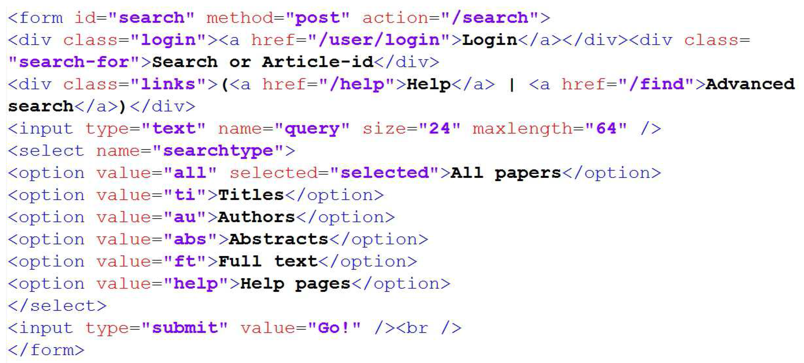
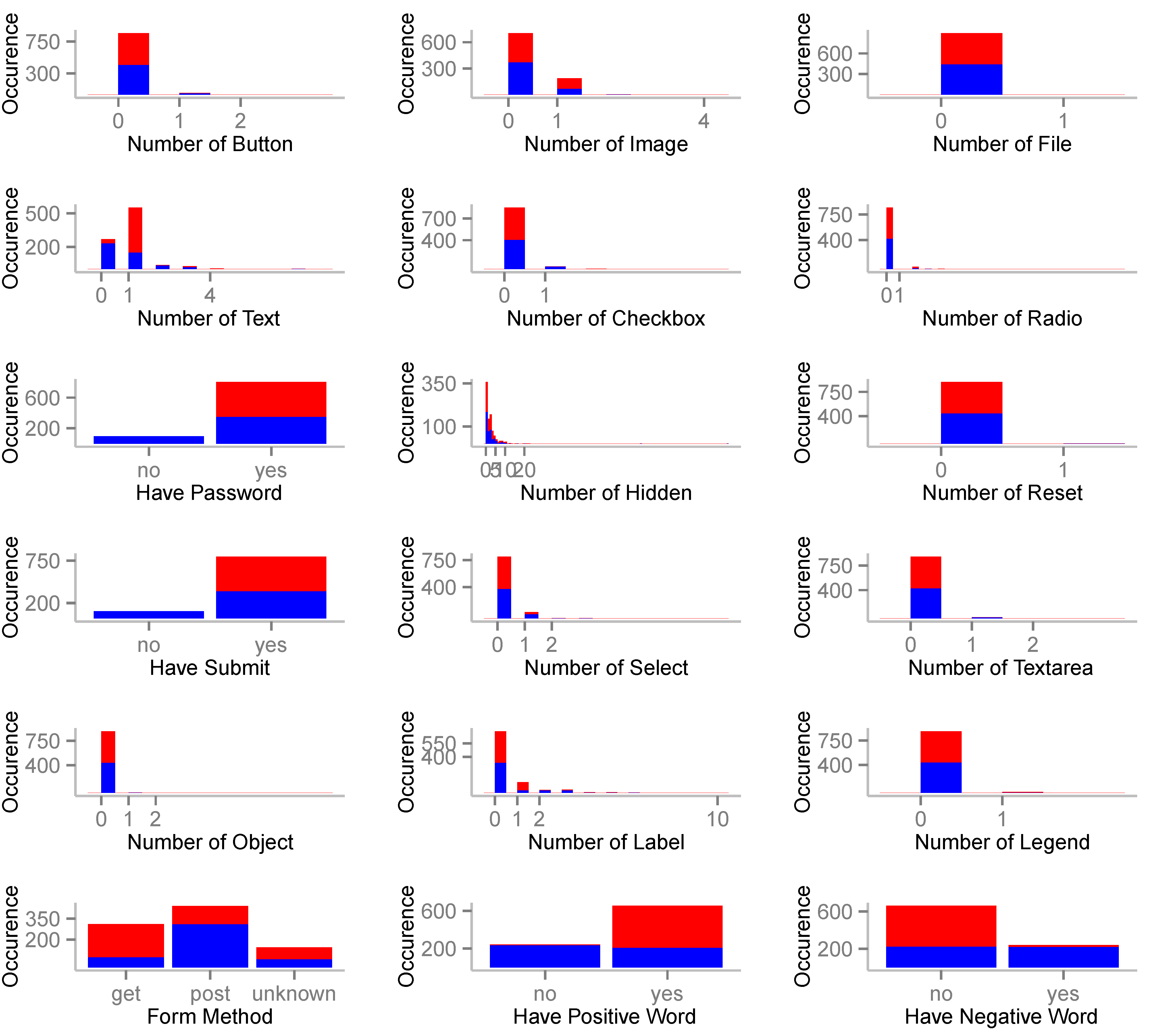
4.1. Dataset Description

We evaluate the performance of our algorithm on real-world search interface datasets in Deep Web mining. The most related dataset used in previous research is the UIUC Web Integration Repository and was provided by [15] in 2004. However, as time goes by, many web links out of the 447 query interfaces in the repository have become broken, and some domain names have even disappeared. Consequently, it is not adequate to still compare the algorithms’ performance based on the outdated UIUC dataset. Thus, in this study, we only consider the recently collected dataset by the authors with both the original HTML forms and processed data that are publicly available. It is by far the largest search interface dataset used in similar research and can be downloaded from https://github.com/whcsu/sscte/. The Comma-Separated Values (CSV) and Attribute-Relation File Format (ARFF) files of the dataset are also available upon request. A brief description of the dataset is detailed in Table 1.
Table 1. Dataset used in the experiments.
Search FormsNon-Search Forms
DMOZ labeled451446
DMOZ unlabeled18,624
The dataset contains 897 labeled examples and 18,624 unlabeled examples and is extracted by crawling some of the web links indexed in the largest web directory www.DMOZ.org during the period April 2011, and March 2012. The distribution for the DMOZ dataset varies, ranging from general sites, academic sites, recreation sites to social sites and science sites.
An important step in classifying search forms from non-search forms is to characterize the HTML forms embedded in the deep web HTML files. This is usually done through extracting certain features within the forms. As shown in [2], features, such as the numbers of “text” INPUT control and SELECT control are good indicators of the form searchability. Suggested in [10], FORM attributes, such as “method” and “action”, are also considered in our research. These features are extracted from the form element or control structures and will be called “structural features” in our research. One may notice that in Figure 2, the word “search” occurs five times within the form body, and such semantically “positive” words help a human to determine the form searchability. Generally, LABEL name, FORM action URL and textual contents within the form are of great semantical importance and they become “semantical features” in our extracted feature set.
In our approach, we have extracted 18 features to characterize Deep Web search forms. Statistical distributions of all 18 features in search and non-search forms are shown in the following Figure 3, where feature occurrences of search forms and non-search forms are indicated by red and blue colors, respectively.
Figure 3. Feature distributions in HTML forms.
Information 05 00634 g003

4.2. Evaluation Metrics and Statistical Tests

We use the following abbreviations for the ease of explanation: P (# positive, i.e., search interface examples), N (# negative, i.e., non-search interface examples), TP (# true positives), TN (# true negatives), FP (# false positives) and FN (# false negatives). The evaluation metrics considered in this paper are classification accuracy (ACC) and area under the receiver operating characteristic (ROC) curve (AUC).
Classification accuracy can be calculated easily by the following formula:
A c c u r a c y = T P + T N P + N = T P + T N T P + T N + F P + F N
The AUC of a classifier is equivalent to the probability that the classifier will rank a randomly-chosen positive example higher than a randomly chosen negative one [39]. The value of the AUC will always be between zero and one. Additionally, all workable classifiers should have an AUC larger than 0.5, i.e., better than random guessing. Usually, a classifier that has a greater area will have a better average performance.
To compare the ACCs and AUCs of different classifiers, the Friedman non-parametric test, based on the average ranks of the classification algorithms in all runs of the experiments, is applied. We calculate Friedman’s test statistic [40] according to the following formula:
F T = 12 n m ( m + 1 ) j = 1 m i = 1 n r i j 2 3 n ( m + 1 )
where n denotes the number of experiments, m the number of classifiers and r i j the rank of classifier j on the i-th run. The statistic approximately follows a chi-square distribution, and if F T is large enough, we can reject the null hypothesis that there is no significant difference among the compared classifiers; a post hoc Nemenyi test can further be applied to locate the differences [40].
In the Nemenyi test, denote by R j the mean rank of classifier C j on all n experiments: R j = 1 n i = 1 n r i j . The statistic z for two classifiers C 1 and C 2 is calculated as follows:
z = R j 1 R j 2 m ( m + 1 ) 6 n
C 1 and C 2 are significantly different in performance if the z value is larger than the critical difference value [40].

4.3. Results and Analysis

Here, we randomly partition the DMOZ-labeled data into two parts: labeled training data (70%, 628 examples) and labeled test data (30%, 269 examples).

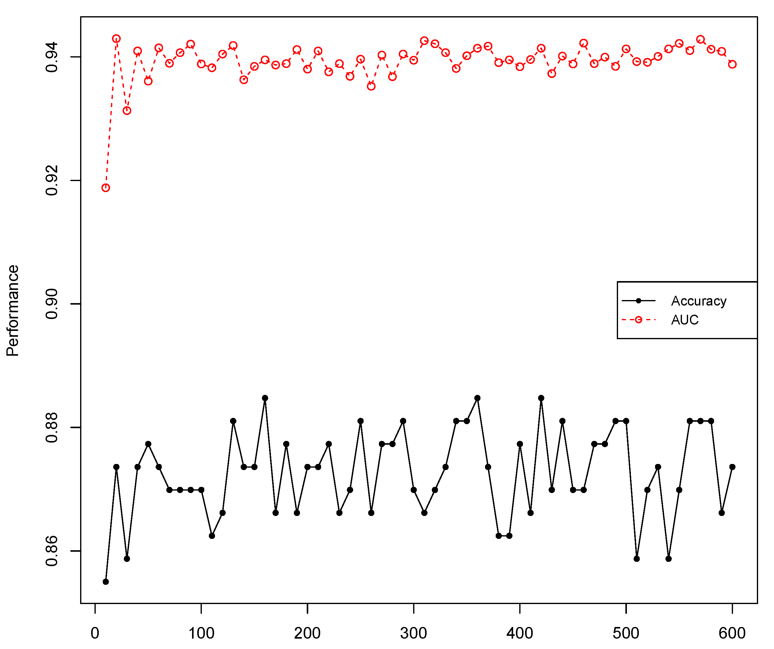
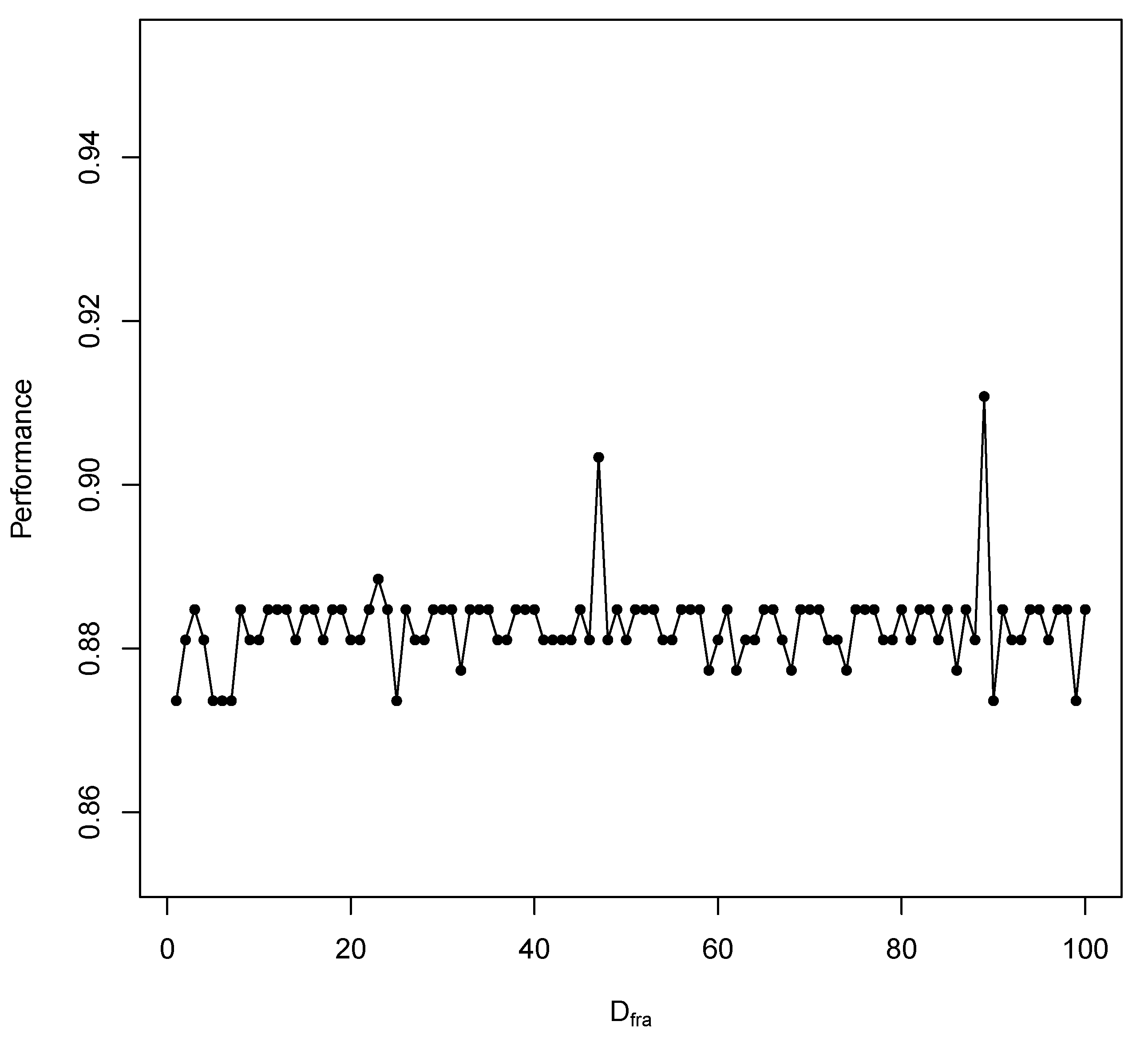
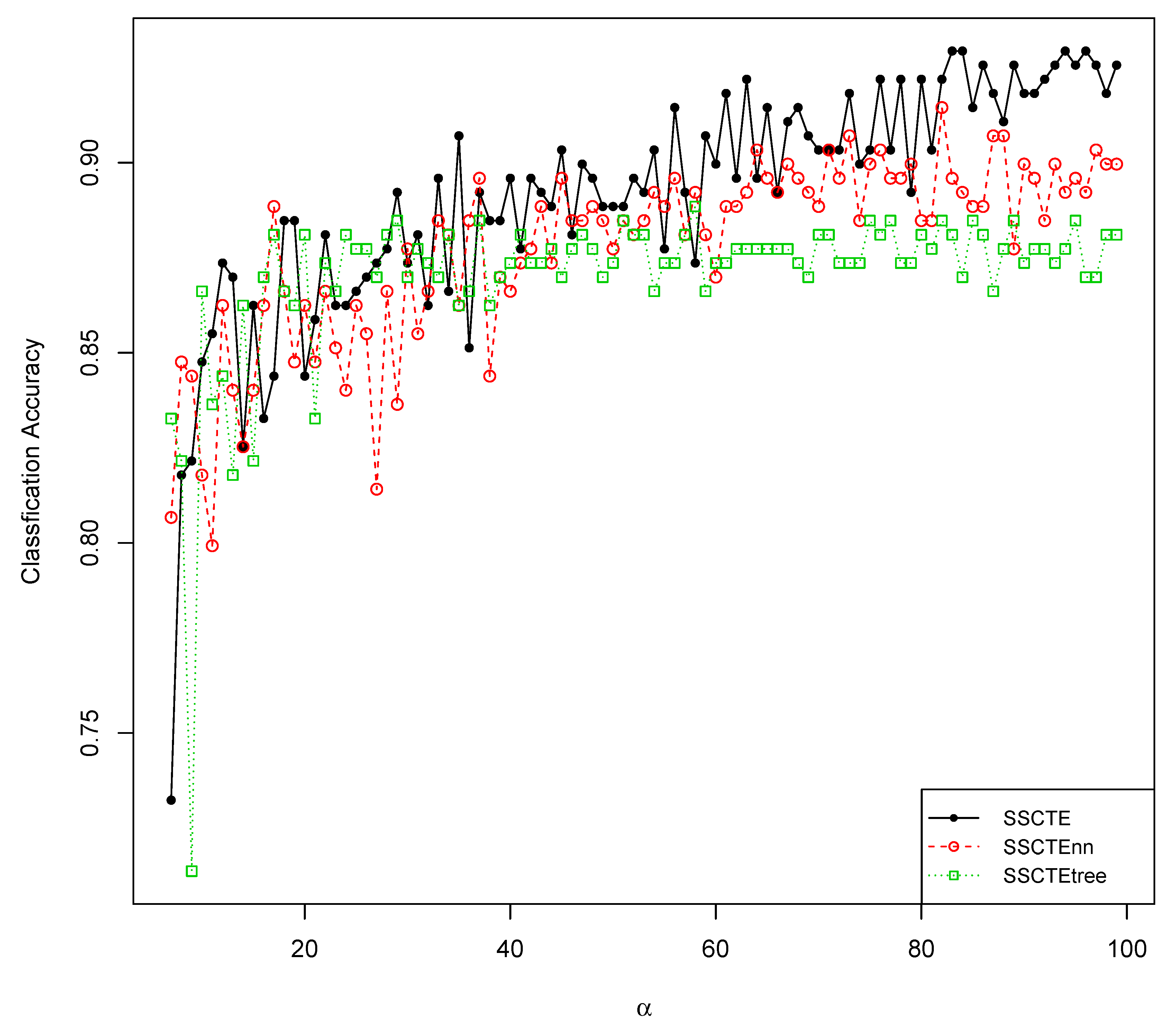
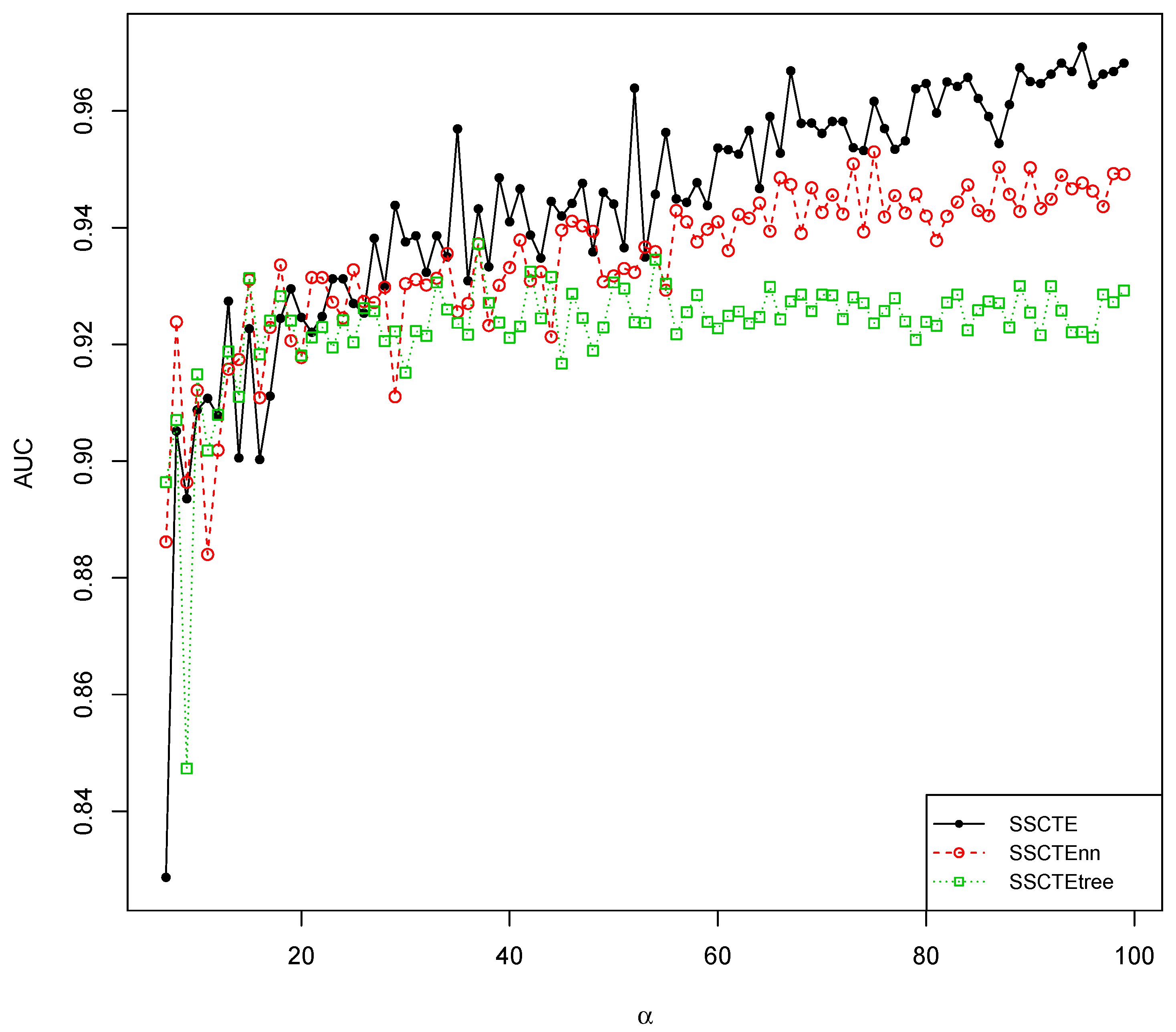
4.3.1. Parameter Sensitivity

First, we want to test the performance of SSCTE with different iterations k, where parameters D f r a and p c o n f use the algorithm default settings one and 0.95, respectively. As shown in Figure 4, SSCTE’s classification accuracy and AUC increase slowly when the number of iterations increases at the very beginning. This indicates that a larger ensemble size will lead to a relatively better performance. However, when k 40 , SSCTE is no longer too sensitive to the number of iterations. Thus, for efficiency and accuracy reasons, we choose k = 50 as the default setting in later experiments.
Next, we want to discover SSCTE’s performance using various amounts of diversity data, indicated by the D f r a factor. As shown in Figure 5, diversity data help to increase SSCTE’s performance when the amount of diversity data is small ( 1 D f r a 15 ) . However, when D f r a > 16 , SSCTE’s performance begins to deteriorate and becomes unstable. This is because the resulting training set contains too much noise data. For this reason, we recommend setting D f r a between 1–10 and in our later experiments; D f r a is set to one.
Figure 4. SSCTE’s performance with different iterations.
Information 05 00634 g004
Figure 5. SSCTE’s performance with various amount of diversity data.
Information 05 00634 g005

4.3.2. One versus Two
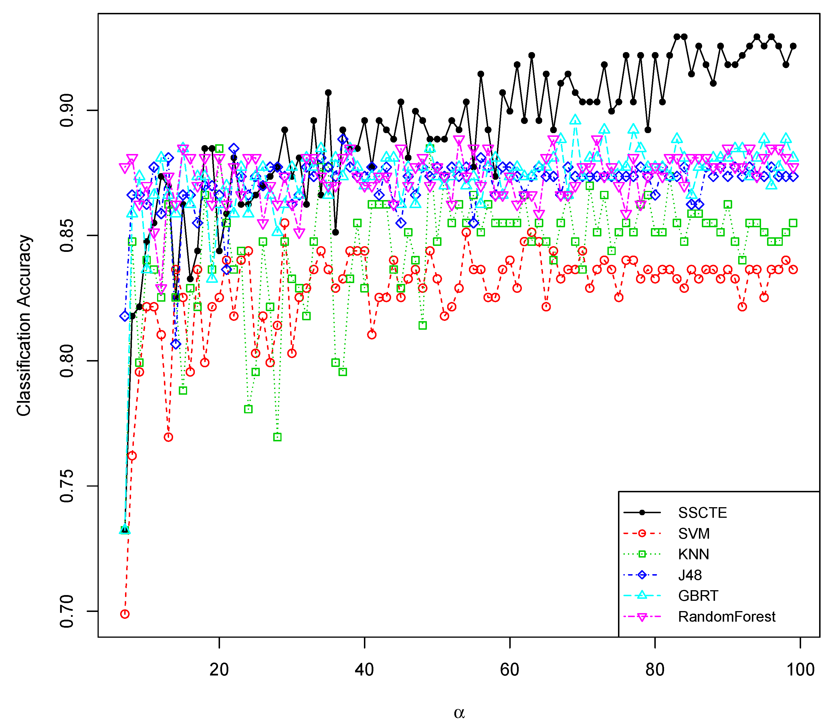
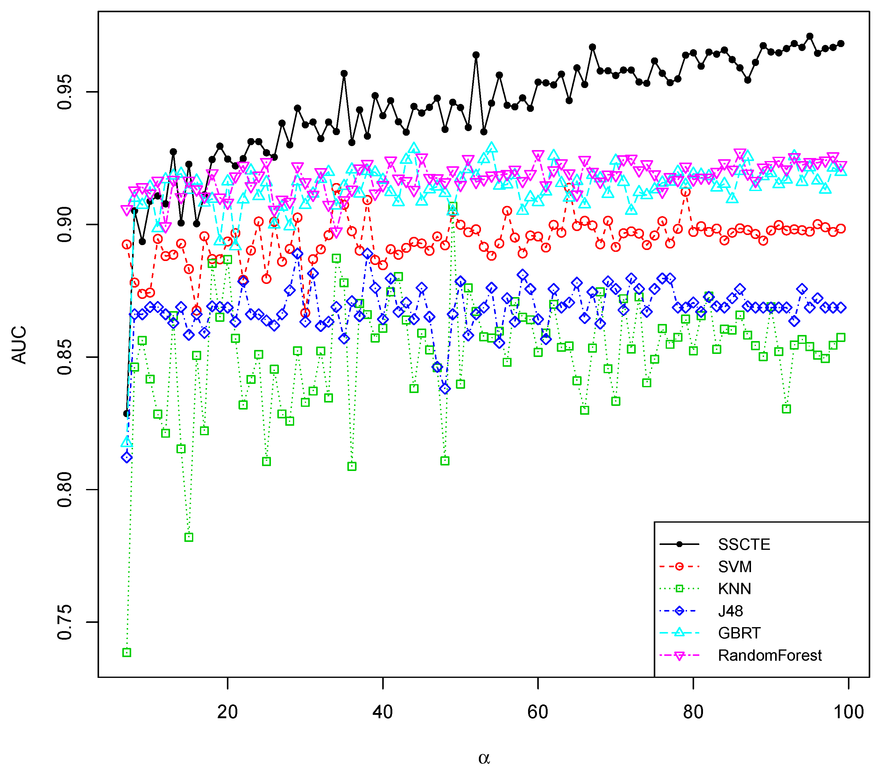
Here, we will test SSCTE’s performance under different combinations of base classifiers: SSCTE with neural networks and decision trees (SSCTE, the proposed algorithm), SSCTE with only neural networks (SSCTEnn) and SSCTE with only decision trees (SSCTEtree). For all of these three algorithms, the same settings, i.e., p c o n f = 0 . 95 , D f r a = 0 . 1 and k = 50 , are applied. In the experiments, unlabeled data are kept unchanged, and different sizes (controlled by α) of labeled examples are used as the labeled training set.
The results shown in Figure 6 and Figure 7 demonstrate that SSCTE beats the other two in most cases under both classification accuracy and AUC metrics. SSCTE is also much more stable than SSCEnn and SSCTEtree. This confirms our assumption that neural networks and decision trees are complementary to each other in the ensemble, and this combination of using two different kinds of base classifiers does improve the algorithm’s performance.
Figure 6. SSCTE variants’ performance in terms of classification accuracy (ACC).
Information 05 00634 g006
Figure 7. SSCTE variants’ performance in terms of AUC.
Information 05 00634 g007

4.3.3. Comparisons

Finally, we compare our SSCTE algorithm with state-of-the-art supervised learning algorithms: monolithic classifiers, such as SVM, KNN and J48 (Java C4.5); and ensemble classifiers, such as boosting (GBDT, gradient boosted decision trees) and random forests (RF).
The proposed SSCTE algorithm is implemented in R, a free software programming language for statistical computing. For SSCTE, we randomly choose α% ( α [ 7 , 99 ] ) of data from DMOZ-labeled training data and use it with DMOZ-unlabeled data to form a new training set. In SSCTE, p c o n f , D f r a and k are set to 0.95, 1 and 50, respectively. For supervised methods, only α% DMOZ-labeled data are used in training, and default parameters suggested in the R [41] packages are adopted. Hereafter, the reported performance of SSCTE and other methods corresponds to the result out of 93 runs on different percentages of the labeled training data, with unlabeled training data only for SSCTE.
Experimental results with different α in terms of classification accuracy and AUC are shown in Figure 8 and Figure 9, respectively.
As shown in Figure 8 and Figure 9, in terms of classification accuracy, SSCTE surpasses SVM, KNN, J48, GBDT and random forest in a majority of 98%, 97%, 80%, 81% and 81% cases and is inferior to these algorithms in 2%, 3%, 20%, 19% and 19% cases. In terms of AUC, SSCTE outperforms SVM, KNN, J48, GBDT and random forest in a majority, 99%, 100%, 100%, 94% and 92%, of cases, and is secondary to these models in much fewer, 1%, 0%, 0%, 6% and 8%, cases.
Figure 8. SSCTE’s performance in terms of ACC.
Information 05 00634 g008
Figure 9. SSCTE’s performance in terms of AUC.
Information 05 00634 g009
As expected, all approaches improve their results with the increase of α, i.e., the size of labeled data, especially at the very beginning. When α > 20 , most approaches, however, are not too sensitive to the size of the labeled data, while SSCTE still follows a relatively sharp increase in performance. This means that, if more labeled data are available, SSCTE always implies a better performance.
The Friedman rank sum test statistics for the above comparisons in terms of ACC and AUC are 319.853 and 425.725, respectively. This is significant (the corresponding p-value is less than 2 . 2 × 10 16 ), and a post hoc Nemenyi test was then applied to find out which pairs of algorithms are significantly different.
For the ease of notation, denote classifiers SSCTE, SVM, KNN, J48, GBRT and RF by A, B, C, D, E and F, respectively. The average ranks of classifiers A, B, C, D, E and F are:
R j A = 2 . 096774 , R j B = 4 . 623656 , R j C = 4 . 505376 R j D = 4 . 537634 , R j E = 3 . 021505 , R j F = 2 . 215054
Using the proposed algorithm (SSCTE, A) as the control algorithm and computing the z statistic of the Nemenyi test for different classifier pairs, we obtain:
z B A 1 = 9 . 2104 , z C A 1 = 8 . 7792 , z D A 1 = 8 . 8968 z E A 1 = 3 . 3706 , z F A 1 = 0 . 4311
Similarly, in the case of AUC metric, the corresponding z statistic values of the five classifier pairs are:
z B A 2 = 15 . 0110 , z C A 2 = 12 . 8553 , z D A 2 = 2 . 9787 z E A 2 = 8 . 8185 , z F A 2 = 6 . 5453
For α = 0 . 05 , the critical value of the studentized range distribution q α = 4 . 121 and divide q α value by 2 , we get the Nemenyi’s test critical value of 2.9140.
It can be seen that in terms of ACC, four Nemenyi statics z B A 1 , z C A 1 , z D A 1 , z E A 1 exceed 2.9140, while in terms of AUC, all five Nemenyi statics exceed the critical value. Thus, there exists significant differences between the proposed SSCTE and SVM, KNN, J48, GBRT in terms of ACC and also significant differences between SSCTE and SVM, KNN, J48, GBRT and random forests in terms of AUC. In other words, SSCTE is significantly better than SVM, KNN, J48 and GBRT under both the ACC and ACC metrics and is also significantly better than RF in terms of AUC.

5. Conclusions and Future Work

Determining whether an HTML web form is searchable or not is vital to further mining of the vast information of the Deep Web. Different from previous supervised approaches, we have adopted a semi-supervised co-training ensemble using neural networks and decision trees as the base classifiers.
In the proposed SSCTE algorithm, the bagging and random subspace method are exploited together to create a diverse ensemble. In SSCTE, data used to diversify the training set are generated from unlabeled data and, thus, extend the diversity data notion to a semi-supervised learning framework. Furthermore, the combination of neural networks and decision trees instead of using only one kind of base learners also increases the ensemble’s diversity.
Experimental results on the DMOZ datasets have shown that SSCTE outperforms state-of-the-art classifiers, such as SVM, KNN, random forests, boosting and C4.5 decision trees. In our ongoing work, we will work toward optimizing SSCTE’s parameters under different scenarios and seeking other base learners suitable for semi-supervised ensemble learning.

Acknowledgments

This work was supported in part by the National Natural Science Foundation of China (No.11271374 and No. 61003233). The authors want to thank Jinsong Lan and Youyang Chen for programming help in collecting the DMOZ dataset. The authors want to thank all of the reviewers for their valuable and constructive comments, which greatly improved the quality of this paper.

Author Contributions

This research was carried out in collaboration between all three authors. Hong Wang and Qingsong Xu defined the research theme. Hong Wang and Qingsong Xu designed the algorithm. Lifeng Zhou carried out the experiments and analyzed the data. Hong Wang and Lifeng Zhou interpreted the results and wrote the paper. All authors have read and approved the final manuscript.

Conflicts of Interest

The authors declare no conflict of interest.

References

  1. Bergman, M.K. White Paper: The deep web: Surfacing hidden value. J. Electron. Publ. 2001, 7. [Google Scholar] [CrossRef]
  2. Cope, J.; Craswell, N.; Hawking, D. Automated Discovery of Search Interfaces on the Web. In Proceedings of the 14th Australasian Database Conference (ADC2003), Adelaide, Australia, 4–7 February 2003; pp. 181–189.
  3. Madhavan, J.; Ko, D.; Kot, L.; Ganapathy, V.; Rasmussen, A.; Halevy, A. Google’s Deep Web crawl. Proc. VLDB Endow. 2008, 1, 1241–1252. [Google Scholar] [CrossRef]
  4. Khare, R.; An, Y.; Song, I.Y. Understanding deep web search interfaces: A survey. ACM SIGMOD Rec. 2010, 39, 33–40. [Google Scholar] [CrossRef]
  5. Hedley, Y.L.; Younas, M.; James, A.; Sanderson, M. Sampling, information extraction and summarisation of hidden web databases. Data Knowl. Eng. 2006, 59, 213–230. [Google Scholar] [CrossRef]
  6. Noor, U.; Rashid, Z.; Rauf, A. TODWEB: Training-Less ontology based deep web source classification. In Proceedings of the 13th International Conference on Information Integration and Web-based Applications and Services, Bali, Indonesia, 5–7 December 2011; ACM: New York, NY, USA, 2011; pp. 190–197. [Google Scholar]
  7. Balakrishnan, R.; Kambhampati, S. Factal: Integrating deep web based on trust and relevance. In Proceedings of the 20th international conference companion on World wide web, Hyderabad, India, 28 March–1 April 2011; ACM: New York, NY, USA, 2011; pp. 181–184. [Google Scholar]
  8. Palmieri Lage, J.; da Silva, A.; Golgher, P.; Laender, A. Automatic generation of agents for collecting hidden web pages for data extraction. Data Knowl. Eng. 2004, 49, 177–196. [Google Scholar] [CrossRef]
  9. Chang, K.; He, B.; Li, C.; Patel, M.; Zhang, Z. Structured databases on the web: Observations and implications. ACM SIGMOD Rec. 2004, 33, 61–70. [Google Scholar] [CrossRef]
  10. Ye, Y.; Li, H.; Deng, X.; Huang, J. Feature weighting random forest for detection of hidden web search interfaces. Comput. Linguist. Chin. Lang. Process. 2009, 13, 387–404. [Google Scholar]
  11. Barbosa, L.; Freire, J. Combining classifiers to identify online databases. In Proceedings of the 16th international conference on World Wide Web, Banff, AB, Canada, 8–12 May 2007; ACM: New York, NY, USA, 2007; pp. 431–440. [Google Scholar]
  12. Barbosa, L.; Freire, J. Searching for hidden-web databases. In Proceedings of the Eighth International Workshop on the Web and Databases (WebDB 2005), Baltimore, MD, USA, 16–17 June 2005; pp. 1–6.
  13. Shestakov, D. On building a search interface discovery system. In Proceedings of the 2nd International Conference on Resource Discovery, Lyon, France, 28 August 2009; pp. 81–93.
  14. Fang, W.; Cui, Z.M. Semi-Supervised Classification with Co-Training for Deep Web. Key Eng. Mater. 2010, 439, 183–188. [Google Scholar] [CrossRef]
  15. Chang, K.C.C.; He, B.; Zhang, Z. Metaquerier over the deep web: Shallow integration across holistic sources. In Proceedings of the 2004 VLDB Workshop on Information Integration on the Web, Toronto, Canada, 29 August 2004; pp. 15–21.
  16. Wang, Y.; Li, H.; Zuo, W.; He, F.; Wang, X.; Chen, K. Research on discovering deep web entries. Comput. Sci. Inf. Syst. 2011, 8, 779–799. [Google Scholar] [CrossRef]
  17. Marin-Castro, H.; Sosa-Sosa, V.; Martinez-Trinidad, J.; Lopez-Arevalo, I. Automatic discovery of Web Query Interfaces using machine learning techniques. J. Intell. Inf. Syst. 2013, 40, 85–108. [Google Scholar] [CrossRef]
  18. Bergholz, A.; Childlovskii, B. Crawling for domain-specific hidden Web resources. In Proceedings of the Fourth International Conference on Web Information Systems Engineering, WISE 2003, Roma, Italy, 10–12 December 2003; pp. 125–133.
  19. Lin, L.; Zhou, L. Web database schema identification through simple query interface. In Proceedings of the 2nd International Conference on Resource Discovery, Lyon, France, 28 August 2009; pp. 18–34.
  20. Chapelle, O.; Schölkopf, B.; Zien, A. Semi-Supervised Learning; MIT press: Cambridge, MA, USA, 2006. [Google Scholar]
  21. Zhu, X. Semi-Supervised Learning Literature Survey. Available online: http://pages.cs.wisc.edu/jerryzhu/research/ssl/semireview.html (accessed on 28 November 2014).
  22. Roli, F. Semi-supervised multiple classifier systems: Background and research directions. Mult. Classif. Syst. 2005, 3541, 674–676. [Google Scholar]
  23. Zhou, Z.; Li, M. Semi-supervised learning by disagreement. Knowl. Inf. Syst. 2010, 24, 415–439. [Google Scholar] [CrossRef]
  24. Polikar, R. Ensemble based systems in decision making. IEEE Circuits Syst. Mag. 2006, 6, 21–45. [Google Scholar] [CrossRef]
  25. Zhou, Z. When semi-supervised learning meets ensemble learning. Mult. Classif. Syst. 2009, 5519, 529–538. [Google Scholar]
  26. Breiman, L. Bagging predictors. Mach. Learn. 1996, 24, 123–140. [Google Scholar] [CrossRef]
  27. Freund, Y.; Schapire, R.E. A decision-theoretic generalization of on-line learning and an application to boosting. J. Comput. Syst. Sci. 1997, 55, 119–139. [Google Scholar] [CrossRef]
  28. Ho, T.K. The random subspace method for constructing decision forests. IEEE Trans. Pattern Anal. Mach. Intell. 1998, 20, 832–844. [Google Scholar]
  29. d’Alchè, F.; Grandvalet, Y.; Ambroise, C. Semi-supervised marginboos. In Advances in Neural Information Processing Systems 14; MIT Press: Cambridge, MA, USA, 2002; pp. 553–560. [Google Scholar]
  30. Freund, Y.; Schapire, R.E. Experiments with a new boosting algorithm. ICML 1996, 96, 148–156. [Google Scholar]
  31. Bennett, K.; Demiriz, A.; Maclin, R. Exploiting unlabeled data in ensemble methods. In Proceedings of the eighth ACM SIGKDD international conference on knowledge discovery and data mining, Edmonton, AB, Canada, 23–25 July 2002; ACM: New York, NY, USA, 2002; pp. 289–296. [Google Scholar]
  32. Mallapragada, P.; Jin, R.; Jain, A.; Liu, Y. SemiBoost: Boosting for Semi-Supervised Learning. IEEE Trans. Pattern Anal. Mach. Intell. 2009, 31, 2000–2014. [Google Scholar] [CrossRef] [PubMed]
  33. Li, M.; Zhou, Z.H. Improve Computer-Aided Diagnosis With Machine Learning Techniques Using Undiagnosed Samples. IEEE Trans. Syst. Man Cybern. 2007, 37, 1088–1098. [Google Scholar] [CrossRef]
  34. Melville, P.; Mooney, R.J. Constructing diverse classifier ensembles using artificial training examples. In Proceedings of the 18th International Joint Conference on Artificial Intelligence, Acapulco, Mexico, 9–15 August 2003; pp. 505–510.
  35. Breiman, L. Random forests. Mach. Learn. 2001, 45, 5–32. [Google Scholar] [CrossRef]
  36. Friedman, J.H. Stochastic gradient boosting. Comput. Stat. Data Anal. 2002, 38, 367–378. [Google Scholar] [CrossRef]
  37. Liu, Y.; Yao, X. Ensemble learning via negative correlation. Neural Netw. 1999, 12, 1399–1404. [Google Scholar] [CrossRef]
  38. Blum, A.; Mitchell, T. Combining labeled and unlabeled data with co-training. In Proceedings of the Eleventh Annual Conference on Computational Learning Theory, Madison, WI, USA, 24–26 July 1998; ACM: New York, NY, USA, 1998; pp. 92–100. [Google Scholar]
  39. Fawcett, T. An introduction to ROC analysis. Pattern Recogn. Lett. 2006, 27, 861–874. [Google Scholar] [CrossRef]
  40. Demšar, J. Statistical comparisons of classifiers over multiple data sets. J. Mach. Learn. Res. 2006, 7, 1–30. [Google Scholar]
  41. R Core Team. R: A Language and Environment for Statistical Computing; R Foundation for Statistical Computing: Vienna, Austria, 2012; ISBN 3-900051-07-0. [Google Scholar]

