Abstract
The accuracy of reservoir flow forecasting has the most significant influence on the assurance of stability and annual operations of hydro-constructions. For instance, accurate forecasting on the ebb and flow of Vietnam’s Hoabinh Reservoir can aid in the preparation and prevention of lowland flooding and drought, as well as regulating electric energy. This raises the need to propose a model that accurately forecasts the incoming flow of the Hoabinh Reservoir. In this study, a solution to this problem based on neural network with the Cuckoo Search (CS) algorithm is presented. In particular, we used hydrographic data and predicted total incoming flows of the Hoabinh Reservoir over a period of 10 days. The Cuckoo Search algorithm was utilized to train the feedforward neural network (FNN) for prediction. The algorithm optimized the weights between layers and biases of the neuron network. Different forecasting models for the three scenarios were developed. The constructed models have shown high forecasting performance based on the performance indices calculated. These results were also compared with those obtained from the neural networks trained by the particle swarm optimization (PSO) and back-propagation (BP), indicating that the proposed approach performed more effectively. Based on the experimental results, the scenario using the rainfall and the flow as input yielded the highest forecasting accuracy when compared with other scenarios. The performance criteria RMSE, MAPE, and R obtained by the CS-FNN in this scenario were calculated as 48.7161, 0.067268 and 0.8965, respectively. These results were highly correlated to actual values. It is expected that this work may be useful for hydrographic forecasting.
1. Introduction
The prediction of hydrographic factors, especially flow forecasting, plays an important role in water resource reconcilement as well as in the prevention of natural calamities. A reservoir is one of the defense mechanisms for flood and drought disasters. During the flood period, the opening of the dam’s spillway gate should be adequate to ensure that the reservoir capacity will not exceed its limits and the discharges will not cause overflow downstream; during the drought period, the reservoir needs to impound water and release adequately to fulfill water demands. Such operations require a model capable of accurately forecasting incoming flow. The flow forecasts of water reservoirs as one of the hydrographic forecast study fields has been developed to meet essential water reconcilement procedures, hydroelectric problems, and agricultural irrigations. Since high forecasting accuracy can significantly reduce the economic losses of the state and its people, this field of study has gained much attention.
Intelligent approaches have been used to tackle different science and engineering problems. The artificial neural network (ANN) was determined to be a successful tool to predict the interfacial tension at the crystal/solution interface [1]. Chamkalani et al. [2] showed the superiority of the least square support vector machine in predicting the compressibility factor in the petroleum industry. ANN optimized with Particle Swarm Optimization algorithm was found to be the best model in predicting Recovery Factor and Cumulative Steam to Oil Ration during steamflooding [3]. It was also proven that ANN is an efficient tool for the prediction of pure organic compounds’ surface tensions for a wide range of temperatures [4]. An ANN model, optimized by the imperialist competitive algorithm, was efficiently applied to predicting the amount of asphaltene precipitation and bubble point pressure for a conventional oil sample during successive depressurization stages [5]. Among intelligent approaches, ANN, a soft computing technique, has emerged as one of the most powerful tools in many disciplines [6,7,8,9,10,11,12]. Artificial neural networks have the notable ability to derive meaning from complicated or imprecise data, and can be used to extract patterns and detect trends that are too complicated to be recognized by either humans or computing techniques. These are appropriate for continuous valued inputs and outputs. Neural networks are best at identifying patterns or trends in data and well suited for prediction and forecasting needs.
When a neural network is structured for a particular application, it must be trained before being used to classify testing data. The aim of the training phase is to minimize a cost function defined as the mean squared error or sum of squared error between its actual and target outputs by adjusting weights and biases. Presenting a satisfactory and efficient training algorithm has always been a challenging subject. A popular approach used in the training phase is the back-propagation (BP) algorithm which includes the standard BP [13] and the improved BP [14,15,16]. However, researchers have pointed out that the BP algorithm—a gradient-based algorithm—has disadvantages [17,18,19]. Heuristic algorithms are known for their ability to produce optimal or near optimal solutions for optimization problems. Cuckoo Search (CS) is a recent heuristic algorithm proposed by Yang and Deb [20,21]. Among the heuristic algorithms, the CS is considered as one of the most powerful ones. When given enough computation, the CS will always find the optimal solution. The CS and improved CS algorithms have been used in solving various problems, and is considered to outperform other algorithms [21,22,23,24]. Therefore, in this study, we used CS in training neural networks.
There are a number of factors that can affect flow forecasts, such as: rainfall, temperature, humidity, soil, geological elements, and human activities. However, in this work, the slow-varying factors can be omitted as inputs for the calculation because they have only a small effect. Of the main weather related factors, rainfall is the most influential factor. Equally influential to flow forecasting is how much water the reservoir can naturally hold. Regarding the period of the prediction, forecast methods can be categorized into several models: short term forecast (1–2 days ahead); mid-term forecast (5–10 days ahead); long term forecast (1 month ahead); and, ultra long term forecast (for a season). In this study, we solve the problem of forecasting total incoming flows of the Hoabinh Reservoir over a period of the next 10 days. Our proposed models have been constructed with some essential input factors, which are refined and optimized for efficiency. Finally, the outputs are compared to retrieve the best model for flow forecasting.
The paper is organized into six sections: an introduction in Section 1, the literature review is provided in Section 2; the CS algorithm is presented in Section 3; Section 4 is dedicated to describing the process of neural network training, the research design is provided in Section 5; results are shown in Section 6; and finally, Section 7 presents the conclusion.
2. Literature Review
The ANN has been widely used in different applications. This section provides a glimpse into the literature concerning the use of ANN in water modeling and water resources management. Dolling and Varas [8] developed neural networks to predict flows during the spring and summer season for San Joan River basin, Argentina. They used meteorological information gathered during April, May and June as input variables. Output variables were the seven monthly flows for the period of July through January. The results showed that a feed-forward neural network having an architecture 30-20-7 had a good performance. Ünes [25] used an ANN, a two-dimensional mathematical model, and a multiple linear regression (MLR) model to investigate the plunging flow parameters. A one-hidden layer multilayer perceptron (MLP) with four nodes and one output neuron was used as the ANN structure. In order to evaluate the performances of different models, the criteria, including mean square error, mean absolute error, and correlation coefficient were used. The results indicated that the ANN model forecasts are much closer to the experimental data than the MLR and mathematical model forecasts. Sivapragasam et al. [12] used the multilayer feedforward network (FNN) with back-propagation learning algorithm to forecast monthly flows of the Mississipi River at the Vicksburg gauging station. This study concluded that it is better to develop individual models for each month separately with information from previous years for the same month. Akhtar et al. [26] used ANN to predict the river flow at the Hardinge Bridge (Bangladesh). Their model was based on the ANN multi-layer perceptron networks trained with gradient based methods. The ANN showed its ability to forecast discharges 3 days ahead with an acceptable accuracy. The study found that one-day previous discharge along with composite rainfall gives the best results in comparison with other options. Taghi Sattaria et al. [27] evaluated the performances of different neural networks in predicting of daily reservoir inflow to the Eleviyan reservoir in Iran. In the study, the daily inflow into the Eleviyan reservoir between the years 2004–2007 was considered. The obtained results showed that performance statistics of 8-1-1 (8 inputs, 1 hidden layer, and 1 output layer) MLP architecture was best in predicting the inflow in this dataset. An ANN model was developed to forecast river flow in the Apalachicola River [28]. The model used a feed-forward, back-propagation network structure with an optimized conjugated training algorithm. This study used long-term observations of rainfall and river flow during 1939–2000 [28]. The results indicated that the neural network model developed in this study was capable of providing good forecasting of river flow at different time-scales. Results obtained from the ANN model were also compared with those from a traditional autoregressive integrated moving average (ARIMA) forecasting model. Results showed that the ANN model provided better accuracy in forecasting river flow than did the ARIMA model.
The above mentioned studies revealed that ANN-based models have been successfully used in the area of river flow forecasting. However, in order to increase the reliability of forecasting results of the ANN-based model, there is a need to focus attention on optimizing the parameters of the model. In other words, training phase plays an important role in developing the ANN-based models. In the examined literature, the BP algorithm, a gradient-based algorithm, has been widely used in the training phase. However, many studies have pointed out the drawbacks of this algorithm, including the tendency to become trapped in local minima [29] and having a slow convergence [30]. Heuristic algorithms, including genetic algorithm (GA) [31], particle swarm optimization (PSO) [32], and ant colony optimization (ACO) [33], have also been proposed for the purpose of training. Recently, several heuristic algorithms inspired by the behavior of natural phenomena were developed for solving optimization problems and have been proven to be effective. The Cuckoo Search (CS), proposed by Yang and Deb [20], was inspired by the egg laying and breeding characteristics of the Cuckoo birds. Studies have shown that CS outperformed other algorithms such as PSO and GA [22,23,24]. Moreover, the CS is capable of reducing the aforementioned drawbacks of back propagation.
Taking into account the available literature, there is still room for the improvement of the ANN-based models in the problem of flow forecasting. This leads us to propose a new approach in this study for accomplishing a successful forecasting of incoming flows. The merit of the CS algorithm and the success of ANN in the prediction and forecasting have encouraged us to combine ANN and the CS algorithm. In this study, we propose an approach based on the multilayer feed-forward network improved by the CS algorithm for forecasting incoming flows, which makes use of the optimizing ability of the CS algorithm. In general, the scientific contribution provided by the current research is the new approach applied herein. To the best of our knowledge, this combination of the two artificial intelligence techniques is applied for the first time in the forecasting field. Although the models are developed for a specific application, they can be used as basic guides for other application areas.
3. Cuckoo Search Algorithm
The CS was inspired by the special lifestyle of the cuckoo species [20,21]. The cuckoo birds lay their eggs in the nests of host birds and they may remove the eggs of the host bird. In the process, some of these eggs, which look similar to the host bird’s eggs, have the opportunity to grow up and become adult cuckoos. In other cases, the eggs are discovered by host birds and the host birds will throw them away or leave their nests and find other places to build new ones. Each egg in a nest represents a solution, and a cuckoo egg stands for a new solution. The CS uses new and potentially better solutions to replace inadequate solutions in the nests. The CS is based on the following rules: each cuckoo lays one egg at a time, and dumps this egg in a randomly chosen nest; the best nests with high quality eggs (solutions) will carry over to the next generation; and the number of available host nests is fixed, and a host bird can detect an alien egg with a probability of pa ∊ [0,1]. In this case, the host bird may either throw the egg away or abandon the nest to build a new one in a new place. The last assumption can be estimated by the fraction pa of the n nests being replaced by new nests (with new random solutions). For a maximization problem, the quality or fitness of a solution can be proportional to the objective function. Other forms of fitness can be defined in a similar way to the fitness function in genetic algorithms. Based on the above mentioned rules, the steps of the CS can be described as the pseudo code as shown Algorithm 1. The algorithm can be extended when each nest has multiple eggs representing a set of solutions.
| Algorithm 1. Pseudo code of the Cuckoo Search (CS). |
| Begin |
| Objective function f(x), x= (x1,...,xd)T |
| Generate an initial population of n host nests xi (i=1,2,...,n), each nest containing a random solution; |
| while (t <MaxGeneration) or (stop criterion); |
| Get a cuckoo randomly by Lévy flights; |
| Evaluate its quality/fitness Fi; |
| Choose a nest among n (say, j) randomly; |
| if (Fi > Fj), |
| Replace j by the new solution; |
| end |
| A fraction (pa) of worse nests are replaced by new random solutions via Lévy flights; |
| Keep the best solutions (or nests with quality solutions); |
| Rank the solutions and find the current best; |
| Pass the current best solutions to the next generation; |
| end while |
| Return the best nest; |
| End |
When generating new solutions, x(t+1), for the ith cuckoo at iteration (t+1), the following Lévy flight is performed:
 where α > 0 is the step size, which depends on the scale of the problem. The product
  denotes entry-wise multiplications. Lévy flights provide a random walk. The Lévy flight is a probability distribution which has an infinite variance with an infinite mean. It is represented by:
There are several ways to achieve random numbers in Lévy flights; however, a Mantegna algorithm is the most efficient [21]. In this work, the Mantegna algorithm was utilized to calculate this step length.
denotes entry-wise multiplications. Lévy flights provide a random walk. The Lévy flight is a probability distribution which has an infinite variance with an infinite mean. It is represented by:
Lévy ~ u = t−λ, (1<λ≤3)
Studies have indicated that CS is very efficient in dealing with optimization problems. However, several recent studies made some improvements to make the CS more practical for a wider range of applications without losing the advantages of the standard CS [34,35,36]. Notably, Walton et al. [37] made two modifications to increase the convergence rate of the CS. The first modification was made to the size of the step size α. In the standard CS, α is constant; whereas, in the modified CS, α decreases when the number of generations increases. The second modification was to add an information exchange between the eggs to speed up convergence to a minimum. In the standard CS, the searches are performed independently and there is no information exchange between individuals. However, in the modified CS, there is a fraction of eggs with the best fitness that are put into a group of top eggs. It has also been indicated that adding the random biased walk to modified CS results in an efficient optimization algorithm [38]. However, in this work, we use the standard CS for training neural networks to forecast incoming flow.
4. Training Artificial Neural Network
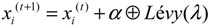
An ANN has two types of basic components, namely, neuron and link. A neuron is a processing element and a link is used to connect one neuron with another. Each link has its own weight. Each neuron receives stimulation from other neurons, processes the information, and produces an output. Neurons are organized into a sequence of layers. The first and the last layers are called input and output layers, respectively, and the middle layers are called hidden layers. The input layer is a buffer that presents data to the network. It is not a neural computing layer because it has no input weights and no activation functions. The hidden layer has no connections to the outside world. The output layer presents the output response to a given input. The activation coming into a neuron from other neurons is multiplied by the weights on the links over which it spreads, and is then added together with other incoming activations. A neural network in which activations spread only in a forward direction from the input layer through one or more hidden layers to the output layer is known as a multilayer feedforward neural network (FNN). For a given set of data, a multi-layer FNN can provide a good non-linear relationship. Studies have shown that an FNN even with only one hidden layer can approximate any continuous function [39]. Therefore, an FNN is an attractive approach [40]. Figure 1 shows an example of an FNN with one hidden layer. In Figure 1, R, N, and S are the numbers of input, hidden neurons, and output, respectively; iw and hw are the input and hidden weights matrices, respectively; hb and ob are the bias vectors of the hidden and output layers, respectively; x is the input vector of the network; ho is the output vector of the hidden layer; and y is the output vector of the network. The neural network in Figure 1 can be expressed through the following equations:
 where f is an activation function.
When implementing a neural network, it is necessary to determine the structure in terms of number of layers and number of neurons in the layers. The larger the number of hidden layers and nodes, the more complex the network will be. A network with a structure that is more complicated than necessary over fits the training dataset [41]. This means that it performs well on data included in the training dataset, but may perform poorly on that in a testing dataset.
Figure 1.
A feedforward neural network (FNN) with one hidden layer.
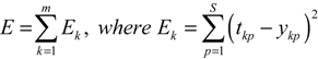
Once a network has been structured for a particular application, it is ready for training. Training a network means finding a set of weights and biases that will give desired values at the network’s output when presented with different patterns at its input. When network training is initiated, the iterative process of presenting the training dataset to the network’s input continues until a given termination condition is satisfied. This usually happens based on a criterion indicating that the current achieved solution is good enough to stop training. Some of the common termination criteria are sum of squared error (SSE) and mean squared error (MSE). Through continuous iterations, the optimal solution is finally achieved, which is regarded as the weights and biases of a neural network. Suppose that there are m input-target sets, xkp−tkp for k = 1, 2,..., m and p = 1,2,...,S; ykp and tkp are predicted and target values of pth output unit for sample k. Thus, network variables arranged as iw, hw, hb, and ob are to be changed to minimize an error function, E, such as the SSE between network outputs and desired targets is as follows:
5. Research Design
The forecasting model development includes: (1) collecting the dataset, (2) selecting an ANN structure, (3) selecting transfer functions, (4) selecting a training algorithm, and (5) evaluating the model performance. In this section, the process of developing a forecasting model based on ANN and CS is represented.
5.1. Scenarios
Three different scenarios were developed to forecast flow. In all scenarios, different combinations of inputs were taken into account. The output of the forecasting models in all scenarios was the predicted flow Q(t+10), indicating the water flow that will occur over the next 10 days. The details of each scenario are given in the following paragraphs.
The first scenario: Suppose Q(t) is the flow at the current time. In this scenario, the inputs are: the current flow Q(t), the flow over the last 10 days Q(t−10), and the flow over the last 20 days Q(t−20).
The second scenario: For the hydrographic study, the rainfall on the rivers’ valleys is also directly influenced by the incoming flows that appear in the front of dedicated water reservoirs. Therefore, in this scenario, we considered the rainfall in the relative times of measurements as inputs. Suppose X(t) is the current rainfall. The inputs include: the current flow Q(t), the flow over the last 10 days Q(t−10), the flow over the last 20 days Q(t−20), the rainfall amount at the current time X(t), the rainfall amount over the last 10 days X(t−10), and the rainfall amount over the last 20 days X(t−20).
The third scenario: In this scenario, we consider the rainfall and the flow measured over the current entire day as inputs. Hence, there are eight inputs: the current flow Q(t); the flow over the last 10 days Q(t−10), the flow over the last 20 days Q(t−20), the rainfall amount of the current time X(t), the rainfall amount over the last 10 days X(t−10), the rainfall amount over the last 20 days X(t−20), the rainfall measured over the current entire day Xday(t), and the flow measured over the current entire day Qday(t).
The flow is measured in cubic meters per second (m3/s) and the unit for rainfall measurement is millimeters (mm).
5.2. Dataset
The dataset was retrieved from hydrographic data in the years of 1990–2012 at the Tabu gauging station by the Songda River (the closest station that faces the front of the Hoabinh Reservoir). The measurements were taken in the dry season (from December to May of the following year). The dataset was divided into two groups. The first group (68% of the dataset) (from the end of 1990 to the beginning of 2005) was used for training the model. The second group (32% of the dataset) (from the end of 2005 to the beginning of 2012) was employed for testing the model. The training dataset served in model building, while the testing dataset was used for validating the developed model.
5.3. Structure of the Neural Network
The structure of an ANN is dictated by the choice of the number in the input, hidden, and output layers. Each dataset has its own particular structure, and therefore determines the specific ANN structure. The number of neurons comprised in the input layer is equal to the number of features (input variables) in the data. The number of neurons in the output layer is equal to the number of output variables. The three layer FNN was utilized in this work since it can be used to approximate any continuous function [42,43]. Regarding the number of hidden neurons, the choice of an optimal size of hidden layer has often been studied, but a rigorous generalized method has not been found [44]. Hence, the trial-and-error method is the most commonly used method for estimating the optimum number of neurons in the hidden layer. In this method, various network architectures are tested in order to find the optimum number of hidden neurons [45]. In this study, the choice was also made through extensive simulation with different choices of the number of hidden nodes. For each choice, we obtained the performance of the concerned neural networks, and the number of hidden nodes providing the best performance was used for presenting results. The activation function from input to hidden is sigmoid. With no loss of generality, a commonly used form, f(n) = 2/(1 + e−2n) − 1, is utilized; while a linear function is used from the hidden to output layer.
5.4. Encoding Strategy
There are three ways of encoding and representing the weights and biases of FNN for every solution in evolutionary algorithms [30]. They are the vector, matrix, and binary encoding methods. In this study, we utilized the vector encoding method. The objective function is to minimize error values. The CS algorithm was used to search optimal weights and biases of neural networks. The amount of error is determined by the squared difference between the target output and actual output. In the implementation of the CS algorithm to train a neural network (CS-FNN), all training parameters, θ = {iw, hw, hb, ob}, are converted into a single vector of real numbers, as shown in Figure 2. Each vector represents a complete set of FNN weights and biases.
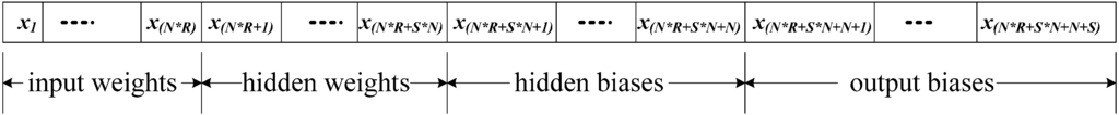
Figure 2.
The vector of training parameters.
The aim of the training phase is to identify the optimal or near-optimal parameter, θ*, from the cost function E(θ).
5.5. Examining the Performance
To examine the performance of a neural network, several criteria are used. These criteria are applied to the trained neural network to determine how well the network works. These criteria are used to compare predicted values and actual values. They are as follows:
Root mean squared error (RMSE): This index estimates the residual between the actual value and predicted value. A model has better performance if it has smaller a RMSE. An RMSE equal to zero represents a perfect fit.
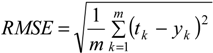 where tk is the actual value, yk is the predicted value produced by the model, and m is the total number of observations.
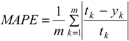
Mean absolute percentage error (MAPE): This index indicates an average of the absolute percentage errors; the lower the MAPE the better.
 Correlation coefficient (R): This criterion reveals the strength of relationships between actual values and predicted values. The correlation coefficient has a range from 0–1, and a model with a higher R means it has better performance.
 where
where  and
and  are the average values of tk and yk, respectively.
and are the average values of tk and yk, respectively.6. Experimental Results
In the following experiments, we used the CS algorithm to train FNN (CS-FNN) for flow forecasting in three mentioned scenarios. The model were coded and implemented in the MATLAB environment (MATLAB R2014a) [46]. A five-fold cross validation method was utilized to avoid over-fitting. As mentioned, the one-hidden-layer network architecture was used. The optimum number of neurons in the hidden layer was determined by varying their number, starting with a minimum of one and then increasing in steps by adding one neuron each time. In other words, various network architectures were tested in order to obtain the best performing architecture. The best performing ANN architecture for the dataset used was then identified, thus, providing the results with the smallest error values during the training. Initially, weights and biases were set in the range of [−10, 10]. Different parameters were tried to obtain the best performance. The parameters for CS were set as follows: the step size (α) was 0.01; the number of nests was 30; the net discovery rate (pa) was 0.1.
To show the efficiency of the proposed approach, the FNNs using PSO (PSO-FNN) and BP (BP-FNN) for training were also applied to the problem. Different parameters were tried to obtain the best performance. For BP-FNN, the gradient descent with momentum (GDM) method was used; with a learning rate µ of 0.01 and a momentum α of 0.9. For PSO-FNN, the number of initial population was 30 with c1 and c2 set to 2, w decreased linearly from 0.9–0.4, and the initial velocities of particles were randomly generated in [0,1]. The criterion for finishing the training process was the completion of the maximum number of iterations (equal to 500 in this study).
In the first scenario, the dataset included three input variables and one output variable. For the first scenario, the best performing architecture was 3-4-1, that is, with one hidden layer and four neurons, which resulted in a total of 16 weights and five biases. Table 1 showed the performance comparisons on the testing dataset for the three algorithms. The forecasting values and actual values were presented in Figure 3. In the figure, the data index (testing sample no.) is on x-axis and the values of the incoming flow along the y-axis. The differences between the actual and forecasting values of the incoming flow are called errors. There will always be errors of forecasting. By sight, we can know whether the model performs well.

Table 1.
Performance statistics of the models on testing dataset in the first scenario.
| Model | RMSE | MAPE | R |
|---|---|---|---|
| BP-FNN | 110.49 | 0.157268 | 0.7509 |
| CS-FNN | 99.2994 | 0.135368 | 0.7762 |
| PSO-FNN | 101.0622 | 0.136568 | 0.772 |
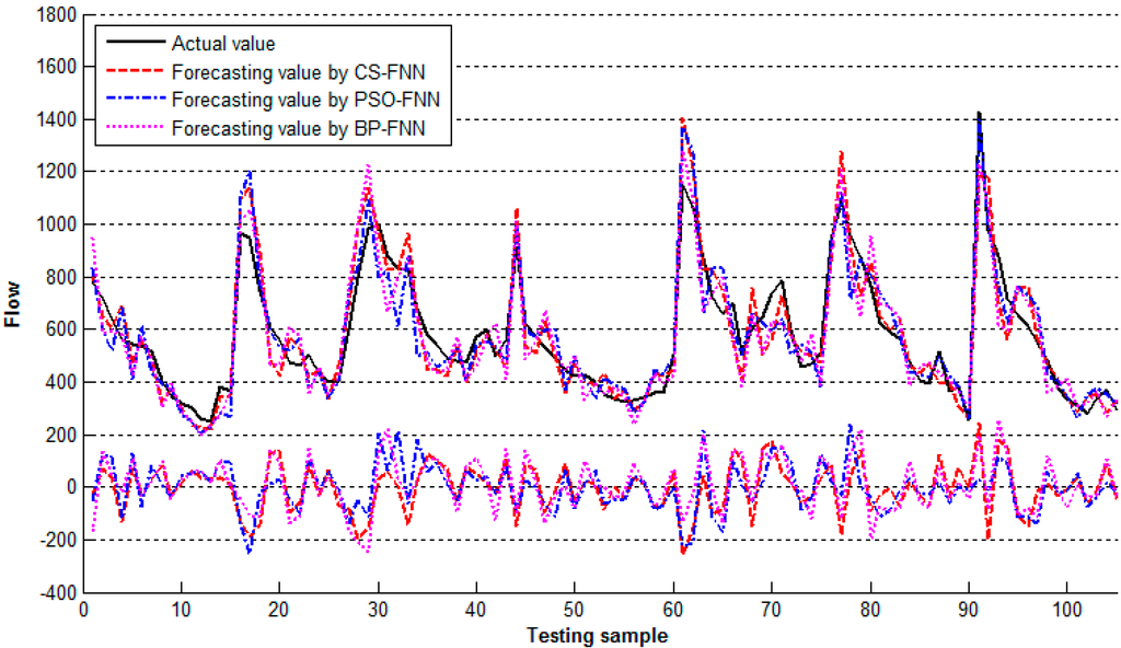
Figure 3.
The forecasting and actual values in the first scenario.
In the second scenario, the dataset included six input variables and one output variable. For this scenario, the best performing architecture was 6-8-1, that is, with one hidden layer and eight neurons, which resulted in a total of 56 weights and nine biases. Table 2 presented the performance comparisons on the testing dataset for the three algorithms. The forecasting values and actual values were presented in Figure 4.
In the third scenario, the dataset included eight input variables and one output variable. For the third scenario, the best performing architecture was 8-9-1, that is, with one hidden layer and nine neurons, which resulted in a total of 81 weights and 10 biases. Table 3 presented the performance comparisons on the testing dataset for the three algorithms. The forecasting values and actual values were presented in Figure 5. To analyze the quality of forecasting, the percentage of accurate forecasts (PAF) of the forecasting model was additionally investigated on the testing dataset. The PAF among all forecasts was calculated as the number of accurate forecasts divided by the total number of forecasts. In our study, an accurate forecast was defined as the forecast in which the forecasting value is within 90%–110% of the actual value (i.e., the forecasting error is ±10%). The higher the PAF, the more effective the model. For the third scenario, the PAF results indicated that the proposed CS-FNN model can reach a PAF value of 86.67%, whereas the PSO-FNN and BP-FNN models reach 58.09% and 49.52%, respectively. This means that the proposed CS-FNN model yielded the highest PAF.
Table 2.
Performance statistics of the models on testing dataset in the second scenario.
| Model | RMSE | MAPE | R |
|---|---|---|---|
| BP-FNN | 103.22 | 0.142246 | 0.7866 |
| CS-FNN | 84.0647 | 0.116846 | 0.8179 |
| PSO-FNN | 100.5382 | 0.131646 | 0.7964 |
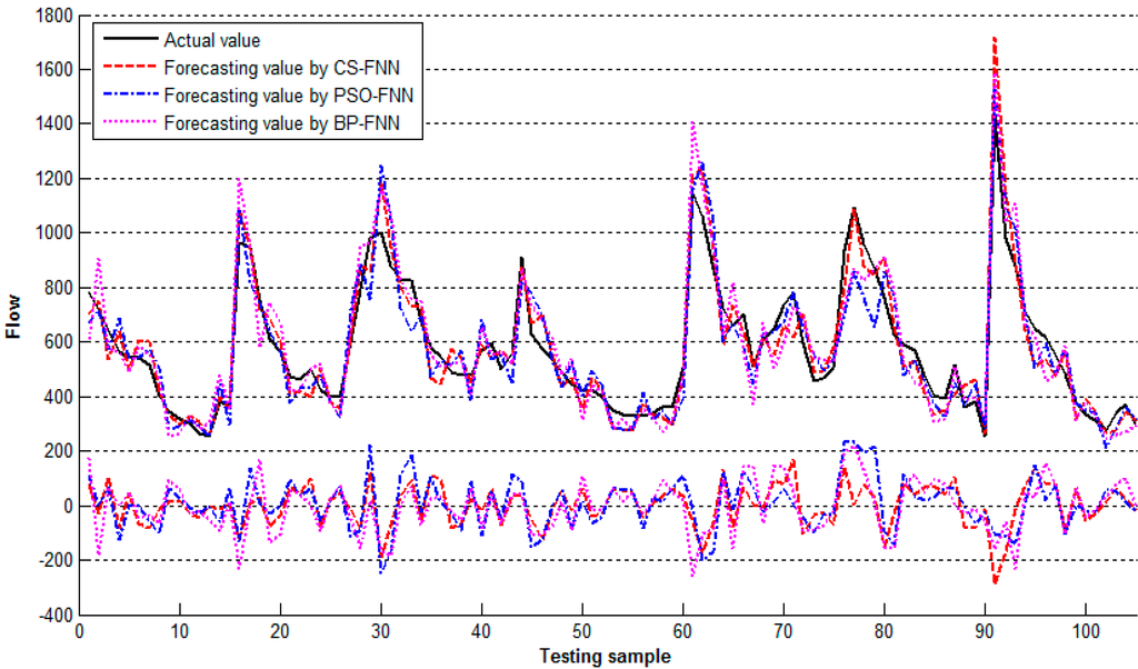
Figure 4.
The forecasting and actual values in the second scenario.
Table 3.
Performance statistics of the models on testing dataset in the third scenario.
| Model | RMSE | MAPE | R |
|---|---|---|---|
| BP-FNN | 76.1 | 0.108368 | 0.8737 |
| CS-FNN | 48.7161 | 0.067268 | 0.8965 |
| PSO-FNN | 66.9347 | 0.094968 | 0.8767 |
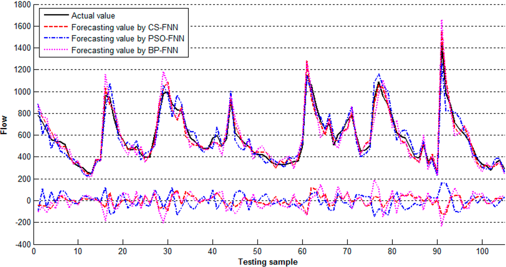
Figure 5.
The forecasting and actual values in the third scenario.
It was observed from Table 1, Table 2 and Table 3 that the CS-FNN has a smaller RMSE and MAPE as well as a bigger R in all scenarios than those of the BP-FNN and PSO-FNN. The results indicate that the proposed CS-FNN presents better performance in forecasting. The time series of actual and predicted values obtained using three different training algorithms are compared in Figure 3, Figure 4 and Figure 5. The nearly perfect agreement between the trends in the plots of the time series of actual and predicted values in these figures, obtained using different training algorithms, suggest that the FNN-based models used are appropriate for flow forecasting. However, when a high forecasting accuracy is sought, the FNN-CS is the most suitable model. Also, from tables and figures, the combination of inputs in the third scenario yielded the highest forecasting accuracy when compared with those in the first and second scenarios. The performance criteria RMSE, MAPE, and R obtained by the CS-FNN in the third scenario were calculated as 48.7161, 0.067268, and 0.8965, respectively. These results were highly correlated to the actual values. Theoretically, a forecasting model is accepted as ideal when MAPE is small and R is close to 1. The performance criteria indicate that the results obtained from the CS-FNN are satisfactory when compared with the results from studies on forecasting.
For the third scenario, the sensitivity analysis for the ANN models as per Garson’s method [47] was also conducted. Q(t) was found to be the most important input parameter, followed by X(t), Qday(t), Xday(t), Q(t−10), X(t−10), Q(t−20), and X(t−20).
Based on the obtained results, it can be concluded that the model based on CS-FNN can be accepted as a tool for forecasting flow.
7. Conclusions
Forecasting flow is important for water resource management and planning. In this study, different FNN-based models were developed and compared in order to forecast flow into the Hoabinh Reservoir. This study took advantage of a CS algorithm to train neural networks for hydrographic forecast problems. The CS algorithm was utilized for the training of feedforward neural networks. The obtained results showed that the neural network using CS performs well in all scenarios. The results of the CS-FNN were also compared against those of the BP-FNN and PSO-FNN in terms of RMSE, MAPE and R achieved. The CS-FNN was found to outperform the BP-FNN and PSO-FNN. These findings demonstrate the remarkable advantage of CS and the potential of ANNs in forecasting reservoir flows. The results of the present study also show that a comparative analysis of different training algorithms is always supportive in enhancing the performance of a neural network. This work can thus make a contribution to the development of the water resource reconcilement field. For future research, we will develop and incorporate our model in a user-friendly software tool in order to make this forecasting task easier.
Acknowledgment
This research was funded by the National Science Council of Taiwan under Grant No. NSC 102-2221-E-035-040.
Author Contributions
Quang Hung Do has initiated the idea of the work and written the manuscript. Jeng-Fung Chen conducted the literature review. Ho-Nien Hsieh collected the dataset. All of the authors have developed the research design and implemented the research. The final manuscript has been approved by all authors.
Nomenclature
| ACO | ant colony algorithm |
| ANN | artificial neural network |
| BP | back-propagation |
| CS | Cuckoo Search |
| FNN | feedforward neural network |
| GA | genetic algorithm |
| MAPE | mean absolute percentage error |
| MLP | multilayer perceptron |
| MLR | multiple linear regression |
| PSO | particle swarm optimization |
| R | correlation coefficient |
| RMSE | root mean square error |
Conflicts of Interest
The authors declare no conflict of interest.
References
- Kumar, K.V. Neural Network Prediction of Interfacial Tension at Crystal/Solution Interface. Ind. Eng. Chem. Res. 2009, 48, 4160–4164. [Google Scholar] [CrossRef]
- Chamkalani, A.; Zendehboudi, S.; Chamkalani, R.; Lohi, A.; Elkamel, A.; Chatzis, I. Utilization of support vector machine to calculate gas compressibility factor. Fluid Phase Equilib. 2013, 358, 189–202. [Google Scholar] [CrossRef]
- Shafiei, A.; Dusseault, M.B.; Zendehboudi, S.; Chatzis, I. A new screening tool for evaluation of steamflooding performance in Naturally Fractured Carbonate Reservoirs. Fuel 2013, 108, 502–514. [Google Scholar] [CrossRef]
- Roosta, A.; Setoodeh, P.; Jahanmiri, A. Artificial Neural Network Modeling of Surface Tension for Pure Organic Compounds. Ind. Eng. Chem. Res. 2011, 51, 561–566. [Google Scholar] [CrossRef]
- Zendehboudi, S.; Ahmadi, M.A.; Mohammadzadeh, O.; Bahadori, A.; Chatzis, I. Thermodynamic Investigation of Asphaltene Precipitation during Primary Oil Production: Laboratory and Smart Technique. Ind. Eng. Chem. Res. 2013, 52, 6009–6031. [Google Scholar] [CrossRef]
- Coulibaly, P.; Anctil, F.; Bobée, B. Multivariate Reservoir Inflow Forecasting Using Temporal Neural Networks. J. Hydrol. Eng. 2001, 6, 367–376. [Google Scholar] [CrossRef]
- Can, I.; Yerdelen, C.; Kahya1, E. Stochastic Modeling of Karasu River (Turkey) Using the Methods of Artificial Neural Networks. In Proceedings of the AGU Hydrology Days, Colorado, CO, USA, 19–21 March 2007; pp. 138–144.
- Dolling, O.R.; Varas, E.A. Artificial neural networks for stream flow prediction. J. Hydraul. Res. 2002, 40, 547–554. [Google Scholar] [CrossRef]
- Kilinş, I.; Ciğizouğlu, K. Reservoir Management Using Artificial Neural Networks. Available online: http://citeseerx.ist.psu.edu/viewdoc/summary?doi=10.1.1.104.174 (accessed on 31 October 2014).
- Lekkas, D.F.; Onof, C. Improved Flow Forecasting Using Artificial Neural Networks. In Proceedings of the 9th International Conference on Environmental Science and Technology, Rhodes island, Greece, 1–3 September 2005; pp. 877–884.
- Nguyen, V.H.; Cuong, T.H.; Pham, T.H.N. Hoabinh Reservoir Incoming Flow Forecast for the Period of 10 Days with Neural Networks. In Proceedings of Scientific Research in Open Universities’ HS-IC2007, CatBa, Vietnam, 4–6 November 2007; pp. 181–189.
- Sivapragasam, C.; Vanitha, S.; Muttil, N.; Suganya, K.; Suji, S.; Thamarai Selvi, M.; Selvi, R.; Jeya Sudha, S. Monthly flow forecast for Mississippi River basin using artificial neural networks. Neural Comput. Appl. 2014, 24, 1785–1793. [Google Scholar] [CrossRef]
- Hush, D.R.; Horne, B.G. Progress in supervised neural networks. IEEE Signal Process. Mag. 1993, 10, 8–39. [Google Scholar] [CrossRef]
- Hagar, M.T.; Menhaj, M.B. Training feedforward networks with the Marquardt algorithm. IEEE Trans. Neural Netw. 1994, 5, 989–993. [Google Scholar] [CrossRef]
- Adeli, H.; Hung, S.L. An adaptive conjugate gradient learning algorithm for efficient training of neural networks. Appl. Math. Comput. 1994, 62, 81–102. [Google Scholar] [CrossRef]
- Zhang, N. An online gradient method with momentum for two-layer feedforward neural networks. Appl. Math. Comput. 2009, 212, 488–498. [Google Scholar] [CrossRef]
- Mingguang, L.; Gaoyang, L. Artificial Neural Network Co-optimization Algorithm Based on Differential Evolution. In Proceedings of the Second International Symposium on Computational Intelligence and Design, Changsha, China, 12–14 December 2009; pp. 256–259.
- Gupta, J.N.D.; Sexton, R.S. Comparing backpropagation with a genetic algorithm for neural network training. Omega 1999, 27, 679–684. [Google Scholar] [CrossRef]
- Mirjalili, S.; Mohd Hashim, S.Z.; Moradian Sardroudi, H. Training feedforward neural networks using hybrid particle swarm optimization and gravitational search algorithm. Appl. Math. Comput. 2012, 218, 11125–11137. [Google Scholar] [CrossRef]
- Yang, X.S.; Deb, S. Cuckoo Search via Lévy Flights. In Proceedings of the World Congress on Nature and Biologically Inspired Computing (NaBIC), Coimbatore, India, 9–11 December 2009; pp. 210–214.
- Yang, X.-S.; Deb, S. Engineering optimisation by cuckoo search. Int. J. Math. Model. Numer. Optim. 2010, 1, 330–343. [Google Scholar]
- Yang, X.-S.; Deb, S.; Karamanoglu, M.; He, X. Cuckoo Search for Business Optimization Applications. In Proceedings of National Conference on Computing and Communication Systems (NCCCS), Durgapur, India, 21–22 November 2012; pp. 1–5.
- Kawam, A.A.L.; Mansour, N. Metaheuristic Optimization Algorithms for Training Artificial Neural Networks. Int. J. Comput. Inf. Technol. 2012, 1, 156–161. [Google Scholar]
- Valian, E.; Mohanna, S.; Tavakoli, S. Improved Cuckoo Search algorithm for feed forward neural network training. Int. J. Artif. Intell. Appl. 2011, 2, 36–43. [Google Scholar]
- Ünes, F. Prediction of Density Flow Plunging Depth in Dam Reservoirs: An Artificial Neural Network Approach. CLEAN Soil Air Water 2010, 38, 296–308. [Google Scholar] [CrossRef]
- Akhtar, M.K.; Corzo, G.A.; van Andel, S.J.; Jonoski, A. River flow forecasting with artificial neural networks using satellite observed precipitation pre-processed with flow length and travel time information: Case study of the Ganges river basin. Hydrol. Earth Syst. Sci. 2009, 13, 1607–1618. [Google Scholar] [CrossRef]
- Taghi Sattaria, M.; Yureklib, K.; Palc, M. Performance evaluation of artificial neural network approaches in forecasting reservoir inflow. Appl. Math. Model. 2012, 36, 2649–2657. [Google Scholar] [CrossRef]
- Huang, W.; Xu, B.; Chan-Hilton, A. Forecasting flows in Apalachicola River using neural networks. Hydrol. Process. 2004, 18, 2545–2564. [Google Scholar] [CrossRef]
- Gori, M.; Tesi, A. On the problem of local minima in back-propagation. IEEE Trans. Pattern Anal. Mach. Intell. 1992, 14, 76–86. [Google Scholar] [CrossRef]
- Zhang, J.R.; Zhang, J.; Lock, T.M.; Lyu, M.R. A hybrid particle swarm optimization—back-propagation algorithm for feedforward neural network training. Appl. Math. Comput. 2007, 185, 1026–1037. [Google Scholar] [CrossRef]
- Goldberg, D.E. Genetic Algorithms in Search, Optimization and Machine Learning; Addison Wesley: Boston, MA, USA, 1989. [Google Scholar]
- Kennedy, J.; Eberhart, R.C. Particle Swarm Optimization. In Proceedings of IEEE International Conference on Neural Networks, Perth, Australia, 27 November–1 December 1995; pp. 1942–1948.
- Dorigo, M.; Maniezzo, V.; Colorni, A. Ant system: Optimization by a colony of cooperating agents. IEEE Trans. Systems Man Cybern. Part B Cybern. 1996, 26, 29–41. [Google Scholar] [CrossRef]
- Mohamad, A.B.; Zain, A.M.; Bazin, N.E.N. Cuckoo Search Algorithm for Optimization Problems—A Literature Review and its Applications. Appl. Artif. Intell. 2014, 28, 419–448. [Google Scholar] [CrossRef]
- Yang, X.S.; Deb, S. Cuckoo search: Recent advances and applications. Neural Comput. Appl. 2014, 24, 169–174. [Google Scholar] [CrossRef]
- Yang, X.-S. (Ed.) Cuckoo Search and Firefly Algorithm; Springer: Berlin/Heidelberg, Germany, 2014.
- Walton, S.; Hassan, O.; Morgan, K.; Brown, M.R. Modified cuckoo search: A new gradient free optimization algorithm. Chaos Solitons Fractals 2011, 44, 710–718. [Google Scholar] [CrossRef]
- Walton, S.; Brown, M.R.; Hassan, O.; Morgan, K. Comment on Cuckoo search: A new nature-inspired optimization method for phase equilibrium calculations by V. Bhargava, S. Fateen, A. Bonilla-Petriciolet. Fluid Phase Equilib. 2013, 352, 64–66. [Google Scholar] [CrossRef]
- Funahashi, K. On the approximate realization of continuous mappings by neural networks. Neural Netw. 1989, 2, 183–192. [Google Scholar] [CrossRef]
- Norgaard, M.R.; Ravn, O.; Poulsen, N.K.; Hansen, L.K. Neural Networks for Modeling and Control of Dynamic Systems: A Practitioner’s Handbook; Springer: Berlin/Heidelberg, Germany, 2000. [Google Scholar]
- Caruana, R.; Lawrence, S.; Giles, C.L. Overfitting in Neural Networks: Backpropagation, Conjugate Gradient, and Early Stopping. In Proceedings of 13th Conference on Advances Neural Information Processing Systems, Vancouver, BC, Canada, 3–8 December 2001; pp. 402–408.
- Hornik, K.; Stinchombe, M.; White, H. Universal Approximation of an unknown Mapping and its Derivatives Using Multilayer Feed forward Networks. Neural Netw. 1990, 3, 551–560. [Google Scholar] [CrossRef]
- Cybenko, G. Approximation by superposition of a sigmoid function. Math. Control Signals Syst. 1989, 2, 303–314. [Google Scholar] [CrossRef]
- Bhattacharya, U.; Chaudhuri, B.B. Handwritten Numeral Databases of Indian Scripts and Multistage Recognition of Mixed Numerals. IEEE Trans. Pattern Anal. Mach. Intell. 2009, 31, 444–457. [Google Scholar] [CrossRef]
- Dogan, E.; Akgungor, A.P. Forecasting highway casualties under the effect of railway development policy in Turkey using artificial neural networks. Neural Comput. Appl. 2013, 22, 869–877. [Google Scholar] [CrossRef]
- MATLAB; R2014a; software for technical computation; The MathWorks, Inc.: Natick, MA, USA, 2014.
- Garson, G.D. Interpreting neural-network connection weights. AI Expert 1991, 6, 47–51. [Google Scholar]
© 2014 by the authors; licensee MDPI, Basel, Switzerland. This article is an open access article distributed under the terms and conditions of the Creative Commons Attribution license (http://creativecommons.org/licenses/by/4.0/).