
Extracting Self-Reported COVID-19 Symptom Tweets and Twitter Movement Mobility Origin/Destination Matrices to Inform Disease Models
 , , , and
Abstract
:1. Introduction
1.1. Related Works
1.2. Contribution and Structure
2. Data Collection
2.1. United Kingdom NHS Region-Specific Surveillance Data
2.1.1. Deaths
2.1.2. Hospital Admissions
2.1.3. Zoe App
2.1.4. 111 Calls and 111 Online
2.2. Symptomatic Tweets
- ·
- US: 50 States;
- ·
- Rest of the world: 2 European and 16 Latin American countries;
- ·
- UK: 7 NHS regions.
2.2.1. Pre-Processing Tweets
2.2.2. Symptom Classifier Breakdown
- Unrelated tweet;
- User currently has symptoms;
- User had symptoms in the past;
- Someone else currently has symptoms;
- Someone else had symptoms in the past.
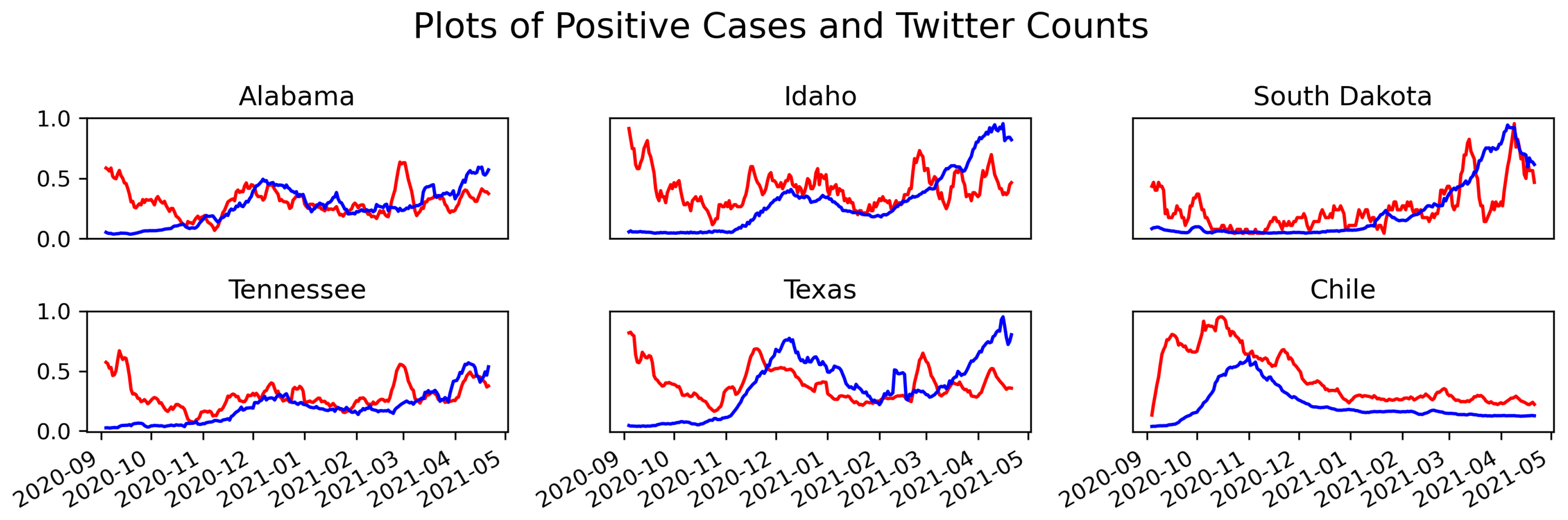
2.2.3. Comparison of Tweets and Positive Test Results
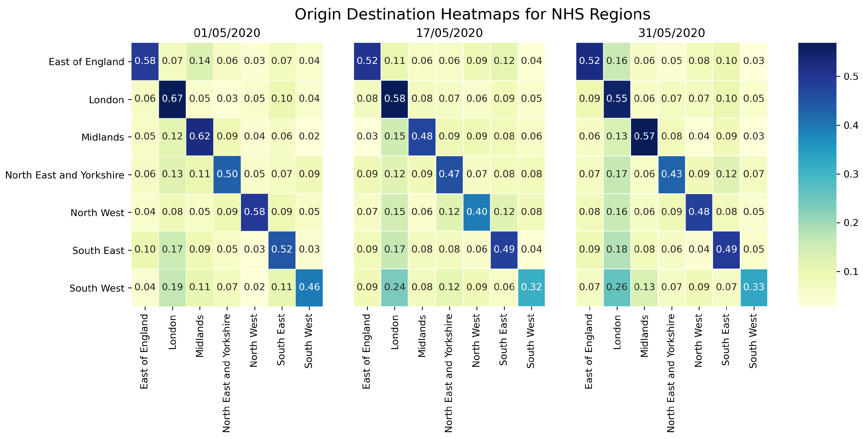
2.3. Twitter Mobility Origin Destination Matrices
3. Models
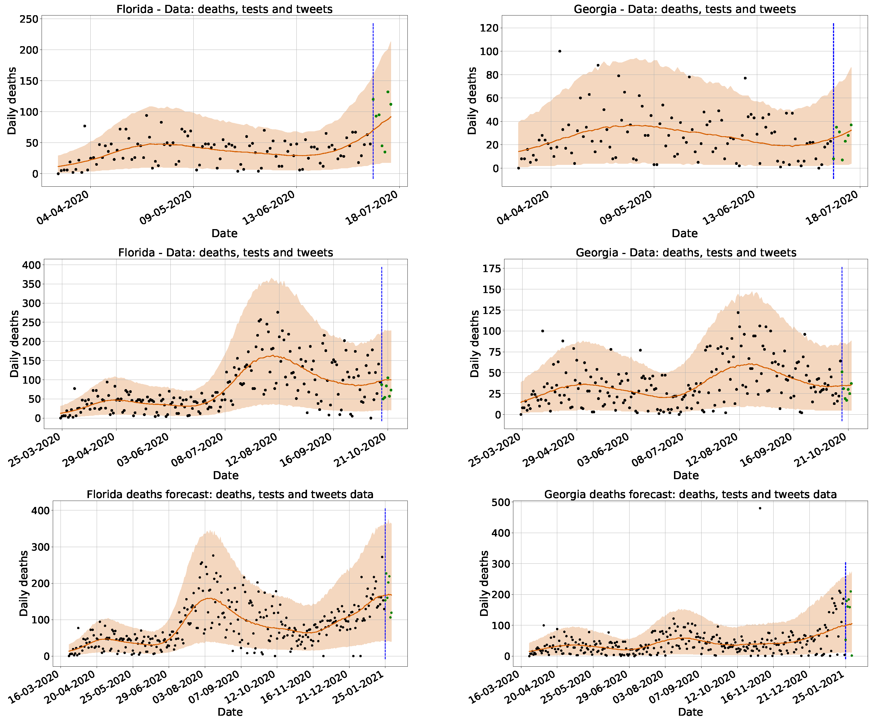
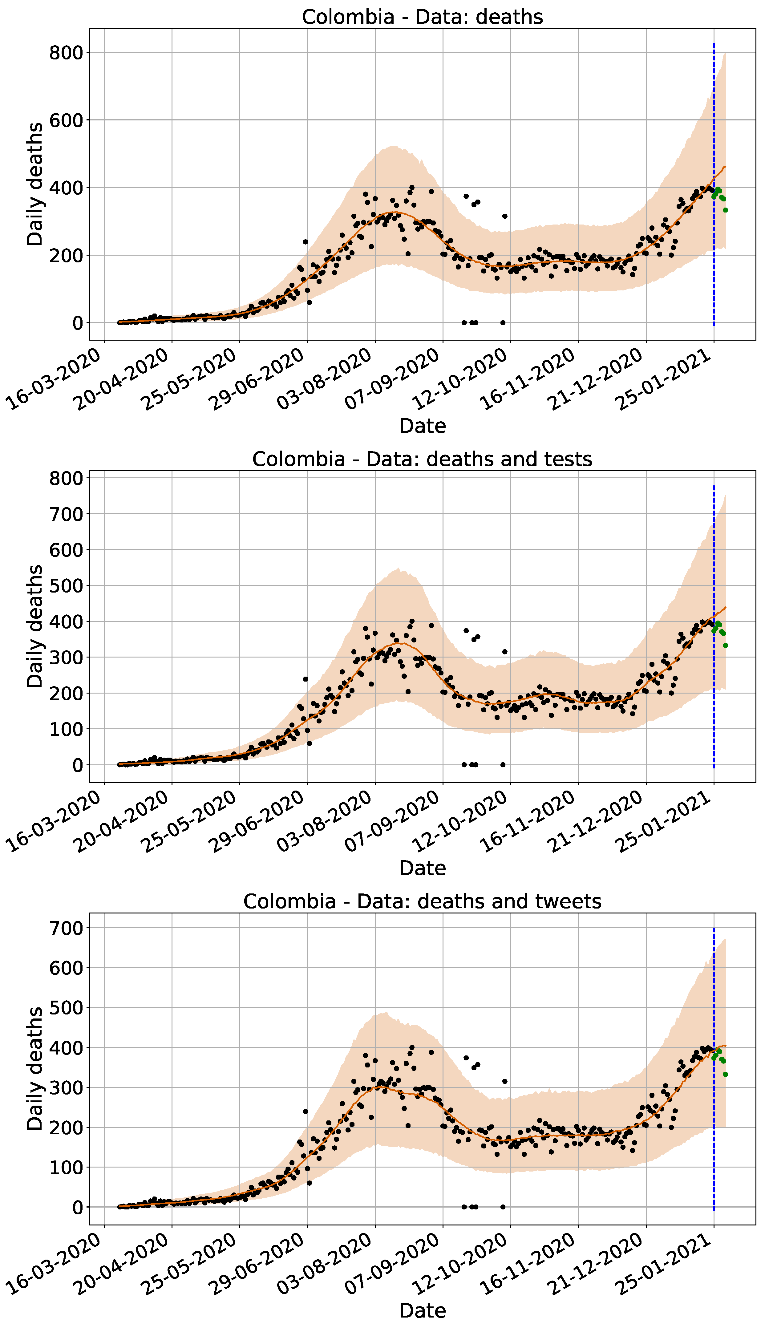
3.1. Model for Surveillance Data Comparison
3.1.1. Computational Experiments
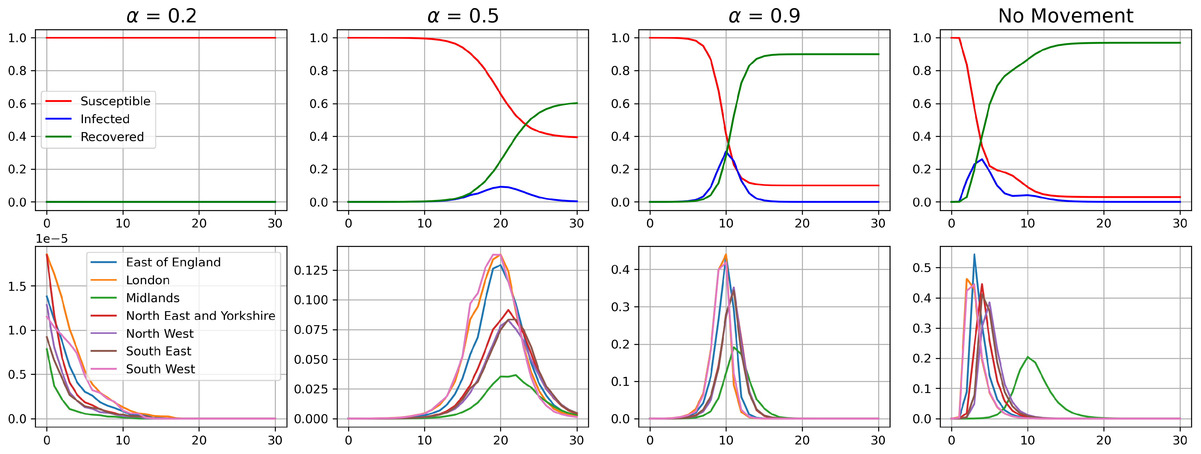
3.2. Model for Utilising Origin Destination Matrices
4. Results
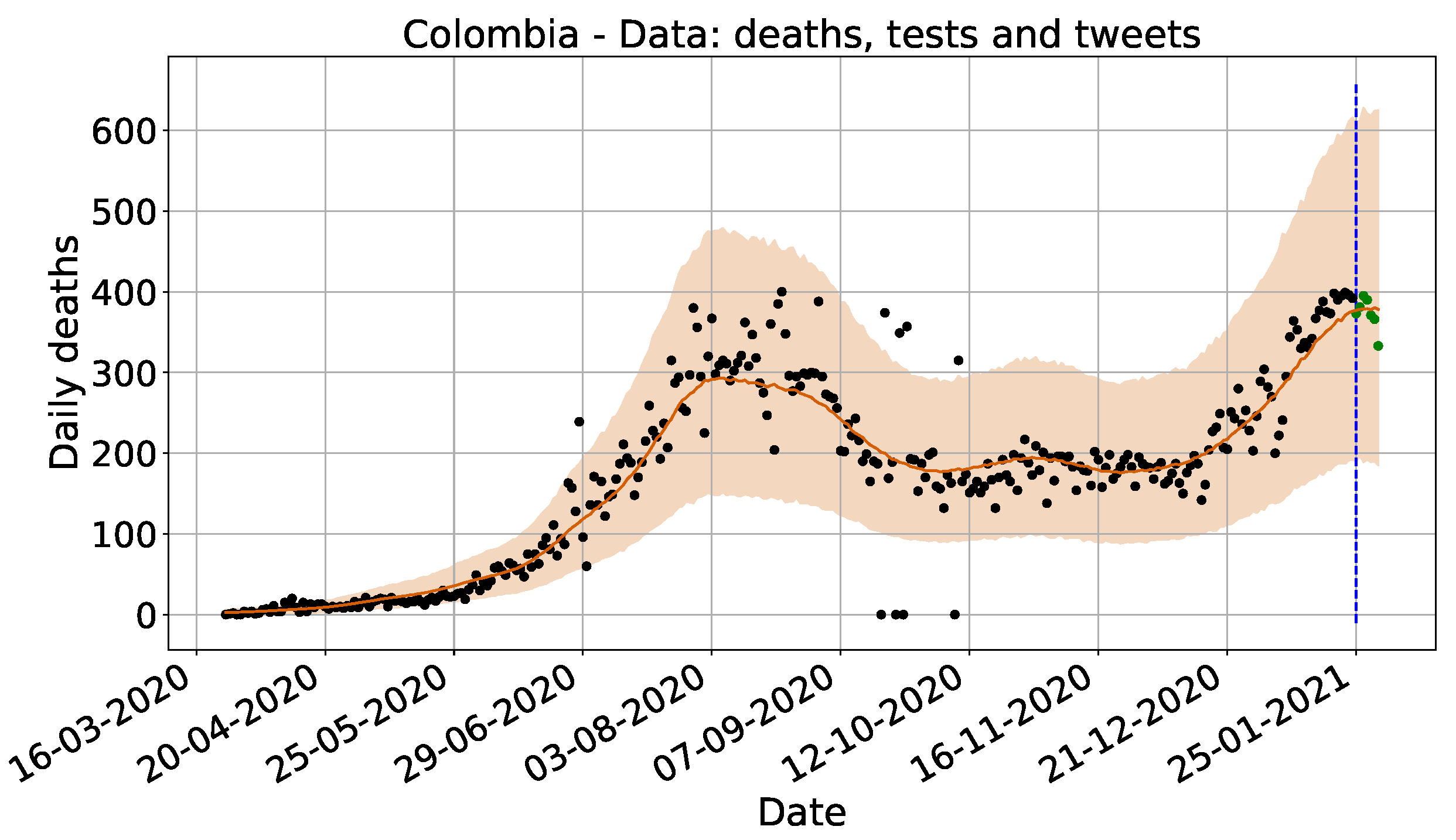
4.1. Surveillance Data Comparison
4.2. Origin Destination Matrices Analysis
5. Conclusions and Future Work
Author Contributions
Funding
Institutional Review Board Statement
Data Availability Statement
Acknowledgments
Conflicts of Interest
Abbreviations
| O/D | Origin/Destination |
| NHS | National Health Service |
| WHO | World Health Organisation |
| Reproduction Number | |
| UK | United Kingdom |
| ICU | Intensive Care Unit |
| NLP | Natural Language Processing |
| MAE | Mean Absolute Error |
| NEES | Normalised Estimation Error Squared |
| ROW | Rest of the World |
| JHU CSSE | Johns Hopkins University Center for Systems Science and Engineering |
| SVM | Support Vector Machine |
| NUTS | No-U-Turn Sampler |
| HPC | High-Performance Computer |
| BERT | Bidirectional Encoder Representations from Transformers |
Appendix A

| Geographic Location | Deaths | Tests | Tests and Twitter | ||||
|---|---|---|---|---|---|---|---|
| NEES | MAE % Diff | NEES | MAE % Diff | NEES | MAE % Diff | NEES | |
| Alaska | 0.329 | −36 | 0.334 | −29 | 0.301 | −92 | 0.302 |
| Alabama | 0.684 | −29 | 1.874 | −29 | 1.723 | −2 | 1.000 |
| Arkansas | 0.275 | 3 | 0.317 | −1 | 0.288 | −1 | 0.313 |
| Arizona | 0.337 | 20 | 0.334 | 18 | 0.344 | −20 | 0.244 |
| California | 0.611 | 6 | 0.709 | 9 | 0.802 | 5 | 1.206 |
| Colorado | 1.886 | −25 | 0.401 | −41 | 0.457 | 10 | 1.278 |
| Connecticut | 13.406 | −8 | 1.922 | −2 | 0.875 | 2 | 11.459 |
| Delaware | 3.020 | −3 | 0.918 | 16 | 1.046 | 12 | 0.727 |
| Florida | 0.406 | −24 | 0.179 | 13 | 0.353 | −20 | 0.454 |
| Georgia | 0.550 | 9 | 0.325 | 41 | 0.891 | −48 | 0.255 |
| Hawaii | 11.459 | −12 | 28.114 | −4 | 24.695 | 17 | 10.149 |
| Iowa | 19.176 | 5 | 7.720 | 4 | 1.476 | −3 | 1.600 |
| Idaho | 0.914 | 0 | 0.809 | 2 | 1.791 | 7 | 0.986 |
| Illinois | 0.573 | 9 | 0.350 | 13 | 0.319 | −116 | 1.091 |
| Indiana | 0.561 | −17 | 0.652 | −40 | 0.781 | 0 | 0.481 |
| Kansas | 1.021 | 1 | 1.037 | −2 | 1.835 | 1 | 0.488 |
| Kentucky | 0.355 | −4 | 0.374 | 10 | 0.548 | −15 | 0.214 |
| Louisiana | 0.298 | −7 | 0.305 | −2 | 0.341 | 9 | 0.234 |
| Massachusetts | 0.351 | 3 | 0.342 | −3 | 0.365 | 14 | 0.409 |
| Maryland | 0.485 | −3 | 0.619 | 10 | 0.581 | 31 | 0.313 |
| Maine | 0.488 | 1 | 0.567 | −28 | 0.796 | −9 | 0.952 |
| Michigan | 0.592 | −6 | 0.445 | −7 | 0.453 | 4 | 0.850 |
| Minnesota | 0.683 | 9 | 1.019 | 11 | 1.200 | 51 | 0.747 |
| Missouri | 0.810 | −7 | 1.165 | −27 | 1.609 | 20 | 0.475 |
| Mississippi | 0.683 | 12 | 0.721 | 2 | 0.997 | −15 | 0.320 |
| Montana | 5.034 | 4 | 2.244 | −1 | 1.538 | −5 | 5.189 |
| North Carolina | 0.908 | −1 | 0.453 | 9 | 0.877 | −19 | 0.570 |
| North Dakota | 0.513 | −32 | 0.521 | −18 | 0.544 | −8 | 0.661 |
| Nebraska | 0.259 | 5 | 0.253 | 7 | 0.570 | 5 | 0.286 |
| New Hampshire | 0.252 | −74 | 0.240 | −148 | 0.430 | −36 | 0.288 |
| New Jersey | 0.901 | −7 | 0.788 | −6 | 0.926 | 10 | 3.177 |
| New Mexico | 0.832 | −28 | 0.738 | −12 | 0.969 | 0 | 0.489 |
| Nevada | 2.129 | −24 | 0.353 | −12 | 0.425 | −13 | 1.904 |
| New York | 0.496 | 31 | 0.146 | 3 | 0.135 | −17 | 0.418 |
| Ohio | 0.263 | 63 | 0.675 | 54 | 0.468 | 3 | 0.337 |
| Oklahoma | 0.301 | −5 | 0.369 | 0 | 0.621 | 8 | 0.256 |
| Oregon | 0.729 | 0 | 1.032 | −2 | 1.692 | −4 | 0.793 |
| Pennsylvania | 0.411 | −7 | 0.385 | 0 | 0.426 | 10 | 0.402 |
| Rhode Island | 0.609 | −9 | 0.546 | −31 | 0.446 | −2 | 1.699 |
| South Carolina | 2.072 | −3 | 2.157 | −4 | 5.601 | −39 | 0.429 |
| South Dakota | 1.259 | 14 | 1.080 | −2 | 1.089 | 2 | 5.050 |
| Tennessee | 0.794 | 15 | 1.191 | 14 | 1.687 | −11 | 0.600 |
| Texas | 0.585 | 6 | 0.784 | 1 | 0.750 | −71 | 0.706 |
| Utah | 0.499 | −98 | 0.716 | −127 | 1.196 | 13 | 0.632 |
| Virginia | 0.731 | −10 | 0.396 | 6 | 0.864 | 9 | 0.676 |
| Vermont | 0.142 | 59 | 0.300 | −1 | 0.163 | 40 | 0.043 |
| Washington | 0.608 | −8 | 0.561 | 19 | 1.787 | −1 | 0.782 |
| Wisconsin | 0.842 | 6 | 1.028 | 25 | 3.921 | 8 | 0.850 |
| West Virginia | 0.650 | −6 | 0.547 | 2 | 1.042 | 7 | 0.291 |
| Wyoming | 1.939 | 5 | 0.951 | −15 | 1.126 | 25 | 0.395 |
| Average | 1.696 | −5 | 1.409 | −6 | 1.483 | −5 | 1.269 |
| Geographic Location | Language | Deaths | Tests | Tests and Twitter | ||||
|---|---|---|---|---|---|---|---|---|
| NEES | MAE % Diff | NEES | MAE % Diff | NEES | MAE % Diff | NEES | ||
| Argentina | Spanish | 0.567 | 3 | 0.695 | −17 | 0.904 | −19 | 0.765 |
| Bolivia | Spanish | 0.339 | −85 | 0.207 | −117 | 0.182 | −118 | 0.195 |
| Brazil | Portuguese | 0.396 | −4 | 0.405 | 11 | 0.578 | 4 | 0.493 |
| Chile | Spanish | 0.371 | 15 | 0.439 | 14 | 0.506 | 10 | 0.425 |
| Colombia | Spanish | 0.154 | 17 | 0.243 | −46 | 0.164 | −115 | 0.223 |
| Costa Rica | Spanish | 0.423 | 6 | 0.583 | 18 | 3.060 | 2 | 0.786 |
| Ecuador | Spanish | 0.156 | −26 | 0.195 | −99 | 0.234 | −69 | 0.234 |
| Guatemala | Spanish | 0.557 | −19 | 0.670 | −31 | 0.815 | −31 | 0.713 |
| Honduras | Spanish | 0.405 | −8 | 0.381 | −27 | 0.915 | −41 | 0.541 |
| Mexico | Spanish | 0.766 | 16 | 0.939 | 11 | 1.100 | 11 | 1.110 |
| Nicaragua | Spanish | 0.091 | −13 | 0.207 | −24 | 1.340 | −22 | 0.364 |
| Panama | Spanish | 0.550 | −20 | 0.421 | −4 | 0.451 | −7 | 0.368 |
| Paraguay | Spanish | 0.535 | 28 | 0.877 | −7 | 2.615 | 8 | 1.473 |
| Peru | Spanish | 0.507 | 33 | 0.103 | 26 | 1.630 | 16 | 0.515 |
| Uruguay | Spanish | 0.619 | 11 | 0.742 | −13 | 0.899 | −7 | 0.643 |
| Venezuela | Spanish | 0.610 | −14 | 0.713 | −49 | 0.890 | −91 | 0.603 |
| Germany | German | 0.379 | 5 | 0.613 | 15 | 2.131 | 14 | 1.570 |
| Italy | Italian | 0.360 | 17 | 0.557 | 29 | 3.149 | 34 | 1.991 |
| Average | 0.433 | −6 | 0.500 | −17 | 1.198 | −24 | 0.723 | |
| Geographic Location | Deaths | Hospital | Zoe App | 111 Calls | 111 Online | ||||||
|---|---|---|---|---|---|---|---|---|---|---|---|
| NEES | MAE % Diff | NEES | MAE % Diff | NEES | MAE % Diff | NEES | MAE % Diff | NEES | MAE % Diff | NEES | |
| East of England | 0.435 | −13 | 0.419 | −7 | 0.655 | 38 | 2.908 | −15 | 0.820 | −19 | 0.795 |
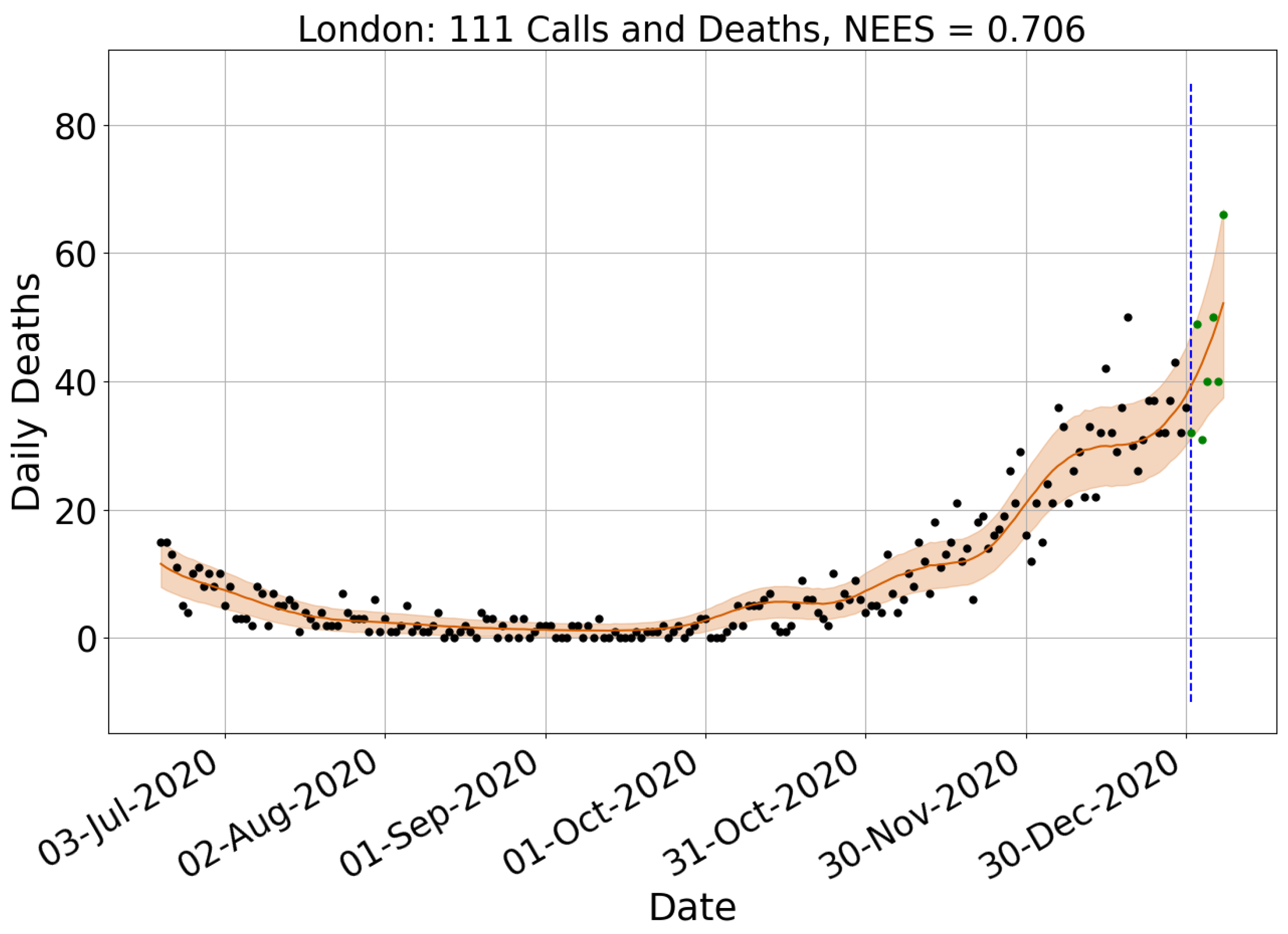
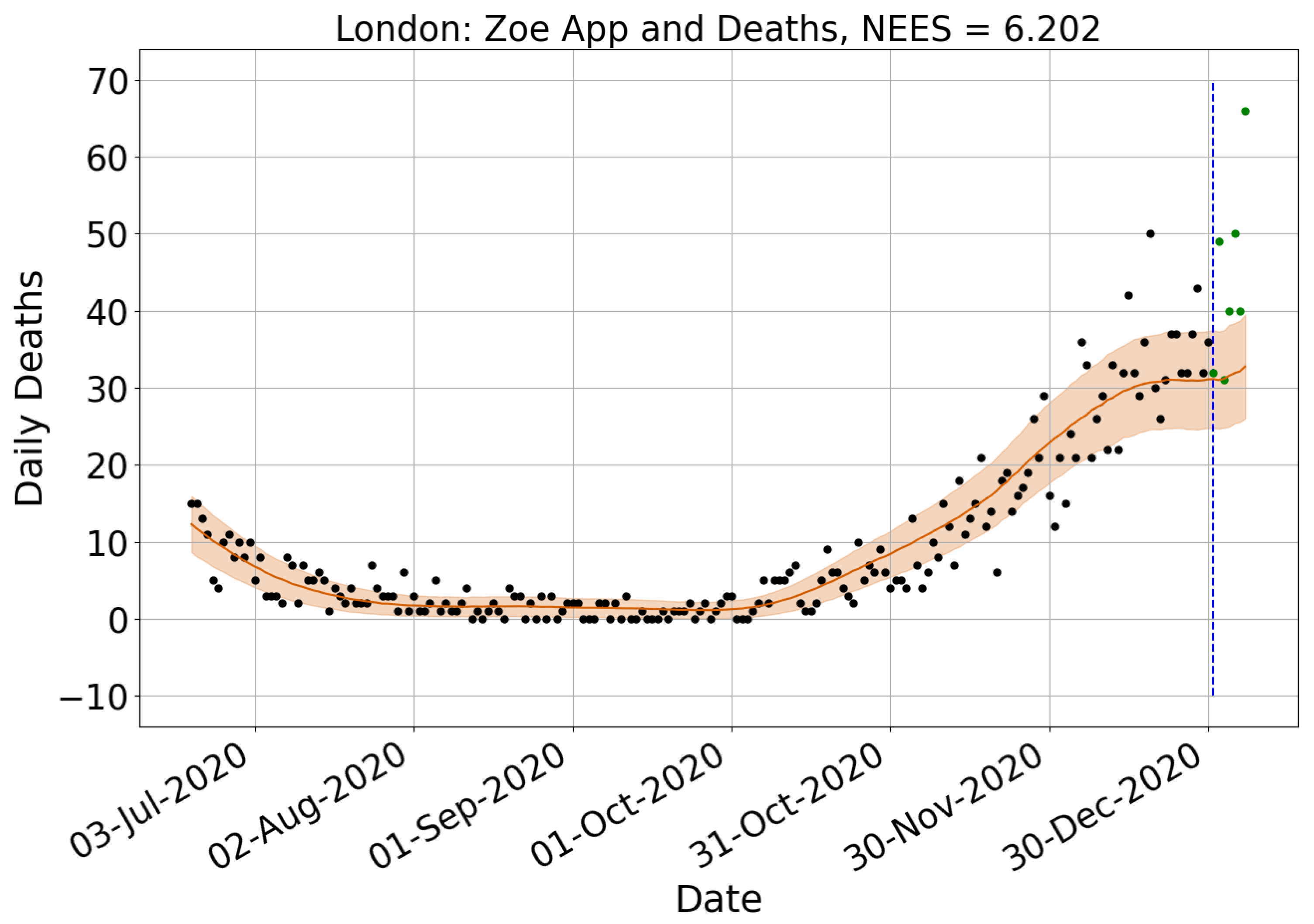
| London | 0.878 | −36 | 0.666 | −7 | 1.163 | 131 | 3.150 | −43 | 0.750 | −47 | 0.754 |
| Midlands | 0.635 | −16 | 0.466 | 13 | 0.569 | 132 | 3.330 | −19 | 0.418 | −47 | 0.404 |
| North East and Yorkshire | 0.753 | 5 | 1.188 | −4 | 0.824 | 153 | 2.325 | −16 | 0.860 | −14 | 0.888 |
| North West | 0.735 | −1 | 0.756 | 17 | 1.408 | 129 | 3.285 | −25 | 0.932 | −25 | 0.934 |
| South East | 0.652 | −24 | 0.805 | −3 | 1.255 | 126 | 4.390 | 8 | 1.018 | 6 | 0.957 |
| South West | 0.545 | −69 | 0.474 | 2 | 1.432 | 160 | 2.729 | −8 | 1.617 | −6 | 1.653 |
| Average | 0.662 | −22 | 0.682 | 2 | 1.044 | 124 | 3.160 | −17 | 0.916 | −22 | 0.912 |
References
- Coronavirus Disease 2019. Available online: https://www.google.com/search?q=covid-19+cases+worldwide&rlz=1C1CHBF_enGB763GB763&sxsrf=AJOqlzVAHRTMaItK2GPe9r5WtVyiju1d9g%3A1677849490518&ei=kvMBZO6lH4SW8gL377G4Dg&ved=0ahUKEwjutvm27L_9AhUEi1wKHfd3DOcQ4dUDCA8&uact=5&oq=covid-19+cases+worldwide&gs_lcp=Cgxnd3Mtd2l6LXNlcnAQAzIFCAAQgAQyBQgAEIAEMgYIABAWEB4yBggAEBYQHjIGCAAQFhAeMgYIABAWEB4yBggAEBYQHjIGCAAQFhAeMgYIABAWEB4yBggAEBYQHjoKCAAQRxDWBBCwAzoECAAQQ0oECEEYAFDLBFjOEWCFEmgBcAB4AIABWIgB8QSSAQE5mAEAoAEByAEIwAEB&sclient=gws-wiz-serpt (accessed on 3 March 2023).
- Dong, E.; Du, H.; Gardner, L. An interactive web-based dashboard to track COVID-19 in real time. Lancet Infect. Dis. 2020, 20, 533–534. [Google Scholar] [CrossRef] [PubMed]
- Kermack, W.O.; McKendrick, A.G. A contribution to the mathematical theory of epidemics. Proc. R. Soc. London. Ser. A Contain Pap. Math. Phys. Charact. 1927, 115, 700–721. [Google Scholar]
- Reproduction Number (R) and Growth Rate: Methodology. Available online: https://www.gov.uk/government/publications/reproduction-number-r-and-growth-rate-methodology/reproduction-number-r-and-growth-rate-methodology (accessed on 1 October 2021).
- Birrell, P.; Blake, J.; Van Leeuwen, E.; Gent, N.; De Angelis, D. Real-time nowcasting and forecasting of COVID-19 dynamics in England: The first wave. Philos. Trans. R. Soc. B 2021, 376, 20200279. [Google Scholar] [CrossRef] [PubMed]
- Leclerc, Q.J.; Nightingale, E.S.; Abbott, S.; Jombart, T. Analysis of temporal trends in potential COVID-19 cases reported through NHS Pathways England. Sci. Rep. 2021, 11, 34053254. [Google Scholar] [CrossRef]
- Keeling, M.J.; Dyson, L.; Guyver-Fletcher, G.; Holmes, A.; Semple, M.G.; Investigators, I.; Tildesley, M.J.; Hill, E.M. Fitting to the UK COVID-19 outbreak, short-term forecasts and estimating the reproductive number. Stat. Methods Med. Res. 2022, 2022, 09622802211070257. [Google Scholar] [CrossRef]
- Moore, R.E.; Rosato, C.; Maskell, S. Refining epidemiological forecasts with simple scoring rules. Philos. Trans. R. Soc. A 2022, 380, 20210305. [Google Scholar] [CrossRef]
- Funk, S.; Abbott, S.; Atkins, B.D.; Baguelin, M.; Baillie, J.K.; Birrell, P.; Blake, J.; Bosse, N.I.; Burton, J.; Carruthers, J.; et al. Short-term forecasts to inform the response to the Covid-19 epidemic in the UK. MedRxiv 2020. [Google Scholar] [CrossRef]
- Overton, C.E.; Pellis, L.; Stage, H.B.; Scarabel, F.; Burton, J.; Fraser, C.; Hall, I.; House, T.A.; Jewell, C.; Nurtay, A.; et al. EpiBeds: Data informed modelling of the COVID-19 hospital burden in England. PLoS Comput. Biol. 2022, 18, e1010406. [Google Scholar] [CrossRef]
- Czado, C.; Gneiting, T.; Held, L. Predictive model assessment for count data. Biometrics 2009, 65, 1254–1261. [Google Scholar] [CrossRef]
- Aramaki, E.; Maskawa, S.; Morita, M. Twitter catches the flu: Detecting influenza epidemics using Twitter. In Proceedings of the 2011 Conference on Empirical Methods in Natural Language Processing, Edinburgh, UK, 27–31 July 2011; pp. 1568–1576. [Google Scholar]
- Aslam, A.A.; Tsou, M.H.; Spitzberg, B.H.; An, L.; Gawron, J.M.; Gupta, D.K.; Peddecord, K.M.; Nagel, A.C.; Allen, C.; Yang, J.A.; et al. The reliability of tweets as a supplementary method of seasonal influenza surveillance. J. Med. Internet Res. 2014, 16, e3532. [Google Scholar] [CrossRef]
- Broniatowski, D.A.; Paul, M.J.; Dredze, M. National and local influenza surveillance through Twitter: An analysis of the 2012–2013 influenza epidemic. PLoS ONE 2013, 8, e83672. [Google Scholar] [CrossRef] [PubMed] [Green Version]
- Eysenbach, G. Infodemiology and infoveillance: Framework for an emerging set of public health informatics methods to analyze search, communication and publication behavior on the Internet. J. Med. Internet Res. 2009, 11, e1157. [Google Scholar] [CrossRef] [PubMed]
- Achrekar, H.; Gandhe, A.; Lazarus, R.; Yu, S.H.; Liu, B. Predicting flu trends using twitter data. In Proceedings of the 2011 IEEE Conference on Computer Communications Workshops (INFOCOM WKSHPS), Toronto, ON, Canada, 10–15 April 2011; pp. 702–707. [Google Scholar]
- Șerban, O.; Thapen, N.; Maginnis, B.; Hankin, C.; Foot, V. Real-time processing of social media with SENTINEL: A syndromic surveillance system incorporating deep learning for health classification. Inf. Process. Manag. 2019, 56, 1166–1184. [Google Scholar]
- Espinosa, L.; Wijermans, A.; Orchard, F.; Höhle, M.; Czernichow, T.; Coletti, P.; Hermans, L.; Faes, C.; Kissling, E.; Mollet, T. Epitweetr: Early warning of public health threats using Twitter data. Eurosurveillance 2022, 27, 2200177. [Google Scholar] [CrossRef]
- Lamsal, R.; Harwood, A.; Read, M.R. Twitter conversations predict the daily confirmed COVID-19 cases. Appl. Soft Comput. 2022, 129, 109603. [Google Scholar] [CrossRef]
- Thakur, N. A Large-Scale Dataset of Twitter Chatter about Online Learning during the Current COVID-19 Omicron Wave. Data 2022, 7, 109. [Google Scholar] [CrossRef]
- Thakur, N.; Han, C.Y. An Exploratory Study of Tweets about the SARS-CoV-2 Omicron Variant: Insights from Sentiment Analysis, Language Interpretation, Source Tracking, Type Classification, and Embedded URL Detection. COVID 2022, 2, 1026–1049. [Google Scholar] [CrossRef]
- Medford, R.J.; Saleh, S.N.; Sumarsono, A.; Perl, T.M.; Lehmann, C.U. An “infodemic”: Leveraging high-volume Twitter data to understand early public sentiment for the coronavirus disease 2019 outbreak. In Proceedings of the Open Forum Infectious Diseases; Oxford University Press: Oxford, MI, USA, 2020; Volume 7, p. ofaa258. [Google Scholar]
- Zhang, Y.; Lyu, H.; Liu, Y.; Zhang, X.; Wang, Y.; Luo, J. Monitoring depression trends on twitter during the COVID-19 pandemic: Observational study. JMIR Infodemiol. 2021, 1, e26769. [Google Scholar] [CrossRef]
- Lwin, M.O.; Lu, J.; Sheldenkar, A.; Schulz, P.J.; Shin, W.; Gupta, R.; Yang, Y. Global sentiments surrounding the COVID-19 pandemic on Twitter: Analysis of Twitter trends. JMIR Public Health Surveill. 2020, 6, e19447. [Google Scholar] [CrossRef]
- Sharma, K.; Seo, S.; Meng, C.; Rambhatla, S.; Liu, Y. COVID-19 on social media: Analyzing misinformation in twitter conversations. arXiv 2020, arXiv:2003.12309. [Google Scholar]
- Al-Garadi, M.A.; Yang, Y.C.; Lakamana, S.; Sarker, A. A Text Classification Approach for the Automatic Detection of Twitter Posts Containing Self-Reported COVID-19 Symptoms. 2020. Available online: https://openreview.net/forum?id=xyGSIttHYO (accessed on 6 March 2023).
- Sarker, A.; Lakamana, S.; Hogg-Bremer, W.; Xie, A.; Al-Garadi, M.A.; Yang, Y.C. Self-reported COVID-19 symptoms on Twitter: An analysis and a research resource. J. Am. Med. Inform. Assoc. 2020, 27, 1310–1315. [Google Scholar] [CrossRef] [PubMed]
- Garcia, K.; Berton, L. Topic detection and sentiment analysis in Twitter content related to COVID-19 from Brazil and the USA. Appl. Soft Comput. 2021, 101, 107057. [Google Scholar] [CrossRef] [PubMed]
- Kar, D.; Bhardwaj, M.; Samanta, S.; Azad, A.P. No rumours please! A multi-indic-lingual approach for COVID fake-tweet detection. In Proceedings of the 2021 Grace Hopper Celebration India (GHCI), Bangalore, India, 18 January–3 February 2021; pp. 1–5. [Google Scholar]
- Badr, H.S.; Du, H.; Marshall, M.; Dong, E.; Squire, M.M.; Gardner, L.M. Association between mobility patterns and COVID-19 transmission in the USA: A mathematical modelling study. Lancet Infect. Dis. 2020, 20, 1247–1254. [Google Scholar] [CrossRef] [PubMed]
- Goel, R.; Sharma, R. Mobility based sir model for pandemics-with case study of covid-19. In Proceedings of the 2020 IEEE/ACM International Conference on Advances in Social Networks Analysis and Mining (ASONAM), The Hague, The Netherlands, 7–10 December 2020; pp. 110–117. [Google Scholar]
- Osorio-Arjona, J.; García-Palomares, J.C. Social media and urban mobility: Using twitter to calculate home-work travel matrices. Cities 2019, 89, 268–280. [Google Scholar] [CrossRef]
- Huang, X.; Li, Z.; Jiang, Y.; Li, X.; Porter, D. Twitter reveals human mobility dynamics during the COVID-19 pandemic. PLoS ONE 2020, 15, e0241957. [Google Scholar] [CrossRef]
- Lombardi, A.; Amoroso, N.; Monaco, A.; Tangaro, S.; Bellotti, R. Complex Network Modelling of Origin–Destination Commuting Flows for the COVID-19 Epidemic Spread Analysis in Italian Lombardy Region. Appl. Sci. 2021, 11, 4381. [Google Scholar] [CrossRef]
- Gómez, S.; Fernández, A.; Meloni, S.; Arenas, A. Impact of origin-destination information in epidemic spreading. Sci. Rep. 2019, 9, 2315. [Google Scholar] [CrossRef] [Green Version]
- Kondo, K. Simulating the impacts of interregional mobility restriction on the spatial spread of COVID-19 in Japan. Sci. Rep. 2021, 11, 18951. [Google Scholar] [CrossRef]
- Flaxman, S.; Mishra, S.; Gandy, A.; Unwin, H.J.T.; Mellan, T.A.; Coupland, H.; Whittaker, C.; Zhu, H.; Berah, T.; Eaton, J.W.; et al. Estimating the effects of non-pharmaceutical interventions on COVID-19 in Europe. Nature 2020, 584, 257–261. [Google Scholar] [CrossRef]
- Vinceti, M.; Filippini, T.; Rothman, K.J.; Ferrari, F.; Goffi, A.; Maffeis, G.; Orsini, N. Lockdown timing and efficacy in controlling COVID-19 using mobile phone tracking. EClinicalMedicine 2020, 25, 100457. [Google Scholar] [CrossRef]
- CoDatMo. 2021 Welcome to the CoDatMo Site. Available online: https://codatmo.github.io (accessed on 1 October 2021).
- UK Government. 2021 Coronavirus (COVID-19) in the UK. Available online: https://coronavirus.data.gov.uk/details/deaths (accessed on 1 October 2021).
- UK Government. 2021 Coronavirus (COVID-19) in the UK. Available online: https://coronavirus.data.gov.uk/details/healthcare (accessed on 1 October 2021).
- Zoe App: COVID-Public-Data. Available online: https://console.cloud.google.com/storage/browser/covid-public-data;tab=objects?prefix=&forceOnObjectsSortingFiltering=false (accessed on 1 October 2021).
- Potential Coronavirus (COVID-19) Symptoms Reported through NHS Pathways and 111 Online. Available online: https://digital.nhs.uk/data-and-information/publications/statistical/mi-potential-covid-19-symptoms-reported-through-nhs-pathways-and-111-online/latest (accessed on 1 October 2021).
- Roesslein, J. Tweepy Documentation. 2009, Volume 5, p. 724. Available online: http://tweepy.readthedocs.io/en/v3 (accessed on 8 May 2012).
- COVID-19 Terms and MedDRA. Available online: https://www.meddra.org/COVID-19-terms-and-MedDRA (accessed on 1 October 2021).
- Pedregosa, F.; Varoquaux, G.; Gramfort, A.; Michel, V.; Thirion, B.; Grisel, O.; Blondel, M.; Prettenhofer, P.; Weiss, R.; Dubourg, V.; et al. Scikit-learn: Machine learning in Python. J. Mach. Learn. Res. 2011, 12, 2825–2830. [Google Scholar]
- Leetaru, K.; Wang, S.; Cao, G.; Padmanabhan, A.; Shook, E. Mapping the global Twitter heartbeat: The geography of Twitter. First Monday 2013. Available online: https://journals.uic.edu/ojs/index.php/fm/article/view/4366 (accessed on 1 October 2021). [CrossRef]
- Carpenter, B.; Gelman, A.; Hoffman, M.D.; Lee, D.; Goodrich, B.; Betancourt, M.; Brubaker, M.; Guo, J.; Li, P.; Riddell, A. Stan: A probabilistic programming language. J. Stat. Softw. 2017, 76, 1430202. [Google Scholar] [CrossRef] [PubMed] [Green Version]
- Hoffman, M.D.; Gelman, A. The No-U-Turn sampler: Adaptively setting path lengths in Hamiltonian Monte Carlo. J. Mach. Learn. Res. 2014, 15, 1593–1623. [Google Scholar]
- Chen, Z.; Heckman, C.; Julier, S.; Ahmed, N. Weak in the NEES?: Auto-tuning Kalman filters with Bayesian optimization. In Proceedings of the 2018 21st International Conference on Information Fusion (FUSION), Cambridge, UK, 10–13 July 2018; pp. 1072–1079. [Google Scholar]
- Modelling the Coronavirus Epidemic in a City with Python. Available online: https://towardsdatascience.com/modelling-the-coronavirus-epidemic-spreading-in-a-city-with-python-babd14d82fa2 (accessed on 24 October 2022).
- Wesolowski, A.; zu Erbach-Schoenberg, E.; Tatem, A.J.; Lourenço, C.; Viboud, C.; Charu, V.; Eagle, N.; Engø-Monsen, K.; Qureshi, T.; Buckee, C.O.; et al. Multinational patterns of seasonal asymmetry in human movement influence infectious disease dynamics. Nat. Commun. 2017, 8, 2069. [Google Scholar] [CrossRef] [PubMed] [Green Version]
- Huang, C.Y.; Tong, H.; He, J.; Maciejewski, R. Location Prediction for Tweets. Front. Big Data 2019, 2, 5. [Google Scholar] [CrossRef] [PubMed] [Green Version]
- Devlin, J.; Chang, M.W.; Lee, K.; Toutanova, K. Bert: Pre-training of deep bidirectional transformers for language understanding. arXiv 2018, arXiv:1810.04805. [Google Scholar]
- Del Moral, P.; Doucet, A.; Jasra, A. Sequential monte carlo samplers. J. R. Stat. Soc. Ser. (Statist. Methodol.) 2006, 68, 411–436. [Google Scholar] [CrossRef] [Green Version]
- Devlin, L.; Horridge, P.; Green, P.L.; Maskell, S. The No-U-Turn sampler as a proposal distribution in a sequential Monte Carlo sampler with a near-optimal L-kernel. arXiv 2021, arXiv:2108.02498. [Google Scholar]


| Geographic Location | Data Feed | Start Date | Reference |
|---|---|---|---|
| U.S States and the rest of the world | Deaths | 24 March 2020 | [2] |
| Tests | 1 March 2020 | [2] | |
| 13 April 2020 | Section 2.2 | ||
| U.K NHS Regions | Deaths | 24 March 2020 | [40] |
| Hospital admissions | 19 March 2020 | [41] | |
| 9 April 2020 | Section 2.2 | ||
| Zoe app | 12 May 2020 | [42] | |
| 111 calls | 18 March 2020 | [43] | |
| 111 online | 18 March 2020 | [43] |
| Language | Number of Data Used | Performance Measures | ||||
|---|---|---|---|---|---|---|
| Training | Testing | F1 | Accuracy | Precision | Recall | |
| English | 1105 | 195 | 0.85 | 0.85 | 0.85 | 0.85 |
| German | 412 | 260 | 0.89 | 0.89 | 0.90 | 0.89 |
| Italian | 254 | 260 | 0.97 | 0.96 | 0.97 | 0.96 |
| Portuguese | 3507 | 619 | 0.77 | 0.77 | 0.78 | 0.80 |
| Spanish | 1530 | 270 | 0.82 | 0.85 | 0.82 | 0.85 |
| US States and the Rest of the World | NHS Regions |
|---|---|
| 9 July 2020–16 July 2020 | 11 November 2020–18 November 2020 |
| 17 October 2020–24 October 2020 | 21 November 2020–28 November 2020 |
| 25 January 2021–1 February 2021 | 1 December 2020–8 December 2020 |
| - | 11 December 2020–18 December 2020 |
| - | 21 December 2020–28 December 2020 |
| - | 31 December 2020–7 January 2021 |
Disclaimer/Publisher’s Note: The statements, opinions and data contained in all publications are solely those of the individual author(s) and contributor(s) and not of MDPI and/or the editor(s). MDPI and/or the editor(s) disclaim responsibility for any injury to people or property resulting from any ideas, methods, instructions or products referred to in the content. |
© 2023 by the authors. Licensee MDPI, Basel, Switzerland. This article is an open access article distributed under the terms and conditions of the Creative Commons Attribution (CC BY) license (https://creativecommons.org/licenses/by/4.0/).
Share and Cite
Rosato, C.; Moore, R.E.; Carter, M.; Heap, J.; Harris, J.; Storopoli, J.; Maskell, S. Extracting Self-Reported COVID-19 Symptom Tweets and Twitter Movement Mobility Origin/Destination Matrices to Inform Disease Models. Information 2023, 14, 170. https://doi.org/10.3390/info14030170
Rosato C, Moore RE, Carter M, Heap J, Harris J, Storopoli J, Maskell S. Extracting Self-Reported COVID-19 Symptom Tweets and Twitter Movement Mobility Origin/Destination Matrices to Inform Disease Models. Information. 2023; 14(3):170. https://doi.org/10.3390/info14030170
Chicago/Turabian StyleRosato, Conor, Robert E. Moore, Matthew Carter, John Heap, John Harris, Jose Storopoli, and Simon Maskell. 2023. "Extracting Self-Reported COVID-19 Symptom Tweets and Twitter Movement Mobility Origin/Destination Matrices to Inform Disease Models" Information 14, no. 3: 170. https://doi.org/10.3390/info14030170