New Equations to Evaluate Lateral Displacement Caused by Liquefaction Using the Response Surface Method

Abstract

Few empirical and semi-empirical approaches have considered the influence of the geology, tectonic source, causative fault type, and frequency content of earthquake motion on lateral displacement caused by liquefaction (D_H). This paper aims to address this gap in the literature by adding an earthquake parameter of the standardized cumulative absolute velocity (CAV₅) to the original dataset for analyzing. Furthermore, the complex influence of fine content in the liquefiable layer (F₁₅) is analyzed by deriving two different equations: the first one is for the whole range of parameters, and the second one is for a limited range of F₁₅ values under 28% in order to the F₁₅’s critical value presented in literature. The new response surface method (RSM) approach is applied on the basis of the artificial neural network (ANN) model to develop two new equations. Moreover, to illustrate the capability and efficiency of the developed models, the results of the RSM models are examined by comparing them with an additional three available models using data from the Chi-Chi earthquake sites that were not used for developing the models in this study. In conclusion, the RSM provides a capable tool to evaluate the liquefaction phenomenon, and the results fully justify the complex effect of different values of F₁₅.

1. Introduction

When, during earthquake motion, pore water pressure rises because of applied dynamic loads, the loose saturated sand layer that is relatively close to the ground surface is liquefied. Liquefaction can be discovered through manifestations such as (1) a sharp decrease in the frequency content of a sand layer, (2) settlement, (3) flow slides, (4) sand boiling, (5) foundation failure, and (6) lateral displacement (D_H).

The movements of sand blocks, which have destroyed and affected constructions and infrastructure, ranging from a few centimeters to some meters [1], have been reported. Lateral displacement can be significantly damaging for piles, piers, and pipe lines during and for a short time after earthquakes and causes more damage to structures and infrastructures than any other type of liquefaction-induced ground failure. In this phenomenon, the large blocks of soil move towards the free face or along the slope. Researchers have developed several different models and approaches to predict the D_H caused by liquefaction for some decades. Some of them have proposed numerical approaches [2,3,4,5,6] such as the finite element method (FEM) and the finite difference method (FDM). Next to that, analytical approaches have been developed, for example, minimum potential energy [7] and the sliding block model [8,9,10,11,12].

Among them, due to the complicated input model parameters and difficulties in their calculations, as well as because of the complex mechanism of liquefaction, empirical and semi-empirical models are the most common models that have been performed and developed by engineers and researchers [13,14,15,16,17]. However, in most cases, because of the scarcity and shortage in their database, some aspects of this phenomenon, such as geology, fault type, and the effect of near-fault sites, have been ignored, with the exception of Zhang et al. [18], who used Japanese spectral attenuation models, or Bardet et al. [19], who considered peak ground velocity (PGV) to overcome this shortage and improved the model proposed by Youd et al. [20]. Nevertheless, a shortage of studies in geology and motion frequency effects still exists.

In 2006, Kramer [21] reported the result of substantial research on around 300 ground motion parameters and declared that the most efficient and sufficient intensity measure on liquefaction is one standardized form of cumulative absolute velocity (CAV), which eliminated amplitudes less than 5 cm/sec² and is defined as CAV₅. Sufficiency defines which parameter is independent to estimate the target (increasing pore water pressure herein), and efficiency expresses which parameter is able to predict the target with lower uncertainties [22]. This parameter quantifies aspects of applied frequency load, which can be affected by the near-fault region aspect and causative fault type of earthquakes. Hui et al. [23] proposed an index of PGV to peak ground acceleration (PGA) to characterize the effect of liquefaction on the piles in near-fault zones. Further, Kwang et al. [24], through performing some uniform cyclic simple shear laboratory tests, demonstrated that CAV₅ provides the highest correlation with D_H among ground motion parameters. While the significant correlation between CAV₅ and the evaluation of liquefaction have been characterized, no attempt has been made to take it into the account when developing empirical and semi-empirical models.

Furthermore, artificial intelligence has been applied to develop models and correlations to predict D_H using databases that were collected from sites [25,26,27,28]. Training is organized to minimize the mean square error (MSE) function. Wang et al. [25] used a back-propagation neural network to develop a model for the prediction of lateral ground displacements caused by liquefaction. They applied the same records used by Bartlet et al. [1], along with 19 datasets of Ambraseys et al. [29]. Among all datasets, 367 data points were used for the training phase, and the extra 99 datasets were used for the testing phase, while no validating phase was conducted. The model was developed using the same parameters suggested by Youd et al. [14].

Baziar et al. [26] created two subsets for training, to train a network to predict D_H, and a validating phase, to prevent overtraining of the artificial neural network (ANN) model. Then, they presented an ANN model using STATISTICA software (version of Statistica 5.1, Dell Software, Round Rock, TX, USA) to estimate D_H. They inspected the performance of their model using validating subset data without considering extra available models. Furthermore, a new model was presented by Javadi et al. on the basis of genetic programming (GP) [27]. They divided the dataset randomly, without paying attention to the statistical properties of the input parameters, into two subsets for the validating and training phase. Garcia et al. established a neuro-fuzzy model to use the advantages of both systems. They randomly separated their dataset into two subsets for training and testing; however, they did not take statistical aspects into account. They also compared the value predicted by their model with extra models to evaluate its performance. Baziar et al. [28] then applied ANN and GP to propose a new model. They divided their dataset randomly into two subsets for the testing and training phase; a validating process was not performed, and the statistical factors of the parameters were not considered.

Although the effects of fine content (Fc) in different values on excess pore water pressure have been investigated [30,31,32,33,34], to the best knowledge of the authors, no attempts have been made to consider the range of Fc to establish the models to predict D_H. Most of the studies reveal a range of 20% to 30% for the transition of behavior of the response of sand to earthquake and liquefaction occurrence. Maurer et al. [35] investigated the Canterbury earthquakes in 2010 and 2011 through 7000 case history datasets and illustrated that a high value of Fc caused more inaccuracy in liquefaction assessments. Tao performed some laboratory tests and demonstrated that the potential of liquefaction has a significant dependency on initial relative density (D_r) when the Fc value is larger than 28% [32].

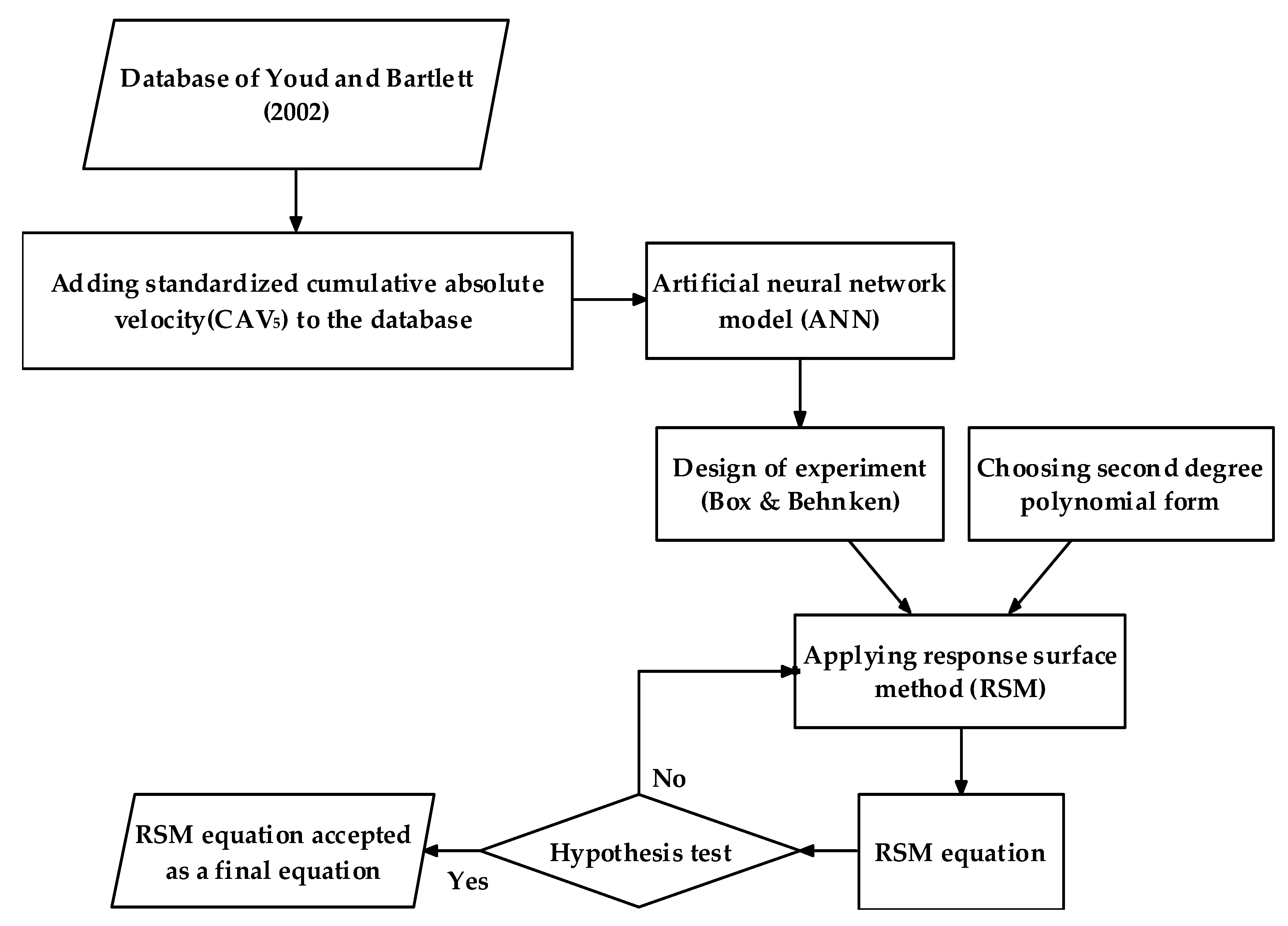
This study is based on the database of Youd et al. [20] and the addition of a new earthquake parameter of CAV₅, which is CAV with a 5-cm/sec² threshold acceleration, through the attenuation equation presented by Kramer et al. [21]. By adding CAV₅, the dataset was expanded and became more capable of and efficient in considering aspects of earthquakes and geology site situations, such as earthquake motion frequency, near-fault effects and the causative fault type of an earthquake. The second dataset was created by eliminating samples with an average Fc in a liquefiable soil layer (F₁₅) less than 28%. The response surface method (RSM) is used for the first time as a novel method to develop two equations to predict lateral displacement due to liquefaction (D_H) in order to two created datasets herein. 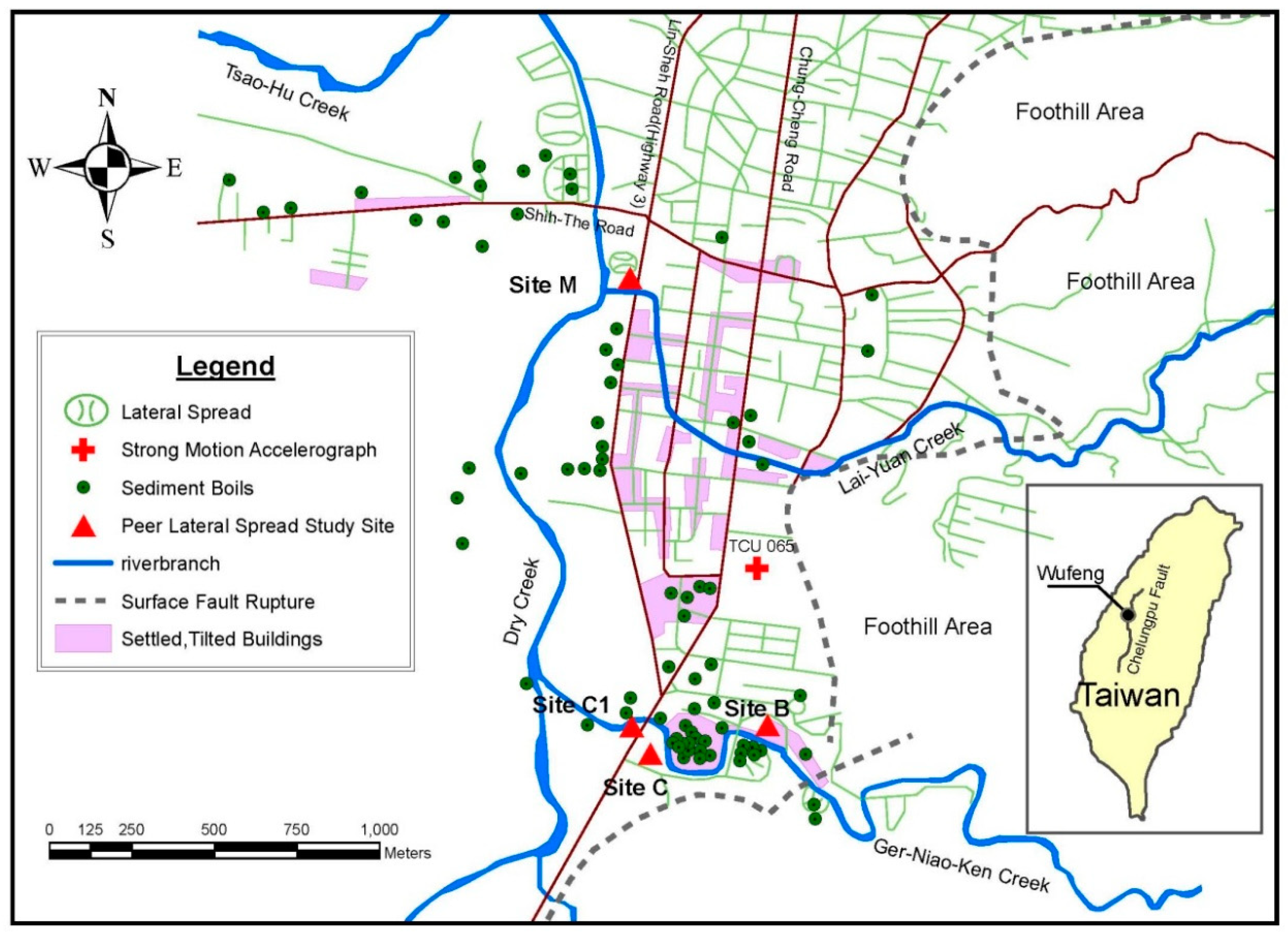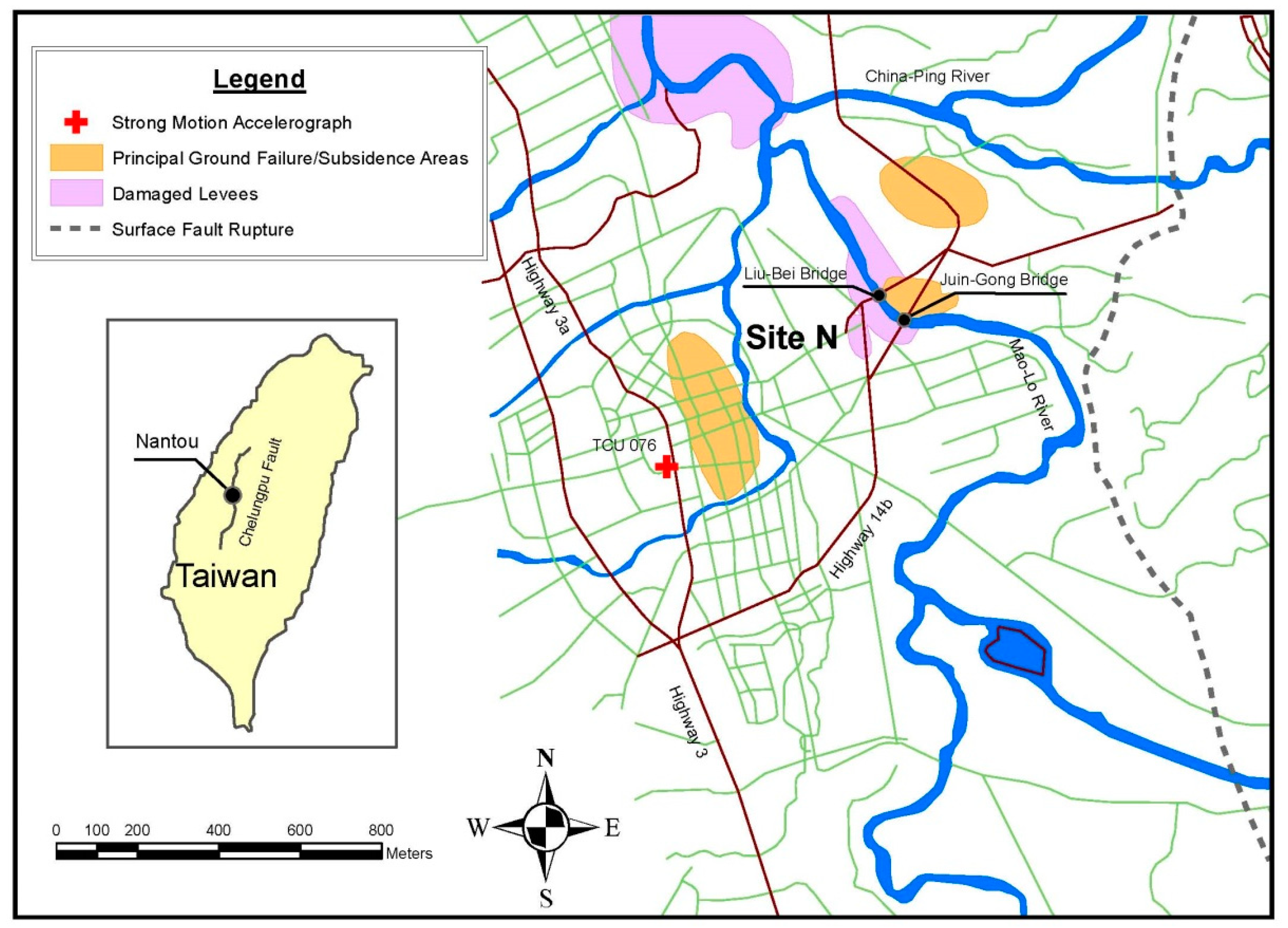Furthermore, the meaningful and effective terms of the equations are discovered through hypothesis testing of the p-value. In this study, two ANNs with back-propagation analysis were developed to measure the coding input data of the RSM. To develop each ANN model, the main dataset is first divided into three subsets for the training, testing, and validating stages, considering statistical properties—instead of random division—to increase the capability and accuracy of the model. To achieve this goal, an attempt is made to create all three subsets with close statistical factors. Finally, the results are compared with data measured from the Chi-Chi earthquake’s near fault zone of Wufeng district (Figure 1) and Nantou district (Figure 2), as well as with the predicted D_H through three extra models [20,27,36] to demonstrate the accuracy and capability of the RSM models.

2. Review of Empirical and Semi-Empirical Models

Bartlett and Youd [1], based on factors in References [13,14,29], developed a new model to predict D_H due to liquefaction; they supposed that earthquake, topographical, geological, and soil factors are the most influential parameters on D_H. They studied 467 displacement vectors from the case history database. Among those vectors, 337 were from the 1964 Niigata and 1983 Nihonkai-Chubu, Japan, earthquakes; 111 were from earthquakes in the United States; and the other 19 cases were selected from Ambraseys’ [29] database. In the end, they developed a new model by using multiple linear regression (MLR) for free-face and ground slope conditions [37], but they did not separate earthquakes according to their region because of a database shortage. Youd et al. revised their MLR by adding case history data from three earthquakes (1983 Borah Peak, Idaho; 1989 Loma Prieta; and 1995 Hyogoken-Nanbu (Kobe)), and they considered coarser-grained materials. They removed eight displacement sites with prevented free lateral movement and developed two equations with more accuracy given as follows:

Free-face conditions:

$$\log D_H=-16.713+1.532M-1.4\log r^{*}-0.012r+0.592\log W+0.540\log T_{15}+3.413\log \left(100-F_{15}\right)-0.795\log \left(D{50}_{15}+0.1 \mathrm{mm}\right)$$

(1)

Sloping ground conditions:

$$\log D_H=-16.213+1.532M_w-1.406\log r^{*}-0.012R+0.338\log S+0.540\log T_{15}+3.413\log \left(100-F_{15}\right)-0.795\log \left(D{50}_{15}+0.1 \mathrm{mm}\right)$$

(2)

where

$$r^{*}=r+r_0$$

(3)

and

$$r_0={10}^{\left(0.89M-5.64\right)}$$

(4)

In Equations (1) and (2), D_H is the predicted lateral ground displacement (m), M_w is the moment magnitude of the earthquake, and T₁₅ is the cumulative thickness of saturated granular layers (m) with corrected blow counts ((N₁)₆₀) less than 15. Moreover, F₁₅ is the average fines content of sediment within T₁₅ (%); D50₁₅ is the average mean grain size for granular materials within T₁₅ (mm); S is the ground slope (%); and W is the free-face ratio (H/L), where H is the height of the free face and L is the distance from the base of the free face to the liquefied point. Finally, r is the nearest horizontal or map distance from the site to the seismic energy source (Km).

Rezania et al. [37] developed a model, based on evolutionary polynomial regression, for the assessment of liquefaction potential and lateral spreading. According to response spectral acceleration, measured through strong-motion attenuation models, Zhang et al. [38] revised the empirical model of Youd et al. [20] and demonstrated the ability of their model by comparing the predicted results with datasets from sites in Turkey and New Zealand [18]. Goh et al. proposed multivariate adaptive regression splines (MARS) by using data of Youd et al. [20]. They demonstrated an improvement of the original model [39].

3. Artificial Neural Network

An ANN is a computational process using a biological neural network structure. McCulloch et al. [40] were the first to introduce some simulations according to their neurology knowledge. Neural networks are strong approximators due to their ability to learn by samples and their independency from any algorithm or knowledge about internal features of the issue. Artificial neural networks have a number of advantages such as high accuracy in nonlinear relationships or dynamic mechanisms based on the number and effectiveness of samples. Neural networks are classically constructed in three types of layers. Layers are provided by interconnected nodes. Outlines of the network are developed via the input layer, which communicates to one or more hidden layers by performing a weighting process. Then, hidden layers link to a target (output layer). Further, learning is a supervised process that occurs with each cycle or “epoch” (i.e., each time the network is presented with a new input pattern).

Rumelhart et al. [41] introduced a back-propagation algorithm to decrease error according to the training data. The training process started with random weights to achieve minimum error. The calculation of the derivatives flows backwards through the network, which is why it is called back-propagation. The most common measure of error is the MSE:

MSE = Ave {(actual output vector − desired output vector)²}

(5)

Overtraining of a neural network happens when the network trains exactly to reply to just one kind of input, which is similar to rote memorization. Therefore, learning does not occur anymore. The ANN is able to be used for problems with non-linear or dynamic correlation.

4. Response Surface Method

The RSM is a group of statistical and mathematical techniques to develop a capable function for a relationship of response (y) or output variable, and input variables (x), given by:

$$y=f^{\prime }\left(x\right)\beta +\epsilon$$

(6)

where f(x) is a vector function, consisting of powers and cross-products of input variables. This function depends on the supposed form of the response.

There are some common forms that have been used by researchers. A second-degree polynomial with cross terms is the most complicated and the strictest among them, and it is given by:

$$R_{\left(X\right)}=a_0+{\displaystyle \sum }_{i=1}^n{b}_i{X}_i+{\displaystyle \sum }_{i=1}^n{C}_i{X}_i{}^2+{\displaystyle \sum }_{\begin{array}{c}i=1\\ j\ne i\end{array}}^n{d}_{ij}{X}_i{X}_j$$

(7)

The main applications of RSM are defined as follows:

• To present an approximate relationship between input variables and an output variable or response to be able to predict the response variable.
• To discover significant factors or terms of the presented equation using RSM through hypothesis testing such as the p-value.
• To assess the optimization model to obtain a response as a maximum or minimum over a certain range of interest.

4.1. Design of Experiments

When more than one input factor is suspected of influencing an output, in order to fit physical or numerical experiments, a process by the name of design of experiments (DOE) [42] is developed. The DOE involves selecting some points according to which a response should be calculated.

In this paper, the design introduced by Box et al. [43] is used. It requires three levels to run an experiment. Furthermore, it is a special three-level design without any points at the vertices of the experiment region. This could be advantageous when the points on the corners of the cube represent level combinations that are prohibitively expensive or impossible to test because of physical process constraints. The design is applied in this study to prevent the input parameters’ values from being negative. This DOE requires three levels of each input variable −1, 0, 1 (coded values) corresponding to minimum, middle, and maximum values of input parameters, respectively.

4.2. Hypothesis Test

The process in statistics science to meaningfully examine results is called a hypothesis test. During hypothesis tests, the validity of a claim, which is constructed about a population, is evaluated. This claim that is in essence on trial is called the null hypothesis. Hypothesis testing can be expressed in three steps:

• Defining an initial assumption (null hypothesis).
• Analyzing and assessing sample data by following a formal process.
• Based on the second step, accepting or rejecting the initial assumption in the first step.

One of the main approaches to make a decision to accept or reject a null hypothesis is the p-value, defined through an α value (the probability of error is called alpha). If the p-value is smaller than α, then the null hypothesis is rejected, and contrarily, if it is larger, then the null hypothesis is accepted.

In this paper, the common value of 0.05, which researchers have used for α, is applied to analyze the meaningfulness and significance of parameters and the terms in the RSM response (equation).

5. Model Proposed

Figure 3 illustrates the flow chart of the applied approach to develop the RSM equations to estimate D_H in this study. Two models are presented: first one considered the whole range of the parameters and the second one was on the basis of the F₁₅ value being less than 18%.

5.1. Dataset

Bartlett et al. [37] collected 467 data samples of D_H from the following eight earthquakes in the United States and Japan: San Francisco 1906, Alaska 1964, Niigata 1964, San Fernando 1971, Imperial Valley 1979, Borah Peak 1983, Nihonkai-Chubu 1983, and Superstition Hills 1987. The parameters of the case histories that they collected to analyze were divided into three groups:

• Seismic parameters—moment magnitude (M_W) and horizontal distance from site to seismic energy source (r) in km.
• Topographic parameters—free-face ratio (W) and ground slope (S), both in percent.
• Geotechnical parameters—thickness of layer with corrected blow counts (N1)₆₀ < 15 (T₁₅) in meters, average fines content in the T₁₅ layer (F₁₅) in percent, and average mean grain size in the T₁₅ layer (D50₁₅) in mm.

Later, Youd et al. [20] eliminated eight sites’ data from their dataset due to a lack of free lateral movement. Additionally, they added data from the following three earthquake sites: Borah Peak 1983, Loma Prieta 1989, and Hyogo-Ken Nanbu (Kobe) 1995.

In the present study, the main dataset was developed by adding a new parameter of CAV₅, which is defined in Section 5.1.1. Kramer et al. [21] stated that CAV₅ is the most efficient and sufficient earthquake intensity to evaluate liquefaction in sandy soil. Therefore, CAV₅ was estimated using the attenuation equation presented by them.. In this way, the causative earthquake fault types of all earthquakes in the dataset were discovered. Then, the sites with a moment magnitude range from 6.4 to 7.9 were selected in order to find the applicable magnitude range for Equation (11); the Alaska 1964 site, with a magnitude of 9.2, was thus deleted from the dataset.

Furthermore, a statistical analysis was performed to examine and estimate the coefficient of correlation (R) of all input parameters with the output (D_H) one by one. The estimated values of R for r-D_H and S-D_H were a positive value of 0.104 and a negative value of −0.98, respectively, contrary to the supposition for them. This was possibly due to the scarcity of sites that were explored, and consequently, the shortage measured values for r and S in the main dataset. Therefore, in this study, after eliminating r and S from dataset, only the free-face condition was considered, and samples of the ground slope condition were deleted from the main dataset. Furthermore, CAV₅ was added to the dataset instead of r. Figure 4 and Figure 5 plot r versus CAV₅ for range of M_w in the main dataset from 6.4 to 7 and 7 to 7.9, respectively. It should be mentioned that the bold points show more than one point coincided together.

A dataset including 215 case histories with six parameters was then prepared. In addition, to investigate the complicated influence of fine content on the liquefaction, the second dataset was arranged by eliminating samples with an F₁₅ value larger than 28%. Therefore, the second dataset included 182 samples.

5.1.1. Cumulative Absolute Velocity

Eed et al. utilized CAV as a criterion to evaluate the onset of structural damage for the first time. They reported it in the Electric Power Research Institute journal [44] and defined it in a mathematical framework as presented below:

$$CAV={{\displaystyle \int }}_0^{t_{max}}\left|a\left(t\right)\right|dt$$

(8)

where a(t) is the acceleration of ground motion graph, t is the time, and t_max is the duration of the earthquake.

Liyanapathirana et al. [45] studied special aspects of Australian earthquakes and found that the predominant frequency of earthquakes in Australia is much higher than in California. This is because the earthquakes in Australia are in the middle of tectonic plates, so liquefaction has not occurred. They introduced a pseudo-velocity in the same dimensions and form as CAV to quantify this difference as indicated below:

$$V={{\displaystyle \int }}_0^{t_{max}}\left|a\left(t\right)\right|dt$$

(9)

By studying various Japanese codes, Orense demonstrated that seismic-induced shear stresses, calculated using empirical models containing PGA, do not have high accuracy in near-source circumstances but still have reasonable accuracy for far-source earthquakes. Next to that, he indicated threshold values of 150 gal and 20 kine for PGA and PGV respectively for the occurrence of liquefaction [46].

After inspecting approximately 300 parameters of earthquakes, Kramer et al. revealed that CAV₅, as can be estimated through Equation (11), has better efficiency and sufficiency than other earthquake intensity parameters for liquefaction evaluation. They also utilized the strong Pacific Earthquake Engineering Research (PEER) database, consisting of 282 ground motions from 40 earthquakes to present an equation to calculate CAV₅ for shallow crustal events [21].

$$CA{V}_5={{\displaystyle \int }}_0^{\infty }\langle ӽ\rangle \left|a\left(t\right)\right| where \langle ӽ\rangle =\{\begin{array}{c}0 for \left|a\left(t\right)\right|<5 \mathrm{cm}/\sec { }^2 \\ 1 for \left|a\left(t\right)\right|\ge 5 \mathrm{cm}/\sec {}^2 \end{array}$$

(10)

$$\ln CA{V}_5=3.495+2.764\left(M-6\right)+8.539\ln (M/6)+1.008\ln \left(\sqrt{r^2+6.155}\right)+{0.464}_1{F}_N+0.165F_R$$

(11)

where CAV₅ is a form of CAV based on Equation (10) (m/sec), M is the moment magnitude, and r is the closest distance to the rupture (km). F_N = F_R = 0 for strike slip faults, F_N = 1 and F_R = 0 for normal faults, and F_N = 0 and F_R = 1 for reverse or reverse-oblique faults.

The database of Equation (11) has a range of 4.7 to 7.4 for M, which is proposed for use for a maximum magnitude of 8, and it has a range of 1 to more than 100 km for r. In the present study, Equation (11) was applied to calculate CAV₅ from the dataset by considering the causative fault type.

5.2. Artificial Neural Network Models

At first, both datasets were divided into three groups: approximately 70% for the training phase and two groups of 15% each for the testing and validating phase. The validating phase was applied to prevent the model from being overtrained. The data deviation was conducted according to statistical factors, and the three groups contained similar statistical factors, such as minimum, maximum, and mean values. Furthermore, to achieve a higher accuracy of output, the same portion of any earthquake’s data was selected for the three phases, so all the sites contributed with their data in the training, testing, and validating phases with similar statistical factors. The ANN was established using a back-propagation algorithm with one hidden layer, which is the most commonly used network to drive an ANN model to predict D_H. There are six inputs, including six parameters, which were considered by Youd et al. [20] and Bartlett et al. [37]. In addition, there is the new measured parameter of CAV₅ as well as one output as a D_H.

The first dataset was divided into three groups including 151 samples for training, 32 samples for testing, and an extra 32 samples for the validating phase.

Table 1. Characteristics of whole case histories’ input parameters that were used to develop the ANN model and RSM equation.

Parameter	Min Value	Mean Value	Max Value
Mw	6.4	7.18	7.9
W (%)	1.64	10.25	56.8
T15 (m)	0.2	8.78	16.7
F15 (%)	1	16.57	70
D5015 (mm)	0.036	0.35	1.98
CAV5 (m/sec)	3.7	14.58	27.85

and

Table 2. Certificates of the first ANN model for the whole dataset.

Data	Training	Testing	Validating	All
R	0.89	0.92	0.90	0.90

summarize the characteristics and certificates of the first dataset and the subsequently developed ANN model. As can be seen from Table 2, the coefficient of correlation (R) given in Equation (12), which is the most common factor to assess the performance of correlations, of the first ANN model for all three groups and the main dataset was around 90%.

$$R=\frac{{{\displaystyle \sum }}_{i=1}^N\left(x_i-x_0\right)\left(d_i-d_0\right)}{\sqrt{{{\displaystyle \sum }}_{i=1}^N{(x_i-x_0)}^2{{\displaystyle \sum }}_{i=1}^N{(d_i-d_0)}^2}}$$

(12)

where n is the sample size, x_i and d_i are the individual sample points indexed with i, and $\overline{x}$ and $\overline{d}$ are the mean sample sizes.

To investigate the complex influence of F₁₅, the new dataset was constructed by selecting data samples with an F₁₅ less than critical value of 28%, which was demonstrated by Tao [32], and its characteristics are listed in

Table 3. Characteristics of database with F₁₅ ≤ 28% used for the second developed ANN model and RSM equation.

Parameter	Min Value	Mean Value	Max Value
Mw	6.5	7.27	7.9
W (%)	1.64	9.84	56.8
T15 (m)	0.5	8.78	16.7
F15 (%)	1	11.83	27
D5015 (mm)	0.086	0.4	1.98
CAV5 (m/sec)	3.7	15.02	16.28

. The new dataset was divided again into three groups with the same portion of each site and with similar statistical factors. Therefore, data from each earthquake contributed to the training, testing, and validating phase. In this step, around 15%, 15%, and 70% of the dataset equated to 27, 27, and 129 samples used for the testing, validating, and training processes, respectively. The characteristics of this new ANN model are presented in Table 3. Also,

Table 4. Certificate of the second ANN model for dataset with F₁₅ ≤ 28%.

Data	Training	Testing	Validating	All
R	0.92	0.95	0.89	0.91

presents the certificate of the second model. It can be seen in Table 4 that the R values for all groups of datasets were around 90%.

5.3. The RSM Equations for Predicting D_H

First, an RSM was conducted to drive an equation on the basis of the first ANN model. Therefore, the DOE introduced by Box et al. [43] for the second-degree polynomial with cross terms was employed to provide 54 coded values to cover the full range of parameters. Through the first developed ANN model, the response value (herein referred to as D_H) in coded form was calculated. Thereafter, the RSM equation with 28 terms according to the second-degree polynomial with cross terms was derived; however, through hypothesis testing considering the p-value, some terms were eliminated. Then, the RSM was applied repeatedly to achieve the final equation. The following equation was consequently developed with 22 terms to correlate the D_H caused by liquefaction to the six input parameters for the whole range of parameters in this study, without any limitations on the range of the F₁₅ value:

D_H = a₀ + a₁M_w + a₂W + a₃T₁₅ + a₄F₁₅ + a₅(D50₁₅) + a₆(CAV₅) + a₇M_w² + a₈W² + a₉T₁₅² + a₁₀(F₁₅)² + a₁₁(D50₁₅)² + a₁₂(CAV₅)² + a₁₃M_wT₁₅ + a₁₄M_wF₁₅ + a₁₅M_w(D50₁₅) + a₁₆WT₁₅ + a₁₇WF₁₅ + a₁₈W(D50₁₅) + a₁₉ T₁₅ F₁₅ + a₂₀ T₁₅ D50₁₅ + a₂₁ F₁₅ CAV₅

(13)

Characteristics of the RSM equation: R² = 87.22%, R² (predicted) = 78.73%, and R² (adjust) = 83.99%.

The coefficient of determination (R²) illustrates how well the curves fit on the data points. In addition, the R² (adjust) demonstrates the percentage of variation defined by the independent variables that affect the dependent variable, herein referred to as D_H. Also, the R² (predicted) defines how well a correlation is able to predict the target for a new observation. The values of coefficients a₀ to a₂₁ are listed in

Table 5. Coefficients of Equation (13).

Coefficient	a0	a1	a2	a3	a4	a5	a6	a7
Value	0.9174	−1.6737	2.6172	0.7685	−1.0865	−1.8952	1.3425	−0.36369
Coefficient	a8	a9	a10	a11	a12	a13	a14	a15
Value	−0.3733	−0.0678	−0.7474	−0.4060	0.0258	−0.3766	0.2579	−0.59428
Coefficient	a16	a17	a18	a19	a20	a21
Value	0.3566	−0.4549	0.4603	−0.6531	0.6011	−0.5063

.

Second, the second RSM equation with the final 21 terms was derived based on the second developed ANN model in this study through the same process as that for the first RSM equation. The second-degree polynomial with cross terms was applied in conjunction with Box and Behnken’s DOE on the basis of the second ANN model. Then, a hypothesis test with the same p-value was conducted to provide the second RSM equation for F₁₅ less than 28% (Equation (14)).

Table 6. Coefficients of Equation (14).

Coefficient	a0	a1	a2	a3	a4	a5	a6	a7
Value	3.1271	1.1700	0.4711	−0.02313	−0.6786	0.7715	−0.0208	0.5489
Coefficient	a8	a9	a10	a11	a12	a13	a14	a15
Value	−0.0871	−0.6520	0.3773	0.3225	−0.4646	0.6225	−0.7350	−0.7364
Coefficient	a16	a17	a18	a19	a20
Value	−0.7855	0.9542	0.9622	−0.8165	−1.2668

presents the coefficients of the second RSM equation.:

D_H = a₀ + a₁M_w + a₂W + a₃T₁₅ + a₄F₁₅ + a₅(D50₁₅) + a₆(CAV₅) + a₇M_w² + a₈W² + a₉T₁₅² + a₁₀(F₁₅)² + a₁₁(D50₁₅)² + a₁₂(CAV₅)² + a₁₃M_wW + a₁₄M_wF₁₅ + a₁₅M_w(CAV₅) + a₁₆W(D50₁₅) + a₁₇W(CAV₅) + a₁₈ T₁₅ F₁₅ + a₁₉ T₁₅ (D50₁₅) + a₂₀ F₁₅ (D50₁₅)

(14)

Characteristics of the second RSM equation: R² = 88.51%, R² (predicted) = 50.95%, and R² (adjust) = 78.09%.

It must be noted that to use the derived RSM equation, the main values of input parameters must be exchanged with coded values by the function presented in Equation (15). Those coded values must then be put into the RSM equation to achieve the results. In other words, the RSM equation declares the relationship between the coded value of parameters and responses (output); coded values have a range from −1 to 1.

$$Coded value=\frac{Real value-mean value }{Max value-Min value}\times 2$$

(15)

The max, min, and mean values of the parameters are listed in Table 1 and Table 3 for both RSM equations presented in this study.

6. Comparison of RSM Equations with Extra Models

Chu et al. [47] analyzed five liquefied sites during the Chi-Chi-1999 earthquake in Taiwan, all in the near-fault region from five sites in two districts of Wufeng and Natu as they are illustrated in Figure 1 and Figure 2.

Table 7. Model parameters and measured D_H at sites affected by the 1999 Chi-Chi earthquake.

Sample No	Mw	r	W	S	T15	F15	D5015	PGA	CAV5	DH (m)
1	7.6	5	7.4	0	0.5	20.8	0.11	0.67	45.226	0
2	7.6	5	13.7	0	0.8	20.8	0.11	0.67	45.226	0.45
3	7.6	5	18.4	0	0.8	20.8	0.11	0.67	45.226	0.55
4	7.6	5	25.2	0	0.8	20.8	0.11	0.67	45.226	0.8
5	7.6	5	37.3	0	0.8	20.8	0.11	0.67	45.226	1.05
6	7.6	5	49.9	0	0.8	20.8	0.11	0.67	45.226	2.05
7	7.6	5	5.7	0	0.5	13	0.18	0.67	45.226	0
8	7.6	5	6.6	0	0.75	13	0.18	0.67	45.226	0.1
9	7.6	5	7.9	0	0.75	13	0.18	0.67	45.226	0.17
10	7.6	5	9	0	0.75	13	0.18	0.67	45.226	0.23
11	7.6	5	15	0	0.75	13	0.18	0.67	45.226	0.29
12	7.6	5	21.2	0	0.75	13	0.18	0.67	45.226	0.49
13	7.6	5	11.9	0	1.1	20.8	0.11	0.67	45.226	0
14	7.6	5	26.3	0	1.1	20.8	0.11	0.67	45.226	0
15	7.6	5	12.2	0	0.45	30	0.13	0.67	45.226	0.4
16	7.6	5	14.3	0	0.45	30	0.13	0.67	45.226	0.65
17	7.6	5	24.6	0	0.45	30	0.13	0.67	45.226	1
18	7.6	5	57.7	0	0.45	30	0.13	0.67	45.226	1.24
19	7.6	5	8	0	1	31.4	0.1	0.67	45.226	0.35
20	7.6	5	10.5	0	1	31.4	0.1	0.67	45.226	0.61
21	7.6	5	19	0	1	31.4	0.1	0.67	45.226	0.96
22	7.6	5	31.3	0	1	31.4	0.1	0.67	45.226	2.96
23	7.6	5	9.6	0	1.8	48.5	0.1	0.67	45.226	0.35
24	7.6	5	11.7	0	1.8	48.5	0.1	0.67	45.226	0.52
25	7.6	5	13.3	0	1.8	48.5	0.1	0.67	45.226	0.62
26	7.6	5	23.7	0	1.8	48.5	0.1	0.67	45.226	1.62
27	7.6	13	5.9	3.8	1.7	22.3	0.12	0.39	24.816	0.05
28	7.6	13	16.2	3.8	1.7	22.3	0.12	0.39	24.816	0.25

presents these parameters’ values from the sites. Based on these data samples, the predicted results of the RSM equations are compared to Youd et al. [20], Javadi et al. [27], and Rezania et al. [36]. In total, 28 sites (for which the necessary parameters for the ANN model and the RSM equation are reported by Chu et al. [45]) are illustrated in

Table 8. Performance certificate of first RSM equation in comparison with extra available models.

Performance Criteria	Models Used to Predict DH
	Youd et al. [20]	Javadi et al. [26]	Rezania et al. [36]	First RSM
R	0.514	−0.74	0.433	0.683
MAE	3.77	1.04	0.49	0.3
RSME	4.37	1.19	0.7	0.37

. The sample numbers from 1 to 26 are from Wufeng’s sites and samples of 27 and 28 are belong to Nantu’s site. The capability and accuracy of the first RSM equation was demonstrated using all 28 site samples from the Chi-Chi earthquake, including samples with F₁₅ from 13% to 48.5%.

The results of comparison between the predicted values and measured values are summarized in terms of the root mean square error (RMSE), mean absolute error (MAE), and R in Table 8. It is clear that the larger R and smaller RMSE and MAE reveal higher accuracy of predicted results.

$$RSME=\sqrt{\frac{{{\displaystyle \sum }}_N{(X_m-X_P)}^2}{N}}$$

(16)

$$MAE=\frac{{{\displaystyle \sum }}_N\left|X_m-X_P\right|}{N}$$

(17)

where N is the number of samples, X_m is the measured value, and X_P is the predicted value.

Furthermore, all samples with an F₁₅ greater than 28% were eliminated from the Chi-Chi earthquake cases, and 16 samples consequently remained (samples number 1 to 14 as well as numbers 27 and 28, as can be seen in Table 7). Then, the second RSM equation was validated by applying it to these samples in comparison with the extra three models.

Table 9. Performance certificate of second RSM equation, on the basis of samples with F₁₅ ≤ 28% in comparison with extra available models.

Performance Criteria	Models Used to Predict DH
	Youd et al. [20]	Javadi et al. [26]	Rezania et al. [36]	First RSM	Second RSM
R	0.934	−0.813	0.233	0.846	0.891
MAE	4.84	1.2	0.42	1.48	0.29
RSME	5.34	1.3	0.57	1.63	0.39

summarizes the results of all models.

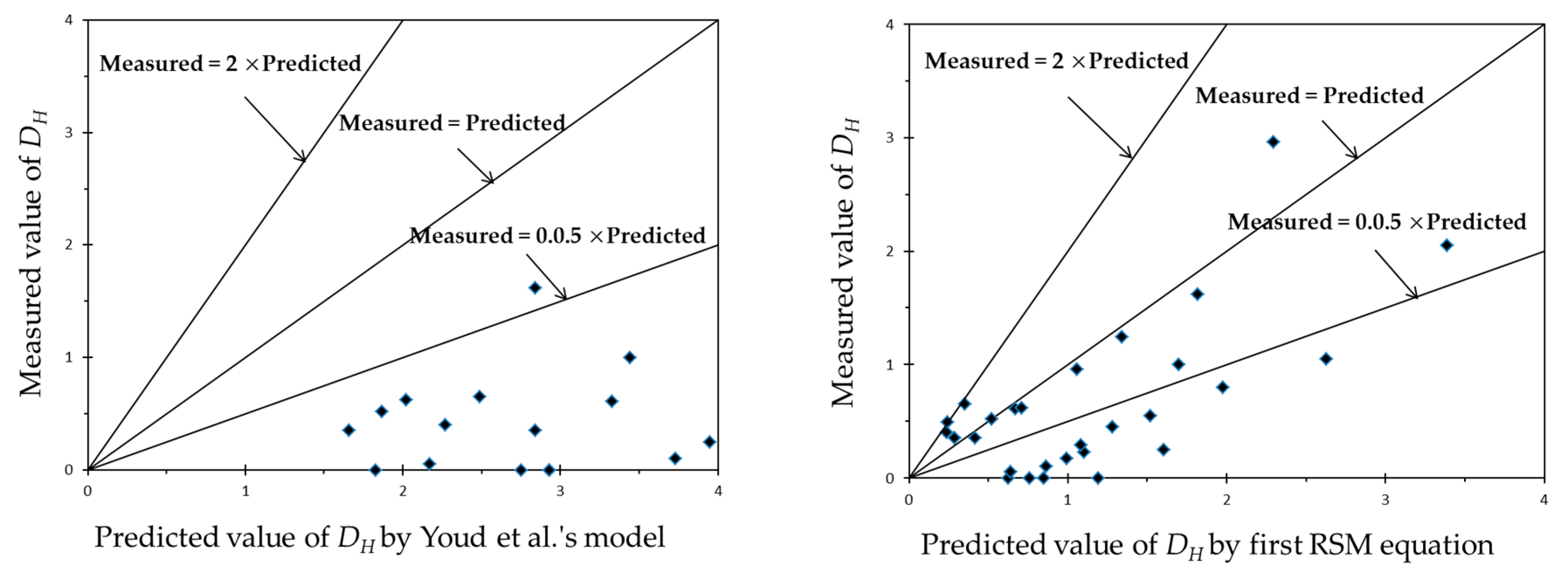
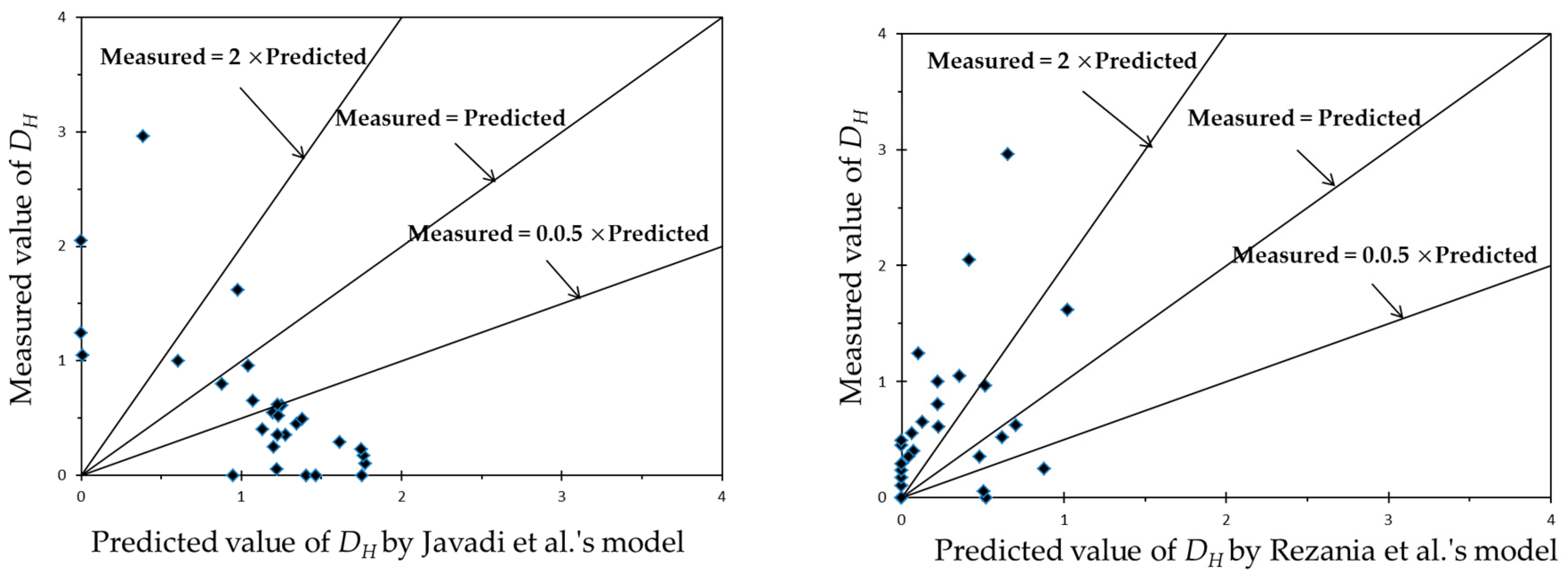
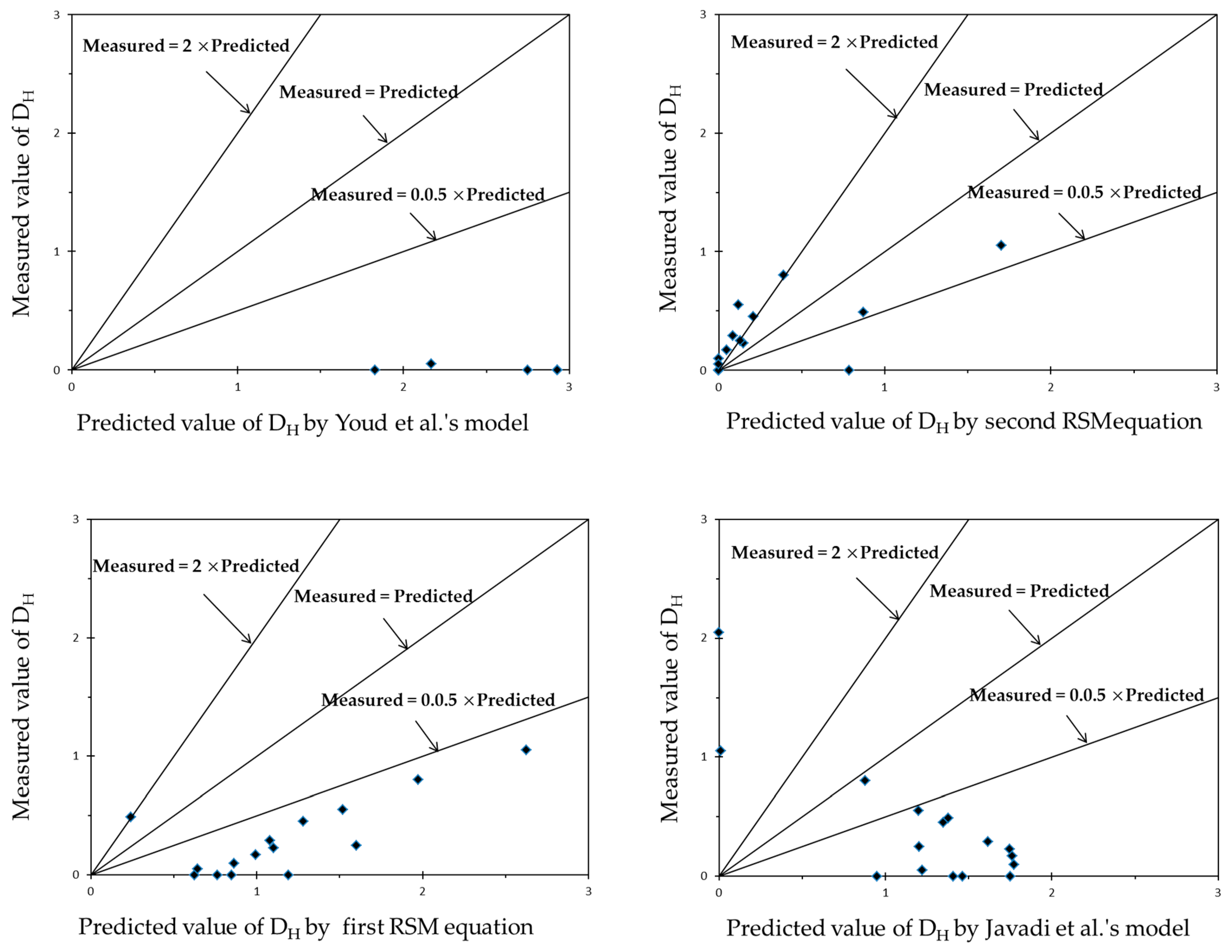
Figure 6 and Figure 7 visualize the comparison between both RSM equations developed in the present study and three extra models with measured data from sites of the Chi-Chi earthquake. Twenty-eight data points are evaluated in Figure 6 for whole range of the parameters. Meanwhile, Figure 7 illustrates the comparison for data points with F₁₅ values of less than 28% at 16 data points.

7. Results and Discussion

The previous sections have compared the first RSM model, which belongs to the full range of parameters, and the second RSM model, which was derived for samples whose F₁₅ values were less than 28%, with three extra well-known models. The models were examined using new data from the Chi-Chi earthquake, which were not included in the two datasets to establish the two RSM models. As can be seen in Table 8, the RSM equation of the whole range of parameters indicated a higher R value of 0.683, in comparison with the extra models whose values were 0.433, −0.74, and 0.514. Furthermore, the RSM model comprises lower MAE and RSME values of 0.3 and 0.37, respectively, compared to 0.49 and 0.7 for Rezania et al., 1.04 and 1.19 for Javadi et al., and 3.77 and 4.37 for Youd et al. Therefore, among all of them, the RSM model provided prediction with higher accuracy.

On the other hand, as can be seen in Table 9, by considering samples with F₁₅ less than 28%, the model of Youd et al. provided the highest R value of 0.934, closely followed by the second and the first RSM models with R values equal to 0.891 and 0.846 respectively. Table 9 also illustrates the MAE and RSME criteria values for all models for samples with a limited value for F₁₅ less than 28%. The values of the MAE and RSME in the second RSM model—0.29 and 0.39, respectively—indicates the highest accuracy and performance in comparison with the others. In addition, the model of Rezania et al., with 0.42 and 0.57, illustrated lower values for the MAE and RSME, respectively. Further, Javadi et al. with 1.2 and 1.3, and Youd et al. with 4.84 and 5.34 provide less accuracy for predicting D_H.

The comparison between the two models developed in this study and the extra three models demonstrates that the second RSM model provided a reasonable correlation and the lowest error. The results indicated that the RSM is a highly efficient tool to perform a liquefaction hazard analysis. Furthermore, performance of the model is increased by taking into account the complex influence of Fc by eliminating an F₁₅ larger than 28% and even by decreasing the number of samples in the dataset.

Another major advantage of the presented models is their consideration of earthquake aspects, such as the near-fault zone, the frequency of earthquake motion, and the causative fault type, by estimating and adding the CAV₅ parameter to the dataset. As can be seen from Figure 6 and Figure 7, among all models that were considered in the present study to calculate D_H without any limitation on the parameters’ value, the model of Youd et al. was overpredicted. Meanwhile, Youd et al.’s model provided poor and overpredicted results for samples with a limited value of F₁₅ less than 28%. Additionally, considering samples with a limited F₁₅ value shows the first RSM and the model of Javadi et al. present an overpredicted value for D_H. Furthermore, second RSM equation and model of Rezania et al. underpredicted D_H in their predictions.

There are some limitations for applying both first and second RSM equations as follow:

(1)

Both RSM models require standard penetration test SPT and laboratory tests to determine geotechnical properties parameters of T₁₅, F₁₅, and D50_15.

(2)

Both of the RSM models are valid for free-face conditions but not ground-slope conditions.

(3)

Second RSM model is valid only for F₁₅ < 28%.

(4)

Models are only valid for earthquakes with M_w between 6.4 and 8.0.

(5)

Specify accuracy limits for each model.

(6)

It is necessary to transfer all six input models’ parameters measured value to a coded value using Equation (15) and then put the coded value in the RSM equations to predict D_H.

8. Summary and Conclusions

The determination of lateral displacement due to liquefaction caused by an earthquake (D_H) is the most important aspect of liquefaction hazard analysis. There are two main types of conditions according to the topography of the sites: free-face and sloping ground conditions. 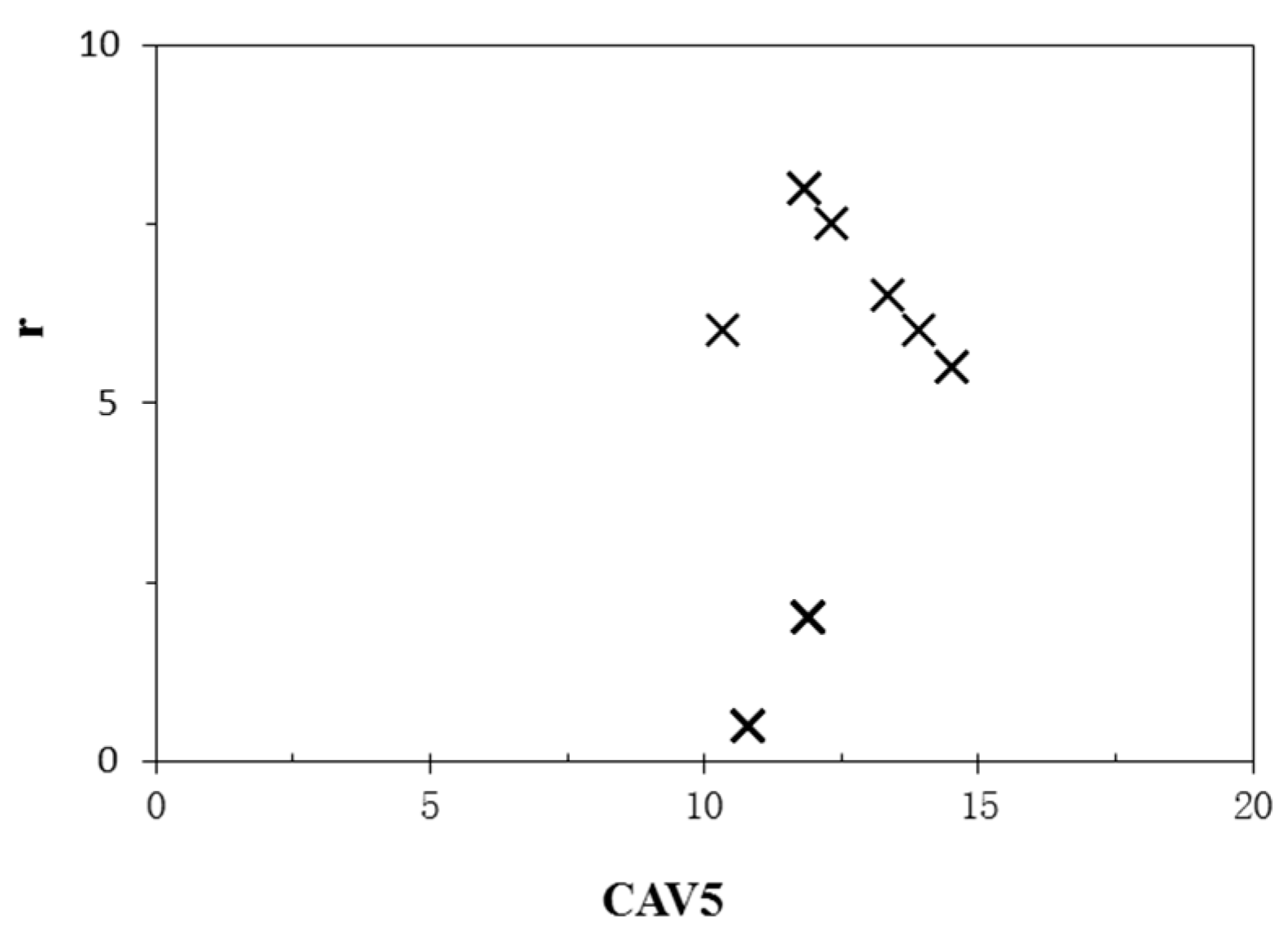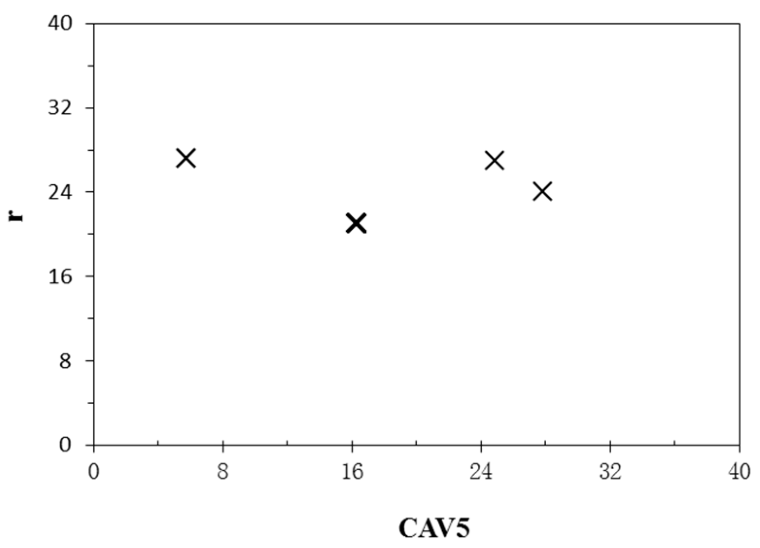First, the parameter of corrected absolute velocity (CAV₅) of sites was calculated due to it being the most efficient and sufficient parameter for the assessment of liquefaction caused by earthquakes [21], and it was added to develop the dataset to cover all aspects of earthquakes, including the frequency content of earthquake motions and the causative fault type of earthquakes. Then, a statistical parametric analysis was performed by estimating the correlation coefficient (R) between all input parameters and output as D_H. To achieve a more capable and accurate model, based on the estimated values for R, the horizontal distance from a site to the seismic energy source (r) and ground slope (S) was eliminated from the original dataset due to poor correlations to the target. Therefore, the final dataset was created for free-face condition sites.

The significant aspects of earthquakes, such as the near-fault region, frequency content, and causative fault type of earthquakes, which are included in the model established by Kramer et al. [21], were considered by taking CAV₅ into account. To investigate the complex effect of fine content, the main dataset was divided into two subsets. The first dataset included the whole range of parameters, and in the second one, all samples with average fine content in the liquefiable layer (F₁₅) larger than 28% were removed from the dataset, in line with Tao [32]. Furthermore, the RSM was applied to develop two equations in order to the first and the second dataset to examine its performance to assess liquefaction. In the end, the two presented models in this study were compared to three available models to demonstrate their capability and accuracy with regard to predicting D_H in free-face conditions in a near fault zone case history of the Chi-Chi earthquake.

The present study highlights the importance of earthquake aspects, especially CAV₅ as the most sufficient and efficient intensity to liquefaction hazard assessments. In addition, the RSM is a strong tool for the evaluation of complex non-linear phenomena such as liquefaction.

The results also confirm the complicated influence of F₁₅ on the whole range, and they provide significant enhancements to the performance of the model by considering samples with an F₁₅ less than 28% as a critical value defined by Tao [32]. One of the most remarkable results, which shows the complex influence of fine content on evaluation of D_H, is that the second model demonstrated higher accuracy and capability, even though it was developed using a database with fewer samples than the first model.

References

1. Bartlett, S.F.; Youd, T.L. Empirical Analysis of Horizontal Ground Displacement Generated by Liquefaction-Induced Lateral Spread; Tech. Rep. No. NCEER-92-0021; National Center for Earthquake Engineering Research: Buffalo, NY, USA, 1992; p. 114. [Google Scholar]
2. Gu, W.H.; Morgenstern, N.R.; Robertson, P.K. Progressive Failure of Lower San Fernando Dam. J. Geotech. Eng. 1993, 119, 339–449. [Google Scholar] [CrossRef]
3. Arulanandan, K.; Li, X.S.; Sivathasan, K.S. Numerical Simulation of Liquefaction-Induced Deformations. J. Geotech. Geoenviron. Eng. 2000, 126, 657–666. [Google Scholar] [CrossRef]
4. Liao, T.; McGillivray, A.; Mayne, P.W.; Zavala, G.; Elhakim, A. Seismic Ground Deformation Modeling; Final Report for MAE HD-7a (Year 1); Geosystems Engineering/School of Civil & Environmental Engineering, Georgia Institute of Technology: Atlanta, GA, USA, 2002. [Google Scholar]
5. Liyanapathirana, D.S.; Poulos, H.G. A numerical model for dynamic soil liquefaction analysis. Soil Dyn. Earthq. Eng. 2002, 22, 1007–1015. [Google Scholar] [CrossRef]
6. Lopez-Caballero, F.; Farahmand-Razavi, A.M. Numerical simulation of liquefaction effects on seismic SSI. Soil Dyn. Earthq. Eng. 2008, 28, 85–98. [Google Scholar] [CrossRef]
7. Tokida, K.; Matsumoto, H.; Azuma, T.; Towhata, I. Simplified Procedure to Estimate Lateral Ground Flow by Soil Liquefaction; Soil Dynamic and Earthquake Engineering, VI; Cakmak, A.S., Brebbia, C.A., Eds.; Elsevier Applied Science: New York, NY, USA, 1993; pp. 381–396. [Google Scholar]
8. Yegian, M.K.; EMarciano, A.; Ghahraman, V.G. Earthquake-Induced Permanent Deformations: Probabilistic Approach. J. Geotech. Eng. 1991, 117, 35–50. [Google Scholar] [CrossRef]
9. Baziar, M.H.; Dobry, R.; Elgamal, A.-W. Engineering Evaluation of Permanent Ground Deformation due to Seismically-Induced Liquefaction; Technical Report No. NCEER-92-0007; National Center for Earthquake Engineering Research, State University of New York: Buffalo, NY, USA, 1992; Volume 2. [Google Scholar]
10. Jibson, R.W. Predicting Earthquake-Induced Landslide Displacement Using Newmark–s Sliding Block Analysis; Transportation Research Record 1411; Transportation Research Board: Washington, DC, USA, 1994; pp. 9–17. [Google Scholar]
11. Miller, E.A.; Roycrof, G.A. Seismic Performance and Deformation of Leeves: Four case studies. J. Geotech. Geoenviron. Eng. 2004, 130, 344–354. [Google Scholar] [CrossRef]
12. Olson, S.M.; Johnson, C.I. Analyzing Liquefaction-Induced Lateral Spreads Using Strength Ratios. J. Geotech. Geoenviron. Eng. 2008, 134, 1035–1049. [Google Scholar] [CrossRef]
13. Hamada, M.; Towhata, I.; Yasuda, S.; Isoyama, R. Study on permanent ground displacement induced by seismic liquefaction. Comput. Geotech. 1987, 4, 197–220. [Google Scholar] [CrossRef]
14. Youd, T.L.; Perkins, D.M. Mapping of Liquefaction Severity Index. J. Geotech. Eng. 1987, 113, 1374–1392. [Google Scholar] [CrossRef]
15. Shamoto, Y.; Zhang, J.-M.; Tokimatsu, K. Methods for evaluating residual post-liquefaction ground settlement and horizontal displacement. Soils Found. 1998, 38, 69–83. [Google Scholar] [CrossRef]
16. Kanıbir, A.; Ulusay, R.; Aydan, Ö. Assessment of liquefaction and lateral spreading on the shore of Lake Sapanca during the Kocaeli (Turkey) earthquake. Eng. Geol. 2006, 83, 307–331. [Google Scholar] [CrossRef]
17. Franke, K.W.; Kramer, S.L. Procedure for the Empirical Evaluation of Lateral Spread Displacement Hazard Curves. J. Geotech. Geoenviron. Eng. 2014, 140, 110–120. [Google Scholar] [CrossRef]
18. Zhang, J.; Zhao, J.X. Empirical models for estimating liquefaction-induced lateral spread displacement. Soil Dyn. Earthq. Eng. 2005, 25, 439–450. [Google Scholar] [CrossRef]
19. Bardet, J.-P.; Liu, F. Motions of gently sloping ground during earthquakes. J. Geophys. Res. Earth Surf. 2009, 114. [Google Scholar] [CrossRef]
20. Youd, T.L.; Hansen, C.M.; Bartlett, S.F. Revised Multilinear Regression Equations for Prediction of Lateral Spread Displacement. J. Geotech. Geoenviron. Eng. 2002, 128, 1007–1017. [Google Scholar] [CrossRef]
21. Kramer, S.L.; Mitchell, R.A. Ground Motion Intensity Measures for Liquefaction Hazard Evaluation. Earthq. Spectra 2006, 22, 413–438. [Google Scholar] [CrossRef]
22. Shome, N. Probabilistic Seismic Demand Analysis of Nonlinear Structures; Stanford University: Stanford, CA, USA, 1999; p. 320. [Google Scholar]
23. Hui, S.; Tang, L.; Zhang, X.; Wang, Y.; Ling, X.; Xu, B. An investigation of the influence of near-fault ground motion parameters on the pile’s response in liquefiable soil. Earthq. Eng. Eng. Vib. 2018, 17, 729–745. [Google Scholar] [CrossRef]
24. Kwan, W.S.; Sideras, S.S.; Mohtar, C.E. Predicting Soil Liquefaction Lateral Spreading: The Missing Time Dimension. In Proceedings of the Geotechnical Earthquake Engineering and Soil Dynamics V, Austin, TX, USA, 10–13 June 2018. [Google Scholar]
25. Wang, J.; Rahman, M.S. A neural network model for liquefaction-induced horizontal ground displacement. Soil Dyn. Earthq. Eng. 1999, 18, 555–568. [Google Scholar] [CrossRef]
26. Baziar, M.H.; Ghorbani, A. Evaluation of lateral spreading using artificial neural networks. Soil Dyn. Earthq. Eng. 2005, 25, 1–9. [Google Scholar] [CrossRef]
27. Javadi, A.A.; Rezania, M.; Nezhad, M.M. Evaluation of liquefaction induced lateral displacements using genetic programming. Comput. Geotech. 2006, 33, 222–233. [Google Scholar] [CrossRef]
28. Baziar, M.H.; Saeedi Azizkandi, A. Evaluation of lateral spreading utilizing artificial neural network and genetic programming. Int. J. Civ. Eng. 2013, 11, 100–111. [Google Scholar]
29. Ambraseys, N.N.; Menu, J.M. Earthquake-induced ground displacements. Earthq. Eng. Struct. Dyn. 1988, 16, 985–1006. [Google Scholar] [CrossRef]
30. Derakhshandi, M.; Rathje, E.M.; Hazirbaba, K.; Mirhosseini, S.M. The effect of plastic fines on the pore pressure generation characteristics of saturated sands. Soil Dyn. Earthq. Eng. 2008, 28, 376–386. [Google Scholar] [CrossRef]
31. Phan, V.T.-A.; Hsiao, D.-H.; Nguyen, P.T.-L. Effects of Fines Contents on Engineering Properties of Sand-Fines Mixtures. Procedia Eng. 2016, 142, 213–220. [Google Scholar] [CrossRef]
32. Tao, M. Case History Verification of the Energy Method to Determine the Liquefaction Potential of Soil Deposits; Department of Civil Engineering, Case Western Reserve University: Cleveland, OH, USA, 2003; p. 173. [Google Scholar]
33. Youd, T.L. Application of MLR Procedure for Prediction of Liquefaction-Induced Lateral Spread Displacement. J. Geotech. Geoenviron. Eng. 2018, 144, 04018033. [Google Scholar] [CrossRef]
34. Pirhadi, N.; Tang, X.; Yang, Q.; Kang, F. A New Equation to Evaluate Liquefaction Triggering Using the Response Surface Method and Parametric Sensitivity Analysis. Sustainability 2018, 11, 112. [Google Scholar] [CrossRef]
35. Maurer, B.W.; Green, R.A.; Cubrinovski, M.; Bradley, B.A. Fines-content effects on liquefaction hazard evaluation for infrastructure in Christchurch, New Zealand. Soil Dyn. Earthq. Eng. 2015, 76, 58–68. [Google Scholar] [CrossRef]
36. Rezania, M.; Faramarzi, A.; Javadi, A.A. An evolutionary based approach for assessment of earthquake-induced soil liquefaction and lateral displacement. Eng. Appl. Artif. Intell. 2011, 24, 142–153. [Google Scholar] [CrossRef]
37. Bartlett, S.F.; Youd, T.L. Empirical Prediction of Liquefaction-Induced Lateral Spread. J. Geotech. Eng. 1995, 121, 316–329. [Google Scholar] [CrossRef]
38. Zhang, G.; Robertson, P.K.; Brachman, R.W.I. Estimating Liquefaction-Induced Lateral Displacements Using the Standard Penetration Test or Cone Penetration Test. J. Geotech. Geoenviron. Eng. 2004, 130, 861–871. [Google Scholar] [CrossRef]
39. Goh, A.T.C.; Zhang, W.G. An improvement to MLR model for predicting liquefaction-induced lateral spread using multivariate adaptive regression splines. Eng. Geol. 2014, 170, 1–10. [Google Scholar] [CrossRef]
40. McCulloch, W.S.; Pitts, W. A logical calculus of the ideas immanent in nervous activity. Bull. Math. Biophys. 1943, 5, 115–133. [Google Scholar] [CrossRef]
41. Rumelhart, D.E.; McClelland, J.L. Parallel Distributed Processing; MIT Press: Cambridge, MA, USA, 1986. [Google Scholar]
42. Box, G.E.P.; Draper, N.R. Empirical Model-Building and Response Surfaces; John Wiley & Sons: New York, NY, USA, 1987. [Google Scholar]
43. Box, G.E.P.; Behnken, D.W. Some New Three Level Designs for the Study of Quantitative Variables. Technometrics 1960, 2, 455–475. [Google Scholar] [CrossRef]
44. EPRI. A Criterion for Determining Exceedance of the Operating Basis Earthquake; Report No. EPRI NP-5930; EPRI: Palo Alto, CA, USA, 1988; p. 330. [Google Scholar]
45. Liyanapathirana, D.S.; Poulos, H.G. Assessment of soil liquefaction incorporating earthquake characteristics. Soil Dyn. Earthq. Eng. 2004, 24, 867–875. [Google Scholar] [CrossRef]
46. Orense, R.P. Assessment of liquefaction potential based on peak ground motion parameters. Soil Dyn. Earthq. Eng. 2005, 25, 225–240. [Google Scholar] [CrossRef]
47. Chu, D.B.; Stewart, J.P.; Youd, T.L.; Chu, B.L. Liquefaction-Induced Lateral Spreading in Near-Fault Regions during the 1999 Chi-Chi, Taiwan Earthquake. J. Geotech. Geoenviron. Eng. 2006, 132, 1549–1565. [Google Scholar] [CrossRef]
Figure 1. Location of lateral displacement and ground failure due to liquefaction during the Chi-Chi earthquake in the Wufeng district.
Jmse 07 00035 g001
Figure 2. Location of lateral displacement and ground failure due to liquefaction during the Chi-Chi earthquake in the Nantou district.
Jmse 07 00035 g002
Figure 3. Flowchart of the approach applied in this study to present an equation to predict lateral displacement caused by liquefaction.
Jmse 07 00035 g003
Figure 4. r versus CAV5 for 6.4 ≤ Mw < 7 of the main dataset applied in this study.
Jmse 07 00035 g004
Figure 5. r versus CAV5 for 7 ≤ Mw ≤ 7.9 of the main dataset applied in this study.
Jmse 07 00035 g005
Figure 6. Comparison between the first RSM equation and three extra models with 28 data points measured from sites of Chi-Chi earthquake.
Jmse 07 00035 g006aJmse 07 00035 g006b
Figure 7. Comparison between both RSM equations and three extra models with 16 data points including F15 of less than 28% measured from sites of the Chi-Chi earthquake.
Jmse 07 00035 g007aJmse 07 00035 g007b