Impact Assessment of a Major River Basin in Bangladesh on Storm Surge Simulation

 ,
,
Abstract
:1. Introduction
2. Study Area and Cyclones
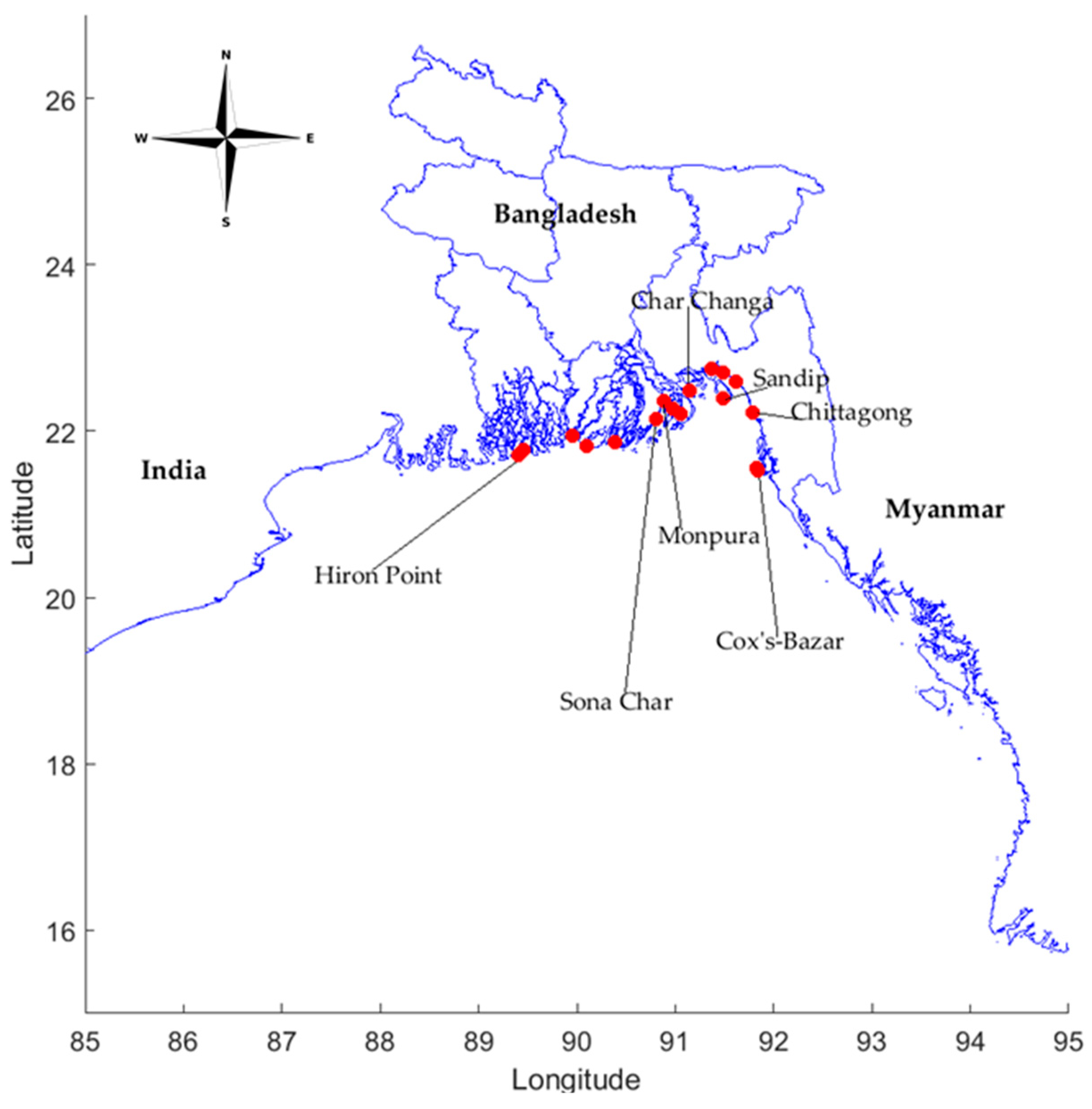
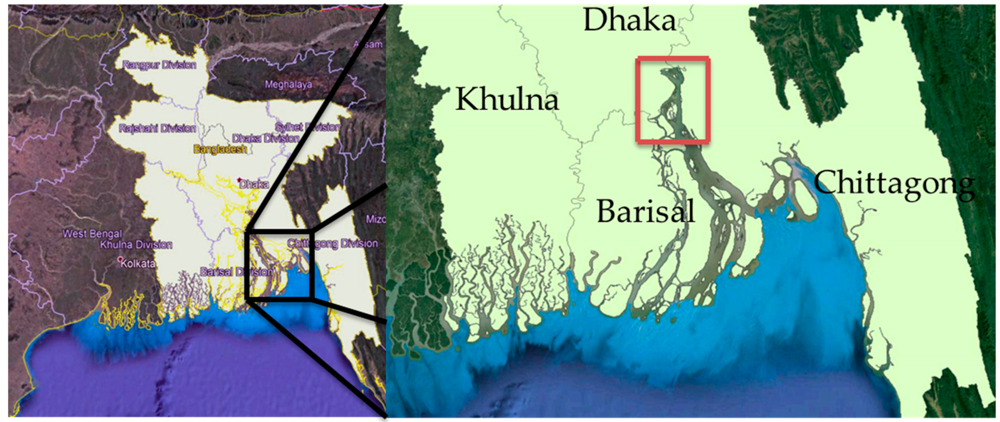
2.1. Study Area
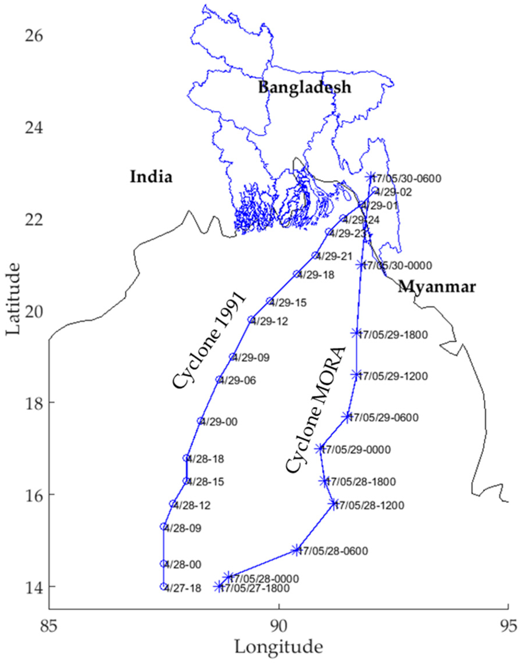
2.2. Cyclones
2.2.1. Cyclone 1991 (BoB 01)
2.2.2. Cyclone MORA
3. Numerical Model
3.1. Data and Materials
3.2. Model Description
3.2.1. Parent Model (Bay Model)
3.2.2. River Model
3.3. Boundary Conditions
3.3.1. Boundary Condition of the Parent Model
3.3.2. Boundary Condition for the River Model
3.3.3. Matching Boundary Condition
4. Numerical Procedure
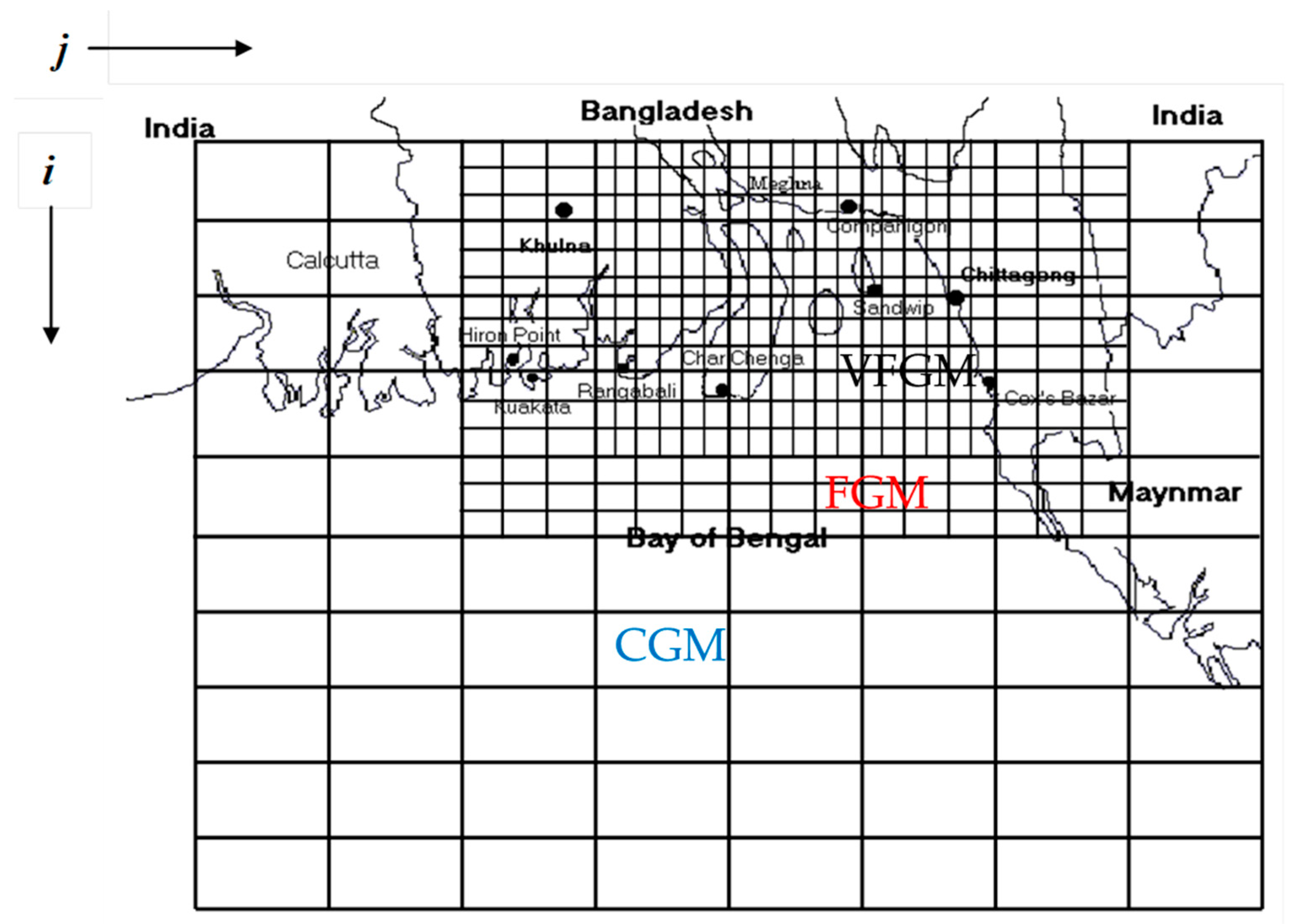
4.1. Nested Model Set Up
4.2. Numerical Procedure
4.3. Numerical Conditions
5. Model Validation and Outcomes
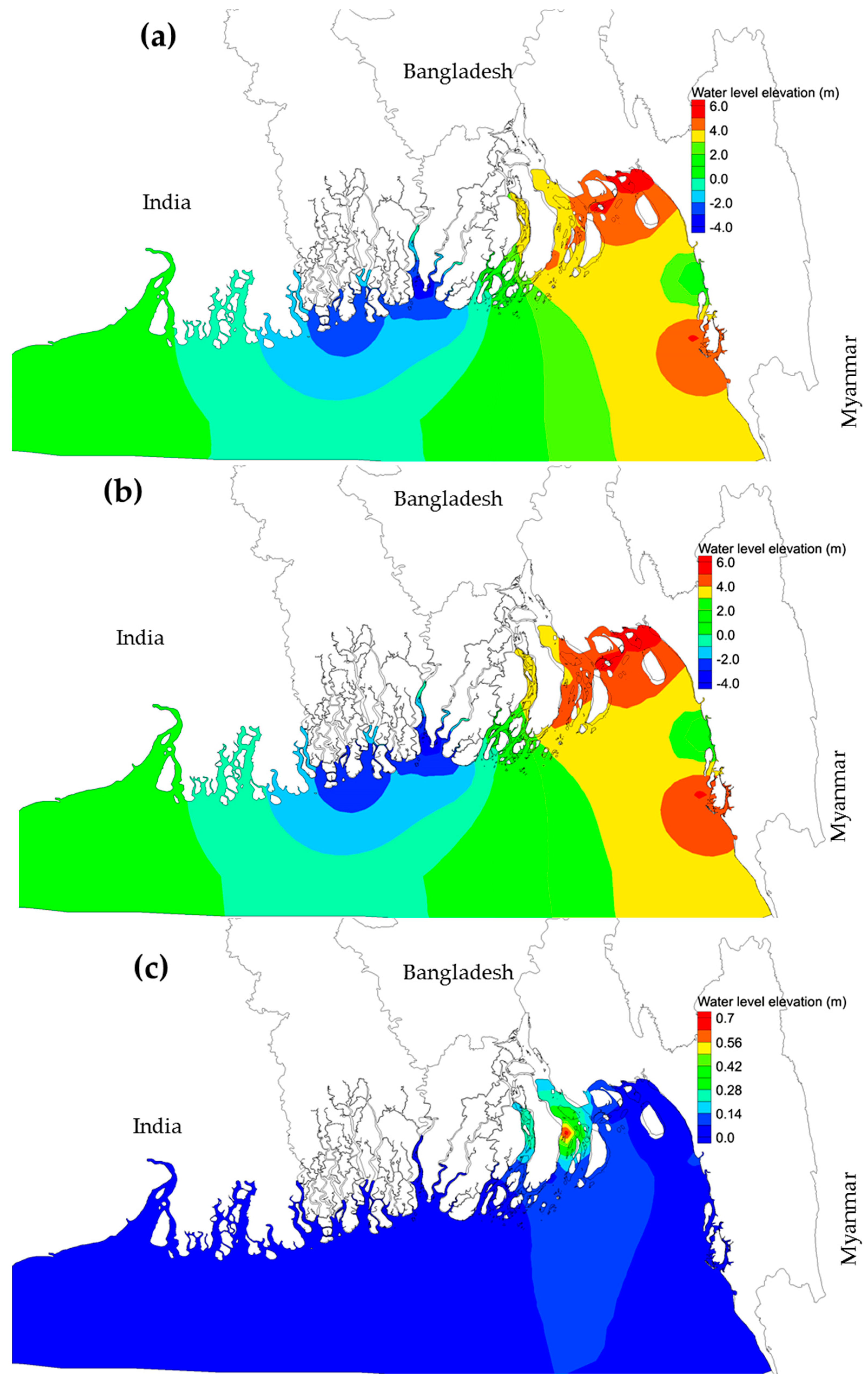
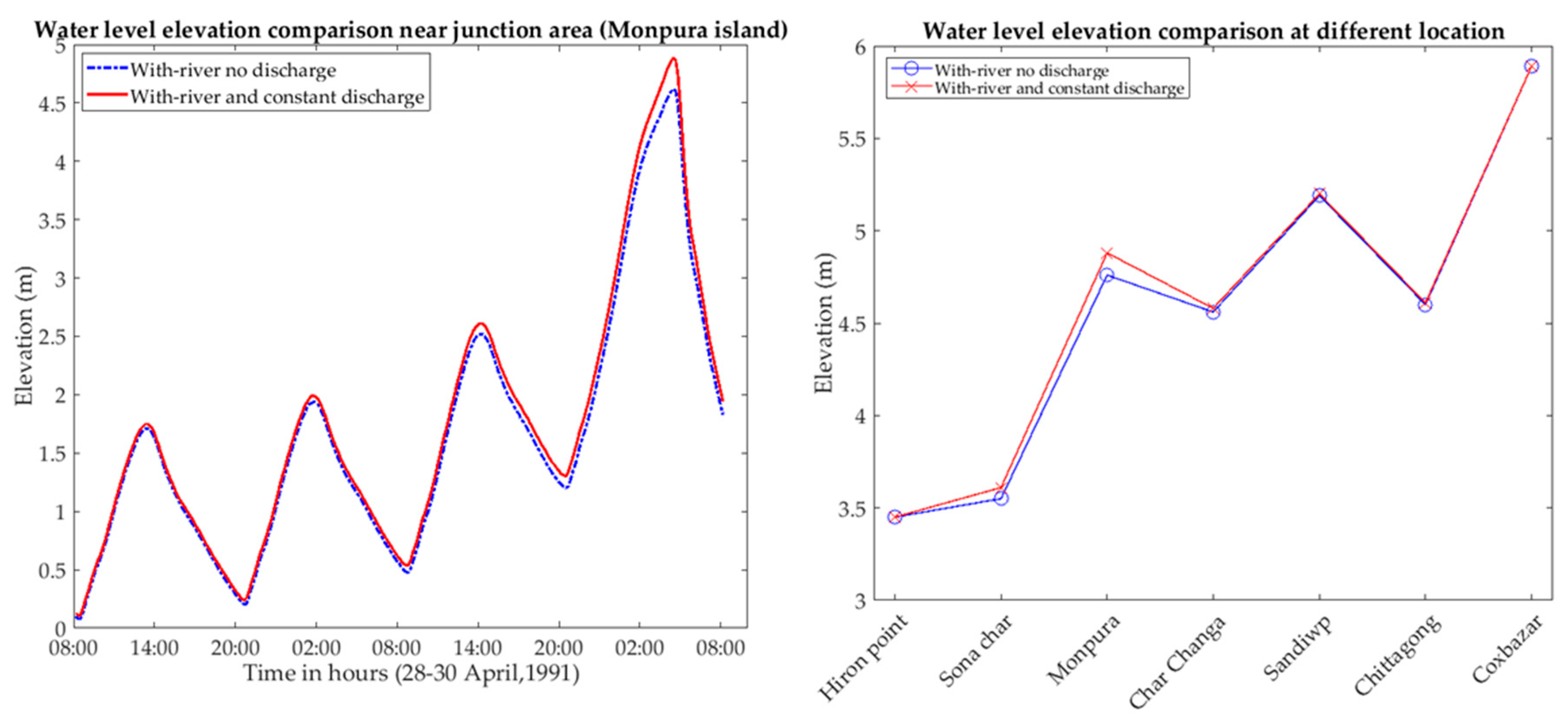
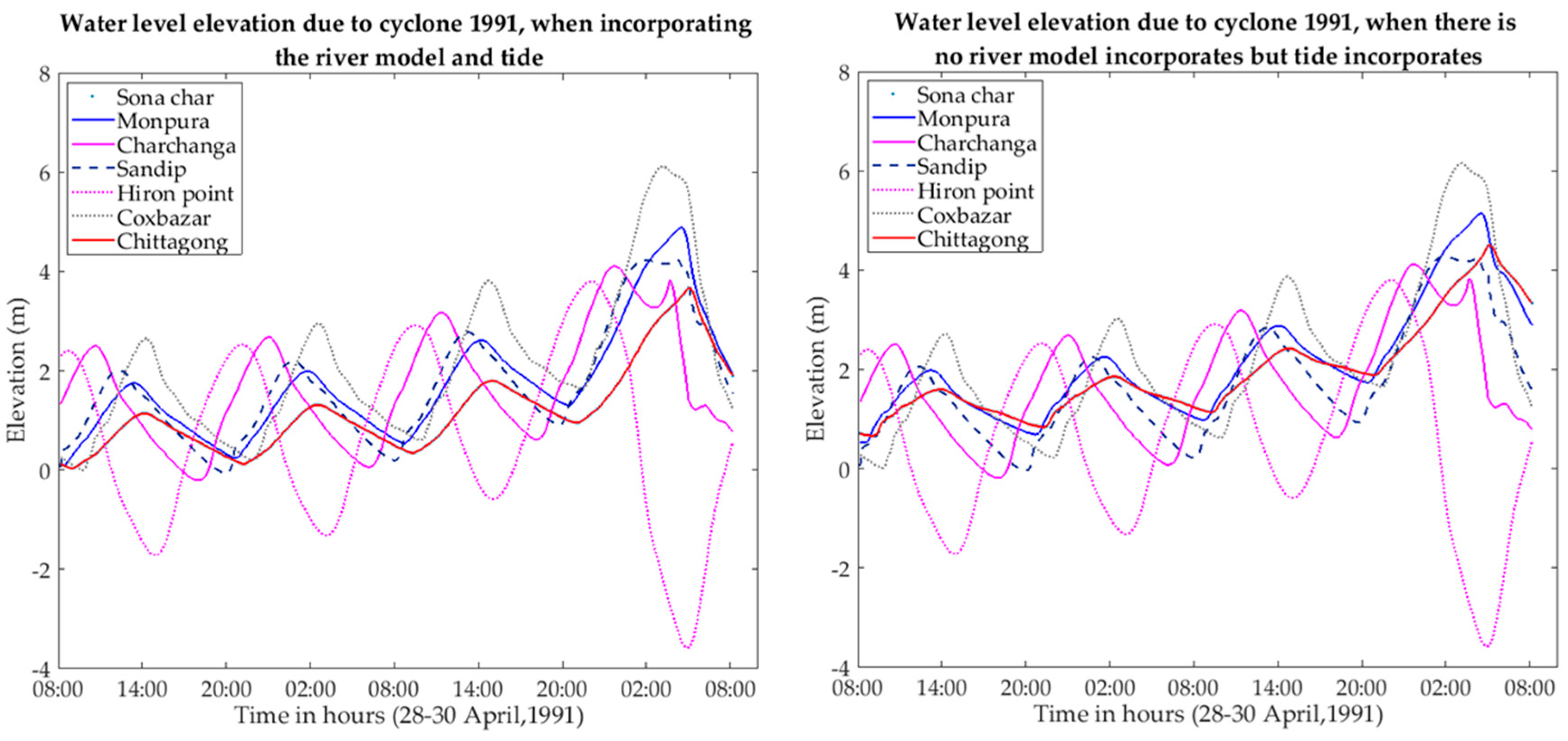
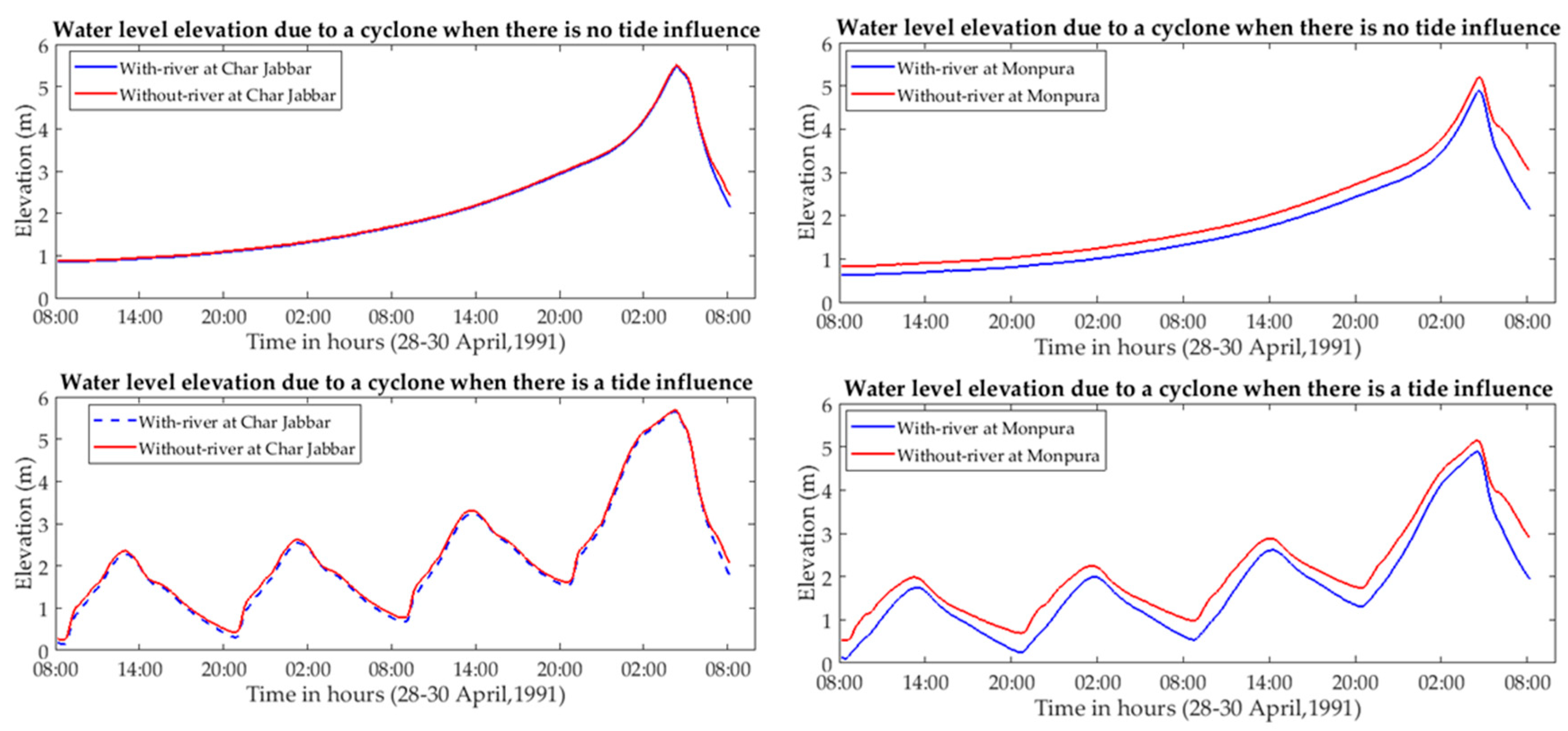
5.1. Model Results
5.2. Results Discussion
6. Conclusions
Author Contributions
Funding
Acknowledgments
Conflicts of Interest
Appendix A

| Sl | Date | Time | Status | Area of the System | Latitude/Longitude | Bulletin | Distance (km) | Signal |
|---|---|---|---|---|---|---|---|---|
| 01. | 26.05.2017 | Afternoon | Low | SE Bay and adjoining Central Bay | - | - | - | - |
| 02. | 27.05.2017 | Afternoon | WML | SE Bay and adjoining Central Bay | - | - | - | - |
| 03. | 28.05.2017 | 9:00 a.m. (03 UTC) | Depression | SE Bay and adjoining Central Bay | 15.2° N/90.6° E | SWB: 01 | Ctg:790; Cxb:710; Mgl:815; Payra:755 | DC-I for all maritime ports |
| 04. | 28.05.2017 | 12 Noon (06 UTC) | Depression | SE Bay and adj Ctl Bay | 15.2° N/90.6° E | SWB: 02 | Ctg:790; Cxb:710; Mgl:815; Payra:755 | DC-I for all maritime ports |
| 05. | 28.05.2017 | 3:00 p.m. (09 UTC) | Deep Depression | SE Bay and adj Central Bay | 15.4° N/90.6° E | SWB: 03 | Ctg:770; Cxb:690; Mgl:790; Payra:735 | DC-I for all maritime ports |
| 06. | 28.05.2017 | 6:00 p.m. (12 UTC) | Deep Depression | SE Bay and adj Central Bay | 15.7° N/90.7° E | SWB: 04 | Ctg:735; Cxb:655; Mgl:760; Payra:700 | DC-I for all maritime ports |
| 07. | 28.05.2017 | 9:00 p.m. (15 UTC) | Deep Depression | SE Bay and adj Central Bay | 15.8° N/90.8° E | SWB: 05 | Ctg:720; Cxb:640; Mgl:750; Payra:690 | DC-I for all maritime ports |
| 08. | 29.05.2017 (28.05.2017) | Midnight (18 UTC) | Cyclone ‘Mora’ | EC Bay and Adj area | 16.2° N/91.2° E | SWB: 06 | Ctg:670; Cxb:590; Mgl:715; Payra:650 | DW-II for all maritime ports |
| 09. | 29.05.2017 (28.05.2017) | 3:00 a.m. (21 UTC) | Cyclone ‘Mora’ | EC Bay and Adj area | 16.7° N/91.2° E | SWB: 07 | Ctg:615; Cxb:535; Mgl:665; Payra:595 | DW-II for all maritime ports |
| 10. | 29.05.2017 (28.05.2017) | 6:00 a.m. (21 UTC) | Cyclone ‘Mora’ | EC Bay and Adj area | 17.1° N/91.2° E | SWB: 08 | Ctg:570; Cxb:490; Mgl:620; Payra:555 | LW-IV for all maritime ports |
| 11. | 29.05.2017 (29.05.2017) | 9:00 a.m. (03 UTC) | Cyclone ‘Mora’ | EC Bay and Adj area | 17.5° N/91.3° E | SWB: 09 | Ctg: 525; Cxb: 445; Mgl: 580; Payra:510 | Ctg, Cxb- DS-VII Mgl, Pyra- DS-V |
| 12. | 29.05.2017 (29.05.2017) | 12 Noon (06 UTC) | Cyclone ‘Mora’ | EC Bay and Adj North Bay | 17.9° N/91.3° E | SWB: 10 | Ctg: 480; Cxb: 400; Mgl: 540; Payra:470 | Ctg, Cxb- DS-VII Mgl, Pyra- DS-V |
| 13. | 29.05.2017 (29.05.2017) | 3:00 p.m. (09 UTC) | Cyclone ‘Mora’ | EC Bay and Adj North Bay | 18.4° N/91.3° E | SWB: 11 | Ctg: 425; Cxb: 345; Mgl: 490; Payra:415 | Ctg, Cxb- DS-VII Mgl, Pyra- DS-V |
| 14. | 29.05.2017 (29.05.2017) | 6:00 p.m. (12 UTC) | SCS ‘Mora’ | North Bay and adj EC Bay | 18.8° N/91.3° E | SWB: 12 | Ctg: 385; Cxb: 305; Mgl: 450; Payra:370 | Ctg, Cxb- GDS-X Mgl, Pyra- GDS-VII |
| 15. | 29.05.2017 | 9:00 p.m. (15 UTC) | SCS ‘Mora’ | North Bay and adj EC Bay | 19.0° N/91.3° E | SWB: 13 | Ctg: 360; Cxb: 280; Mgl: 430; Payra:350 | Ctg, Cxb- GDS-X Mgl, Pyra- GDS-VII |
| 16. | 30.05.2017 (29.05.2017) | Midnight (18 UTC) | SCS ‘Mora’ | North Bay and adj EC Bay | 19.5° N/91.3° E | SWB: 14 | Ctg: 305; Cxb: 230; Mgl: 380; Payra:300 | Ctg, Cxb- GDS-X Mgl, Pyra- GDS-VII |
| 17. | 30.05.2017 (29.05.2017) | 3:00 a.m. (21 UTC) | SCS ‘Mora’ | North Bay and adj EC Bay | 20.2° N/91.4° E | SWB: 15 | Ctg: 230; Cxb: 150; Mgl: 320; Payra:235 | Ctg, Cxb- GDS-X Mgl, Pyra- GDS-VII |
| 18. | 30.05.2017 (30.05.2017) | 6:00 a.m. (00 UTC) | SCS ‘Mora’ | North Bay | Started Crossing Cox’s Bazar-Chittagong Coast near Kutubdia | SWB: 16 | - | Ctg, Cxb- GDS-X Mgl, Pyra- GDS-VII |
| 19. | 30.05.2017 (30.05.2017) | 12 Noon (06 UTC) | Land Deep Depression | Rangamati and adjoining area | Crossed Cox’s Bazar-Chittagong Coast during 06:00 a.m. to 12 Noon | SWB: 17 | - | Ctg, Cxb- GDS-X Mgl, Pyra- GDS-VII |
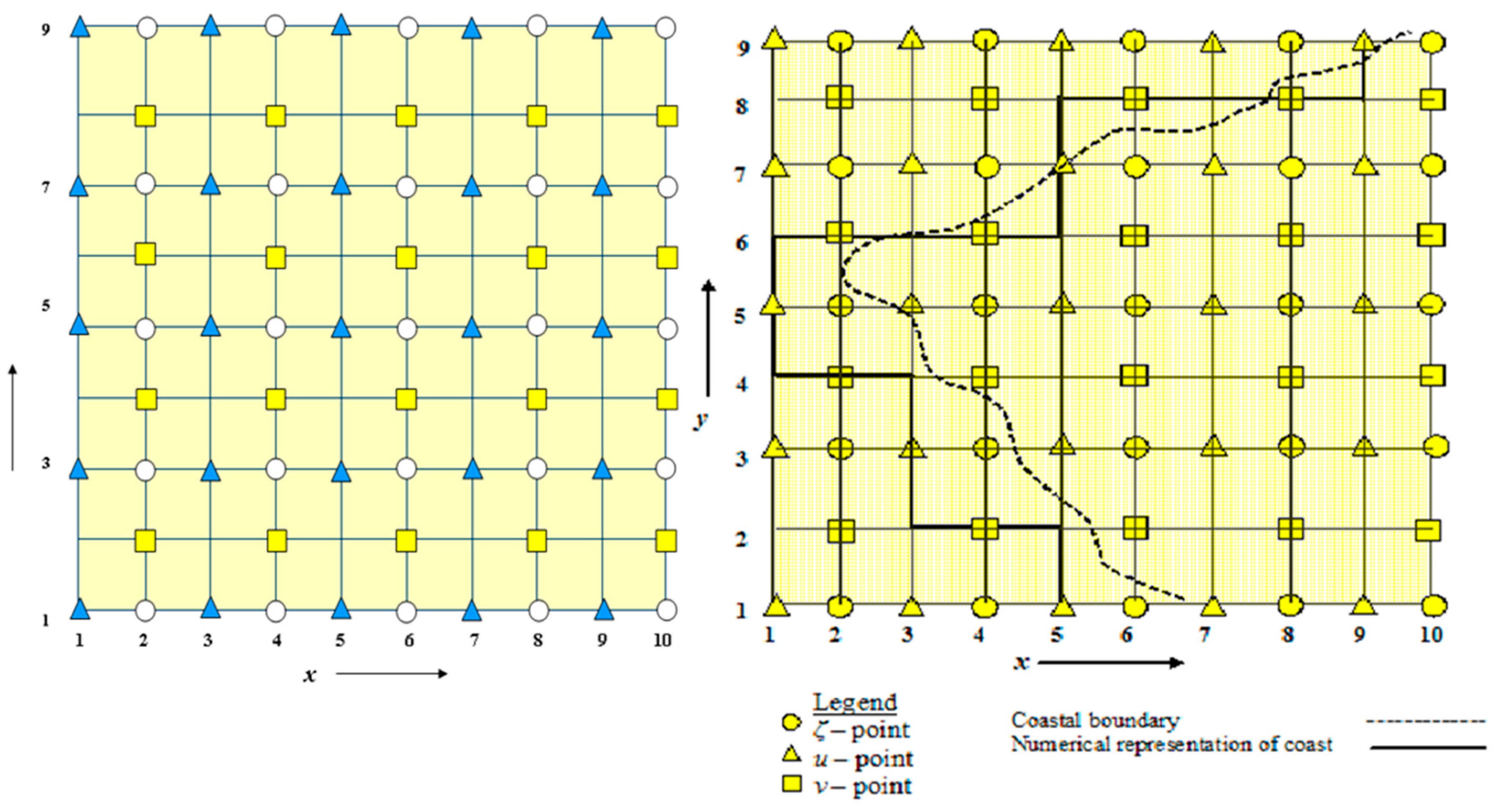
Appendix B. River Model Discretization
References
- Mohit, A.A.; Yamashiro, M.; Ide, Y.; Kodama, M.; Hashimoto, N. Tropical cyclone activity analysis using MRI-AGCM and d4PDF data. In Proceedings of the Twenty-Eighth International Ocean and Polar Engineering Conference, Sapporo, Japan, 10–15 June 2018. [Google Scholar]
- Jelesnianski, C.P. A numerical calculation of storm tides induced by a tropical storm impinging on a continental shelf. Mon. Weather Rev. 1965, 93, 343–358. [Google Scholar] [CrossRef]
- Jelesnianski, C.P. Numerical computation of storm surges without bottom stress. Mon. Weather Rev. 1966, 94, 379–394. [Google Scholar] [CrossRef]
- Thacker, W.C. Irregular grid finite difference techniques for storm surge calculations for curving coastline. Elsevier Ocean Ser. Mar. Forecast. 1979, 261–283. [Google Scholar]
- Mehrdad, S. Storm surge and wave impact of low-probability hurricanes on the lower delaware bay—Calibration and application. J. Mar. Sci. Eng. 2018, 6, 54. [Google Scholar]
- Juan, L.G.; Celso, M.F. Storm surge modeling in large estuaries: Sensitivity analyses to parameters and physical processes in the chesapeake bay. J. Mar. Sci. Eng. 2016, 4, 45. [Google Scholar]
- Kurian, N.P.; Nirupama, N.; Baba, M.; Thomas, K.V. Coastal flooding due to synoptic scale, meso-scale and remote forcings. Nat. Hazards 2009, 48, 259–273. [Google Scholar] [CrossRef]
- Keim, B.D.; Muller, R.A. Hurricanes of the Gulf of Mexico; Louisiana State University Press: Baton Rouge, LA, USA, 2009; p. 216. [Google Scholar]
- Jelesnianski, C.P.; Chen, J.; Shaffer, W.A. SLOSH: Sea, Lake and Overland Surges from Hurricanes; Technical Report for NOAA Technical Report; U.S. Department of Commerce, National Oceanic and Atmospheric Administration, National Weather Service (NWS): Silver Spring, MD, USA, 1992.
- Sheng, Y.P. On modeling three-dimensional estuarine and marine hydrodynamics. Elsevier Oceanogr. Ser. 1987, 45, 35–54. [Google Scholar]
- Sheng, Y.P.; Paramygin, V.A. Forecasting storm surge, inundation and 3D circulation along the Florida coast. In Proceedings of the 11th International Conference on Estuarine and Coastal Modeling, Seattle, DC, USA, 4–6 November 2009; pp. 744–761. [Google Scholar]
- Peng, M.; Xie, L.; Pietrafesa, L.J. A numerical study of storm surge and inundation in the Croatan–Albemarle–Pamlico Estuary System. Estuar. Coast. Shelf Sci. 2004, 59, 121–137. [Google Scholar] [CrossRef]
- Oey, L.; Ezer, T.; Wang, D.P.; Fan, S.J.; Yin, X.Q. Loop current warming by Hurricane Wilma. Geophys. Res. Lett. 2006, 33, 8. [Google Scholar] [CrossRef]
- Chen, C.; Liu, H. An unstructured grid, finite-volume, three-dimensional, primitive equation ocean model: Application to coastal ocean and estuaries. J. Atmos. Ocean. Technol. 2003, 20, 159–186. [Google Scholar] [CrossRef]
- Rego, J.L.; Li, C. On the receding of storm surge along Louisiana’s low-lying coast. J. Coast. Res. 2009, 56, 1042–1049. [Google Scholar]
- Luettich, R.A.; Westerink, J.J.; Scheffner, N.W. ADCIRC: An Advanced Three-Dimensional Circulation Model for Shelves, Coasts and Estuaries. Report 1: Theory and Methodology of ADCIRC-2DDI and ADCIRC-3DL; Technical Report for Dredging Research Program DRP-92-6; US Army Engineers Waterways Experiment Station: Vicksburg, MS, USA, 1992. [Google Scholar]
- Alam, M.; Hossain, A.; Shafee, S. Frequency of Bay of Bengal cyclonic storms and depressions crossing different coastal zones. Int. J. Climatol. 2003, 23, 1119–1125. [Google Scholar] [CrossRef] [Green Version]
- Debsarma, S.K. Simulations of storm surges in the Bay of Bengal. Mar. Geod. 2009, 32, 178–198. [Google Scholar] [CrossRef]
- Paul, G.C.; Ismail, A.I.M. Numerical modeling of storm surges with air bubble effects along the coast of Bangladesh. Ocean Eng. 2012, 42, 188–194. [Google Scholar] [CrossRef]
- Johns, B.; Ali, A. The numerical modeling of storm surges in the Bay of Bengal. Quart. J. R. Met. Soc. 1980, 106, 1–18. [Google Scholar] [CrossRef]
- Roy, G.D. Estimation of expected maximum possible water level along the Meghna estuary using a tide and surge interaction model. J. Environ. Int. 1995, 21, 671–677. [Google Scholar] [CrossRef]
- Roy, G.D. Inclusion of off-shore islands in transformed co-ordinates shallow water model along the coast of Bangladesh. J. Environ. Int. 1999, 25, 67–74. [Google Scholar] [CrossRef]
- Rahman, M.M.; Hoque, A.; Paul, G.C.; Alam, M.J. Nested numerical schemes to incorporate bending coastline and islands boundaries of Bangladesh and prediction of water levels due to surge. Asian J. Math. Stat. 2011, 4, 21–32. [Google Scholar] [CrossRef]
- Lewis, M.; Bates, P.; Horsburgh, K.; Neal, J.; Schumann, G. A storm surge inundation model of the northern Bay of Bengal using publicly available data. Quart. J. R. Met. Soc. 2012, 139, 358–369. [Google Scholar] [CrossRef]
- Paul, G.C.; Ismail, A.I.M.; Karim, M.F. Implementation of method of lines to predict water levels due to a storm along the coastal region of Bangladesh. J. Oceanoger. 2014, 70, 137–148. [Google Scholar] [CrossRef]
- Johns, B.; Sinha, P.C.; Dube, S.K.; Mohanty, U.C.; Rao, A.D. Simulation of storm surge using a three dimensional numerical model: an application to the 1977 Andhra cyclone. Quart. J. R. Met. Soc. 1983, 109, 211–224. [Google Scholar] [CrossRef]
- Dube, S.K.; Singh, P.C.; Roy, G.D. The numerical simulation of storm surges in Bangladesh using a bay-river coupled model. J. Coast. Eng. 1986, 10, 85–101. [Google Scholar] [CrossRef]
- Dube, S.K.; Chittibabu, P.; Sinha, P.C.; Rao, A.D. Numerical modeling of storm surge in the head Bay of Bengal using location specific model. Nat. Hazards 2004, 31, 437–453. [Google Scholar] [CrossRef]
- Agnihotri, N.; Chittibabu, P.; Jain, I.; Sinha, P.C.; Rao, A.D.; Dube, S.K. A Bay–River coupled model for storm surge prediction along the Andhra coast of India. Nat. Hazards 2006, 39, 83–101. [Google Scholar] [CrossRef]
- Milliman, J.D. Flux and fate of fluvial sediment and water in coastal seas. In Ocean Margin Processes in Global Change; Mantoura, R.F.C., Martin, J.M., Wollast, R., Eds.; Wiley: Chichester, UK, 1991; pp. 69–89. [Google Scholar]
- Khalil, G.M. The catastrophic cyclone of April 1991: Its impact on the economy of Bangladesh. Nat. Hazards 1993, 8, 263–281. [Google Scholar] [CrossRef]
- Jain, S.K.; Agarwal, P.K.; Singh, V.P. Hydrology and Water Resources of India; Springer: Berlin, Germany, 2007; ISBN 10 1-4020-5179-4 (HB). [Google Scholar]
- Mills, D.A. A numerical hydrodynamic model applied to tidal dynamics in the Dampier Archipelago. In Bulletin (Western Australia. Dept. of Conservation and Environment) no:190 0156-2983; Perth, W.A., Ed.; Western Australia, Department of Conservation and Environment: Perth, Australia, 1985. [Google Scholar]
- Flather, R.A. A storm surge prediction model for the northern Bay of Bengal with application to the cyclone disaster in April 1991. J. Phys. Oceanogr. 1994, 24, 172–190. [Google Scholar] [CrossRef]
- As-Salek, J.A. Coastal trapping and funneling effects on storm surges in the Meghna estuary in relation to cyclones hitting Noakhali–Cox’s Bazar coast of Bangladesh. J. Phys. Oceanogr. 1998, 28, 227–249. [Google Scholar] [CrossRef]
- Dewan, A.; Corner, R.; Saleem, A.; Rahman, M.M.; Haider, M.R.; Rahman, M.M.; Sarker, M.H. Assessing channel changes of the Ganges-Padma River system in Bangladesh using landsat and hydrological data. Geomorphology 2017, 276, 257–279. [Google Scholar] [CrossRef]
- Islam, M.A.; Mitra, D.; Dewan, A.; Akhter, S.H. Coastal multi-hazard vulnerability assessment along the Ganges deltaic coast of Bangladesh–A geospatial approach. Ocean Coast. Manag. 2016, 127, 1–15. [Google Scholar] [CrossRef]
- Mohit, A.A.; Ide, Y.; Yamashiro, M.; Hashimoto, N. A comparative study of two different numerical methods on storm surge. In Asian and Pacific Coasts 2017, Proceedings of the 9th International Conference on APAC 2017, Pasay, Philippines, 19–21 October 2017; World Scientific Publishing Co. Pte Ltd.: Singapore, 2017; pp. 163–174. [Google Scholar]


| Model | Domain | Grid Spacing along x Axis | Grid Spacing along y Axis | Number of Computational Points |
|---|---|---|---|---|
| CGM | 15° N to 23° N and 85° E to 95° E | 15.08 km | 17.52 km | 60 × 61 |
| FGM | 21°15′ N to 23° N and 89° E to 92° E | 2.15 km | 3.29 km | 92 × 95 |
| VFGM | 21.77° N to 23° N and 90.40° E to 92° E | 720.73 m | 1142.39 m | 190 × 145 |
| VFGMR | 23° N to 23.25° N and 90.40° E to 90.68° E | 720.73 m | 1142.39 m | 40 × 27 |
| Coastal Location | Overall Max. Water Level (m) by [25] | Simulated Overall Max. Water Level (m) by [22] | Simulated Overall Max. Water Level (m) by FDM [38] | Simulated Overall Max. Water Level (m) (without River) | Simulated Overall Max. Water Level (m) (with River) | Observed Overall Max. Water Level (m) |
|---|---|---|---|---|---|---|
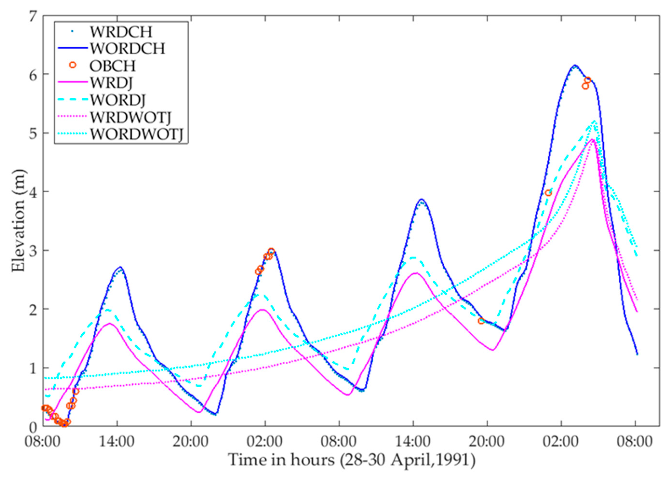
| Cox’s Bazar | -- | -- | 6.14 | 5.98 | 5.89 | 6.00 |
| Moheshkhali | -- | -- | 4.12 | 4.59 | 4.57 | -- |
| Banshkhali | -- | -- | 3.58 | -- | -- | -- |
| Chittagong | 6.25 | 5.45 | 4.50 | 4.60 | 4.61 | 5.4 |
| Sitakunda | 5.78 | -- | 4.48 | 5.15 | 5.11 | -- |
| Sandwip | 5.63 | 5.33 | 4.38 | 5.21 | 5.20 | -- |
| Mirsharai | -- | -- | 5.66 | 5.05 | 5.03 | -- |
| Companiganj | 7.28 | -- | 6.15 | 5.90 | 5.89 | 6.1 |
| Chital Khali | -- | -- | 4.50 | -- | -- | -- |
| Char Jabbar | 6.35 | 5.18 | 5.69 | 5.51 | 5.47 | -- |
| Char Changa | 5.81 | 4.31 | 4.12 | 4.60 | 4.58 | -- |
| Char Madras | 5.81 | -- | 4.32 | 4.99 | 4.95 | -- |
| Rangabali | 4.50 | -- | 4.07 | 3.56 | 3.56 | -- |
| Kuakata | 3.86 | -- | 3.96 | 3.60 | 3.58 | -- |
| Patharghata | -- | -- | 4.36 | 3.55 | 3.57 | -- |
| Tiger Point | 4.57 | -- | 4.21 | 4.30 | 4.30 | -- |
| Hiron Point | 4.01 | 0.70 | 3.80 | 3.48 | 3.45 | 3.5 |
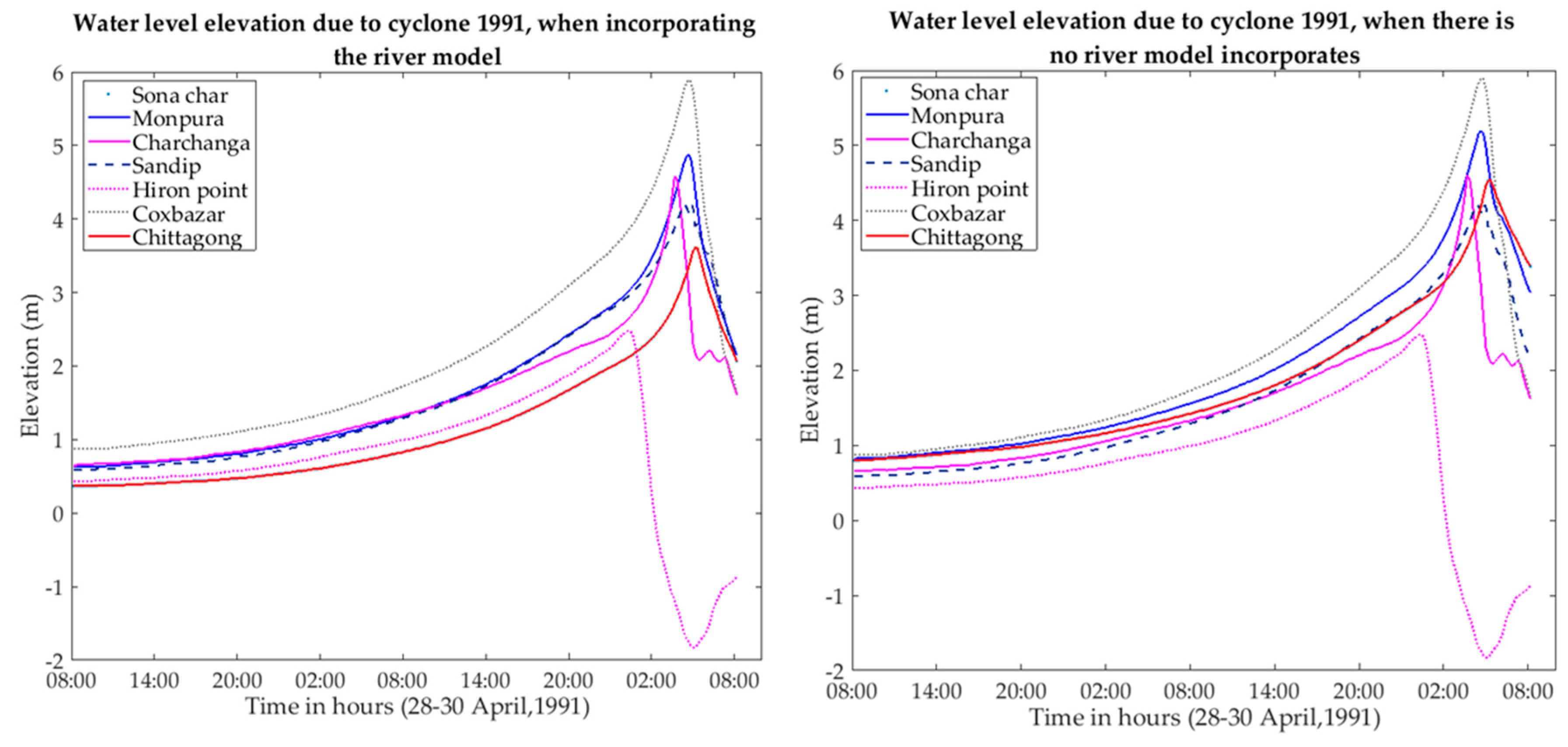
| Monpura Island | -- | -- | -- | 5.20 | 4.88 | -- |
| Sona Char | -- | -- | -- | 4.51 | 3.61 | -- |
© 2018 by the authors. Licensee MDPI, Basel, Switzerland. This article is an open access article distributed under the terms and conditions of the Creative Commons Attribution (CC BY) license (http://creativecommons.org/licenses/by/4.0/).
Share and Cite
Mohit, M.A.A.; Yamashiro, M.; Hashimoto, N.; Mia, M.B.; Ide, Y.; Kodama, M. Impact Assessment of a Major River Basin in Bangladesh on Storm Surge Simulation. J. Mar. Sci. Eng. 2018, 6, 99. https://doi.org/10.3390/jmse6030099
Mohit MAA, Yamashiro M, Hashimoto N, Mia MB, Ide Y, Kodama M. Impact Assessment of a Major River Basin in Bangladesh on Storm Surge Simulation. Journal of Marine Science and Engineering. 2018; 6(3):99. https://doi.org/10.3390/jmse6030099
Chicago/Turabian StyleMohit, Md. Abdul Al, Masaru Yamashiro, Noriaki Hashimoto, Md. Bodruddoza Mia, Yoshihiko Ide, and Mitsuyoshi Kodama. 2018. "Impact Assessment of a Major River Basin in Bangladesh on Storm Surge Simulation" Journal of Marine Science and Engineering 6, no. 3: 99. https://doi.org/10.3390/jmse6030099