1. Introduction
In a world where only 5% of the oceans has been explored, the challenges of underwater exploration is driving the development of new technologies. The barrier of deep-water exploration, not reachable by humans, has been removed by the emergence of underwater robotics. Remotely operated vehicles (ROVs) were one of the first robotics systems used to survey underwater environments. Using artificial intelligence, autonomous underwater vehicles (AUVs) are one of the main systems being developed and constantly improved on to explore and survey deep-waters. The real challenge is to interact with the environment. To solve this a robotic manipulator is added to the underwater vehicle, the complete system being referred to as an underwater vehicle-manipulator system (UVMS).
Underwater vehicle-manipulator systems are highly complex systems, characterized by a large number of degrees-of-freedom, coupled and non-linear dynamics [
1]. The dynamics of the system are highly affected by the dry mass ratio between the two subsystems that form the UVMS. In the case when the vehicle has a considerable mass with respect to the manipulator, e.g., SAUVIM UVMS [
2], the effects of the manipulator motion are not significant. This is not true if the manipulator is attached to a light vehicle. This type of structure is known as a lightweight underwater vehicle-manipulator system [
3]. Using this type of system presents challenges regarding the stability of the robot and simple control laws are not sufficient to perform the required tasks. While extensive research for vehicle-manipulator systems in aerial domain has been made in recent years [
4,
5,
6], studies of underwater vehicle-manipulator systems are still limited due to the high operational costs and need of large infrastructure facilities.
Interaction tasks in the underwater environment using a lightweight vehicle-manipulator system are highly challenging and research in this area is slowly developing. Most of the available literature is based on classic force control approaches: impedance, hybrid or parallel control. Impedance control is based on the dynamic relationship between the position and the force variable, controlling one of them through the other [
7]. Hybrid control is based on the assumption that ideal conditions are available in the robot space and the task that has to be performed by the robot can be defined in two separate orthogonal and complementary directions covering the 3D space [
8]. The parallel control approach combines a motion controller and a force controller. It is claimed to increase the robustness of the force/position control as it incorporates the advantages of both the impedance and hybrid control. It is as simple and robust as the impedance control and enables the control of the position and force separately [
9]. The difficulties encountered in the interaction between the UVMS and the environment include uncertainties in the UVMS model knowledge, the hydrodynamic effects, redundancy of the system, the coupling effects between the manipulator and the vehicle and the effects on the vehicle stability when interacting with the environment. Most of these challenges have been analyzed in the available literature. In [
10] the authors present the impedance controller for an UVMS considering it as a single dynamic system. An adaptive impedance controller is used together with a hybrid controller in [
11]. The system switches between the two controllers by using a fuzzy logic approach. The authors argue that using both types of controllers is beneficial for systems where uncertainties are present in the system.
Underwater vehicle-manipulator systems can be controlled at a low-level either in the operational space or in the vehicle/joints space. Two main categories of control strategies for complex systems can be identified. One approach investigates a separate type of controller for the vehicle and another type of controller for the manipulator. McLain et al. [
12] presents a coordinated-control approach for a UVMS having a single link manipulator. A separate feedback controller for the vehicle and a different controller for the manipulator are designed and the hydrodynamic model of the manipulator is used to coordinate and reduce the effects of the manipulator on the vehicle. Vehicle control can be achieved with advance strategies such as a sliding-mode control system using a direction-based genetic algorithm and fuzzy inference mechanism [
13,
14]. Among the control structures specific to underwater environments Simetti et al. proposes the use of task priority control [
15]. Wit et al. [
16] approaches the issue of different bandwidth properties for the vehicle and manipulator. A Proportional-Derivative controller is implemented for the manipulator whose gains are limited according to the bandwidth of the manipulator. A similar problem is solved in the paper of Kim et al. [
17] where the UVMS is presented as a decentralized system. A proportional vehicle controller is designed in operational space and a feedback linearised controller is used for the manipulator. A different group of control strategies for a UVMS includes a single type of controller designed for the overall system. In most cases, the control law is designed in the operational space. Antonelli et al. [
18] proposes the use of a sliding-mode controller (SMC) to track a desired trajectory with the UVMS. The method is advantageous for the system as there is no need to have an exact dynamic model as the method handles uncertainties and disturbances. In [
19] the authors present a comparison between an operational-space sliding mode controller and a classical Proportional-Derivative Operational Space Controller. The advantages of the SMC can be observed through the simulation results.
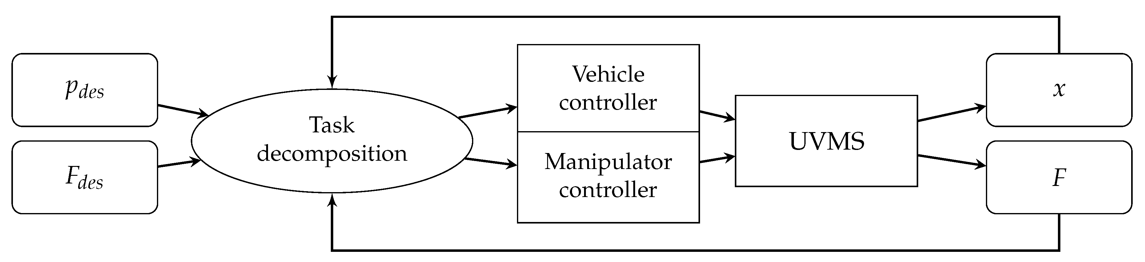
The contribution of this paper is the first extensive comparative analysis between the two main types (coupled and decoupled) of implementing force/position control laws for a lightweight vehicle-manipulator system. The evaluation aims to study the differences between the case when the proposed controller is applied in a centralized (coupled) strategy with the case when a descentalized (decoupled) strategy is used. The coupled strategy allows coordinated movement of the vehicle and manipulator while the decoupled strategy represents a method where movement of the manipulator is restricted during the motion of the vehicle. Moving the vehicle and manipulator simulataneously in the deacoupled strategy would be valid only if at any moment in time the object to be reached is in the workspace of the manipulator. In most real case scenarious of mobile manipulation, the object to be reached is outside of the workspace of the manipulator. This results in the impossibility of controlling just the manipulator, in a deacoupled strategy, before the vehicle brings the manipulator in an area where the object is its manipulation space. Furthermore, if simultaneous movement is desired, this would lead to a coupled control structure as presented in
Section 3.2.
Details of both strategies are discussed in this paper. The performances of underwater manipulation and the area of manipulability are improved by joining together an underwater vehicle with a manipulator. The additional degrees-of-freedom of the vehicle represent an extension to the system that can be used to compensate for the oscillations and disturbances caused by the underwater environment while maintaining good end-effector pose keeping. This paper aims to use these benefits of the UVMS system for the coupled strategy, while for the decoupled strategy the systems are considered separate and the coupling effects are considered as disturbances. The low-level controller used in both strategies combines the theory of sliding mode control for force regulation and the integrative sliding mode control for position regulation in a parallel implementation. The method is robust to disturbances by incorporating the dynamic model of the underwater vehicle-manipulator system in the control architecture. Reliable and efficient UVMSs are not currently available for performing underwater tasks such as probe sampling and maintenance of underwater oil and gas platforms. Research in this field is scarce mostly due to high costs of developing and deploying these type of systems. Before experimental testing takes place with an UVMS, the concepts have to be tested and analysed based on a simulation environment. It is important to demonstrate the validity of the proposed methods in simulation as this step is essential in reducing the probability of failures and damaging the system. Furthermore, the authors argue that it is important to understand the benefits and limitations of the coupled and decoupled control strategies to be able to choose the appropriate approach based on the application the system has to perform.
The mathematical model of the UVMS is described in
Section 2, followed by the presentations of the coupled and the decoupled control strategies in
Section 3. A comparative evaluation of the two methods is presented in
Section 4 and a discussion based on the comparative simulation results is made in
Section 5. All the mathematical symbols used in this paper are listed in
Appendix A.
2. System Model
In this section the underwater vehicle-manipulator system is presented, including the characteristics of the system, the kinematic relationship between different coordinate frames and the dynamic model used to describe the UVMS.
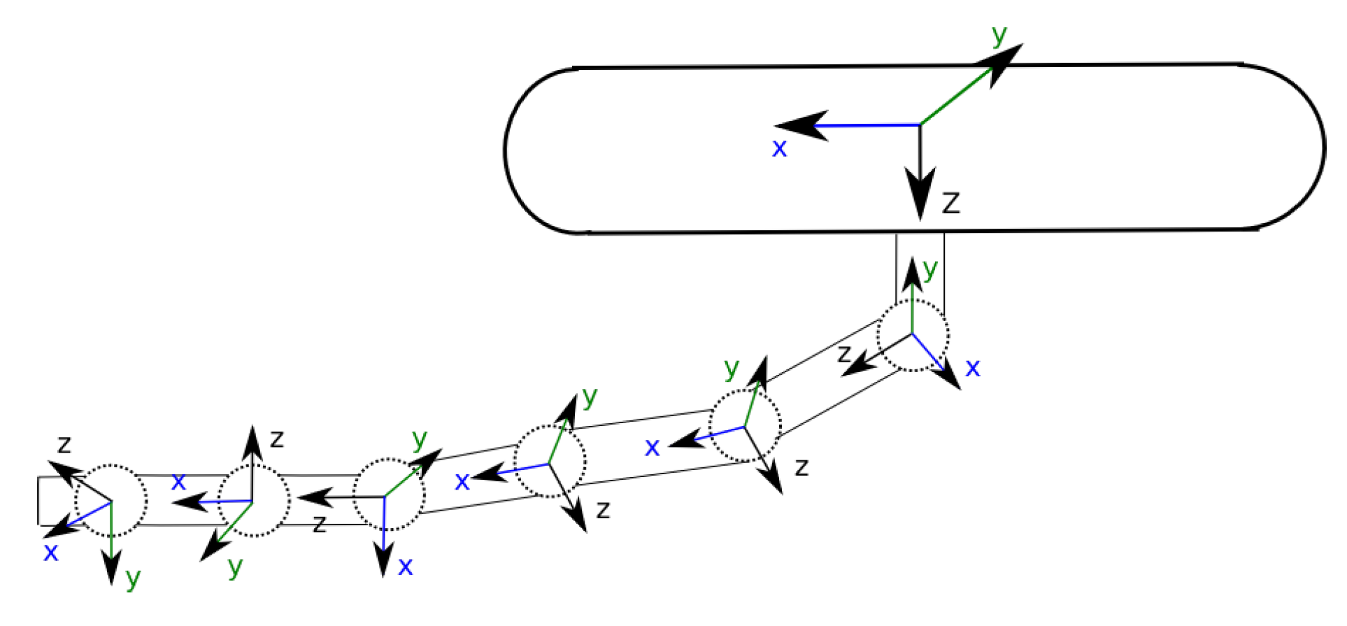
Multiple coordinate systems are available to represent the UVMS: vehicle (body) coordinates, joint coordinates, end-effector (operational/task space) coordinates and earth-fixed inertial coordinates. The kineamtic chain of the proposed UVMS is presented in
Figure 1.
The system position is defined based on the manipulator joint position vector
, vehicle position
and vehicle orientation
. Using the generalized coordinates of the system,
, the end-effector position and orientation
with respect to the inertial frame is given by:
where
is the general transformation dependent on the pose of the vehicle and joint positions. A single chain-representation is used to describe the dynamic model of the underwater-vehicle manipulator based on the work presented in [
20]. This representation is characterised by considering the vehicle to be a part of the manipulator, an extra link with 6 DOFs: 3 prismatic joints and 3 revolute joints. A recursive implementation of the dynamic system as presented in [
21] is used to compute the dynamic model of the system. The classical principle of Newton-Euler that transmits the velocities and forces between subsystem is used to calculate the bias forces. The Composite Rigid Body Algorithm is implemented for determining the inertia matrix of the system. A rigorous analysis of the hydrodynamic effects is performed and the approximated mathematical forces are included into the computation of the dynamic model. A study of the dynamic and hydrodynamic parameters has been made to accurately represent the underwater vehicle-manipulator system. This detailed description of the UVMS model and the corresponding parameters were previously presented in [
21].
The dynamics of the UVMS can be further described in a matrix form by the following equation:
where
is the inertia matrix,
is the Coriolis and Centripetal vector, both consisting of rigid body terms and added mass terms,
is the damping and lift forces vector,
represents the restoring forces,
is the vector of total forces and moments applied to the vehicle
and the torques applied to the manipulator
,
is the Jacobian of the system,
n is the total number of degrees-of-freedom of the system,
l is the number of DOFs of the vehicle and
m is the number of DOFs of the manipulator.
is the external disturbance vector produced by the interaction with the environment, modelled by Equation (
3).
where
is the point of a plane at rest,
is the end-effector position and
is the stiffness matrix of the environment [
22].
In mobile manipulation the tasks to be solved are naturally expressed in task space coordinates. The dynamic description of the system in operational space can be described by Equation (
4) [
8], where
represents the independent parameters vector described in the operational space.
where
is a positive operational space inertia matrix,
is the vector of Coriolis and Centripetal forces,
is the damping vector,
is the vector of restoring forces, all defined in operational space coordinates and
is the vector of generalized forces at the end-effector.
4. Simulation Results
The evaluation of the two strategies is presented through the simulation results highlighting the benefits and drawbacks of both methods. The core analysis is on the two different strategies (coupled vs. decoupled).
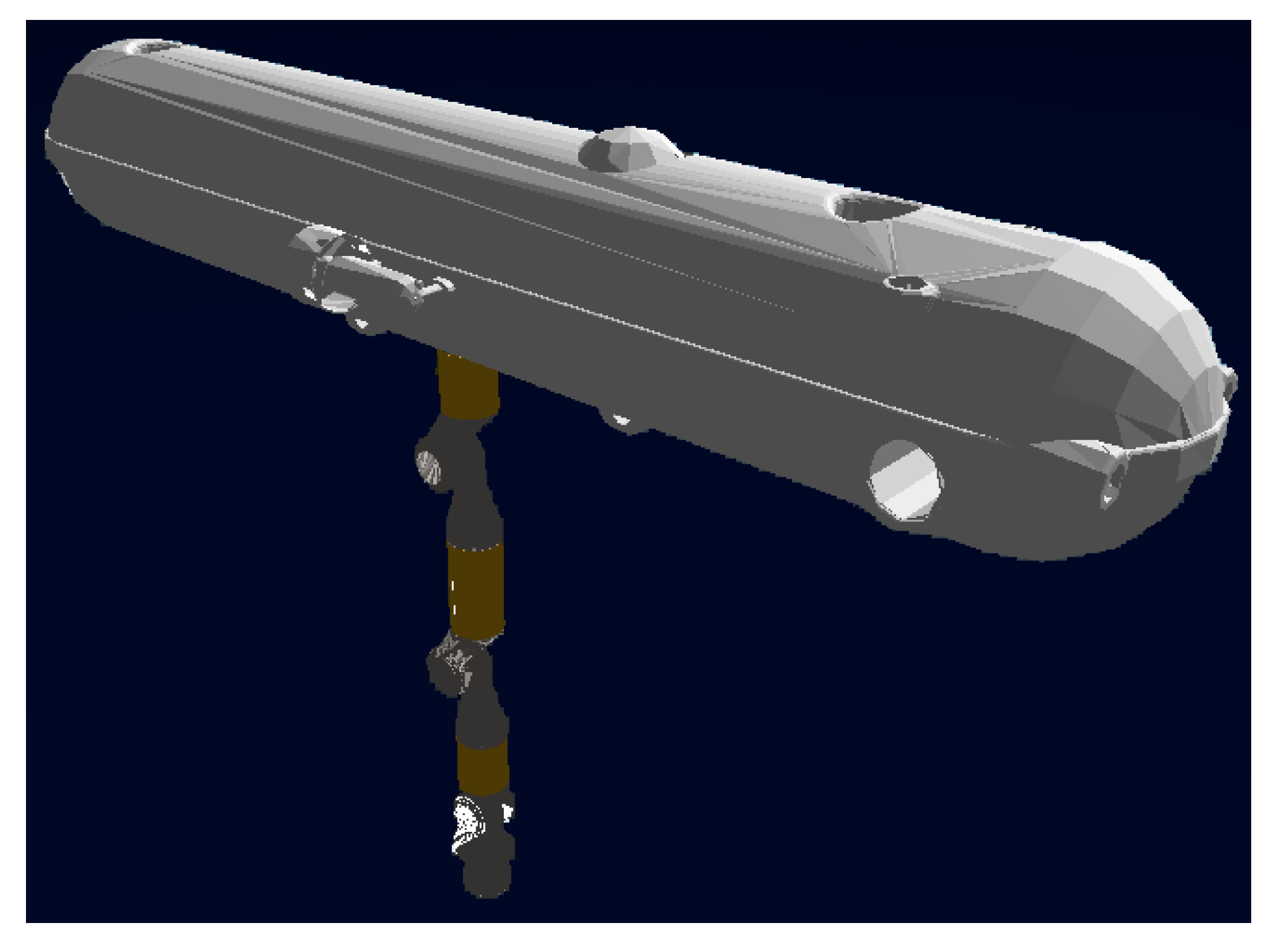
The simulation environment,
Figure 3, is based on an accurate model of the two robotics systems available in the Ocean Systems Laboratory: Nessie VII an autonomous underwater vehicle developed as a research platform and a commercially available underwater manipulator, HDT-MK3-M. Nessie VII AUV is a torpedo shaped 5 degrees-of-freedom vehicle with a mass of 60 kg, a length of
m and a diameter of
m. The vehicle nominal velocity in the translational degrees of freedom is 1 m/s and the angular velocity of the vehicle is
rad/s. The vehicle
degree-of-freedom is not controlled. The manipulator has 6 revolute joints and a total weight of 9 kg. The length of the extended arm is
m and the radius of each link is
m. The manipulator maximum joint velocity for each degree-of-freedom is
rad/s. The system represents a lightweight UVMS characterized by significant effects on the vehicle caused by the manipulator movement.
The system is implemented in Python 2.7.0 using the mathematical model developed in
Section 2 and the control strategies presented in
Section 3. The working frequency for the two systems is 10 Hz, both the vehicle and the manipulator having approximately the same bandwidth. This corresponds to the real hardware systems: both the HDT-MK-3 and Nessie VII cannot be commanded at a higher frequency. As the proposed system operates at low speeds and a reliable model of the system is available, the proposed working frequency is sufficient to generate appropriate control commands. The control parameters used in the implementation of the controller are given in the
Appendix B of the paper.
The problem to be solved is described by the following scenario: the UVMS has to reach a desired object in the underwater environment and interact with it at a predefined force. A compliant, frictionless point-contact at the x-axis of the end-effector describes the interaction force between the end-effector and the object. When the desired final goal is reached the interaction should take place. In these simulations different objects with a variety of stiffness coefficients are used to validate the behaviour of the system. The translational degrees-of-freedom: x, y and z axes of the end-effector are under control. The world coordinates are represented at the point of contact between the base of the manipulator and the vehicle. The end-effector initial position is at m.
The end-effector trajectory between the initial position and object location is described by a cycloid function as defined in Equation (
21). The function represents an interpolation for the position
starting with an initial value
and a desired final value
.
where
4.1. Flexible Environments
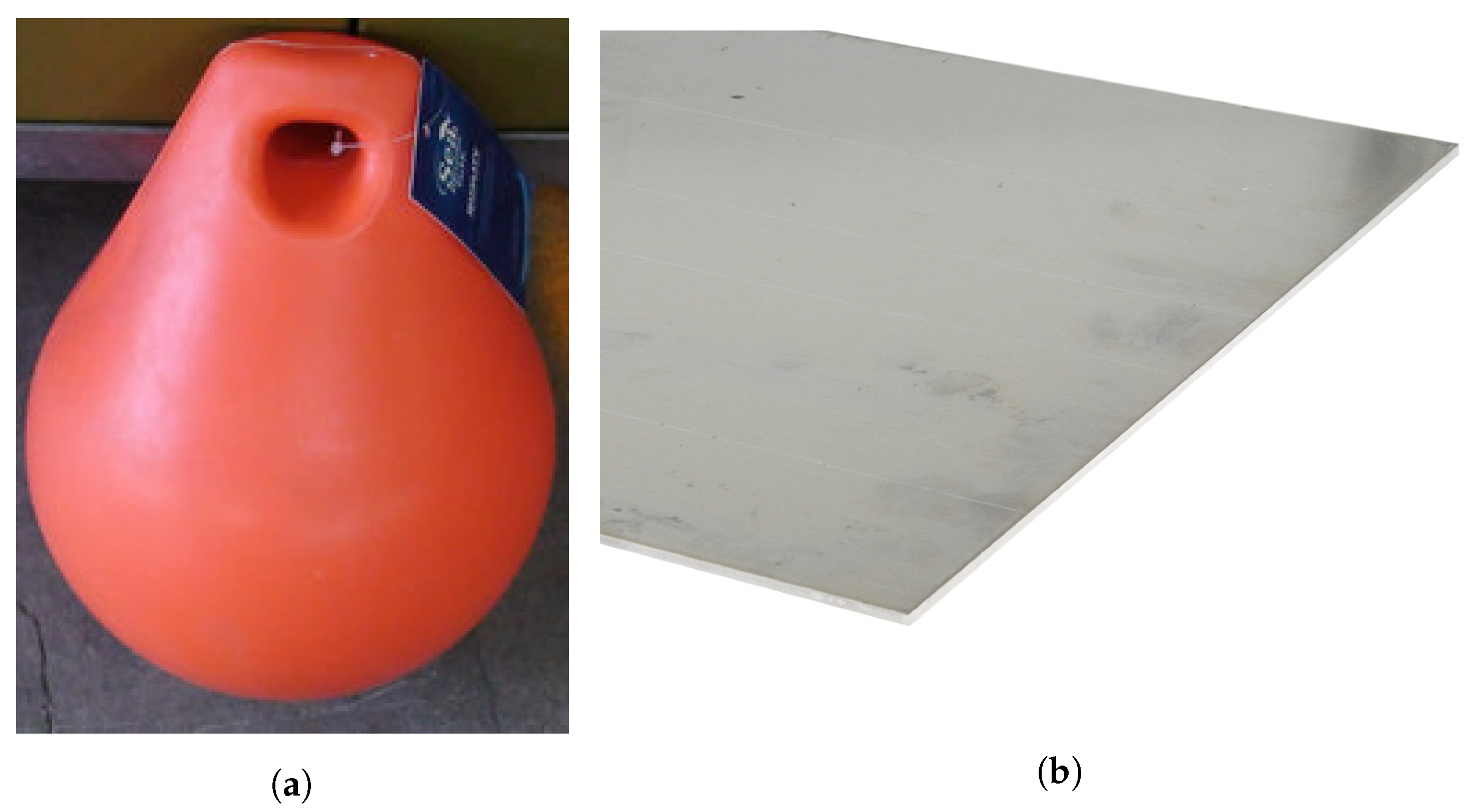
In the first testing scenario it is desired to interact with an object that has a
N/m stiffness coefficient. This stiffness coefficient corresponds to flexible environments, an example of this can be a rubber ball as the one presented in
Figure 4a.
In this case the final goal is
m and the desired interaction force is
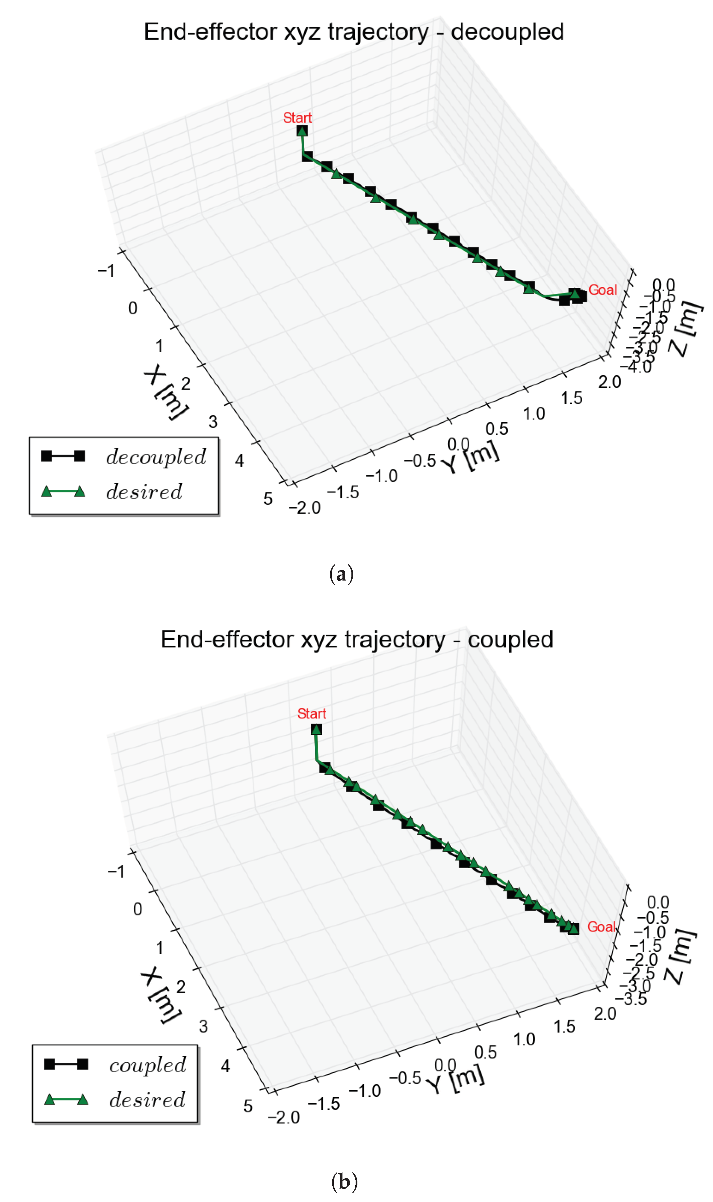
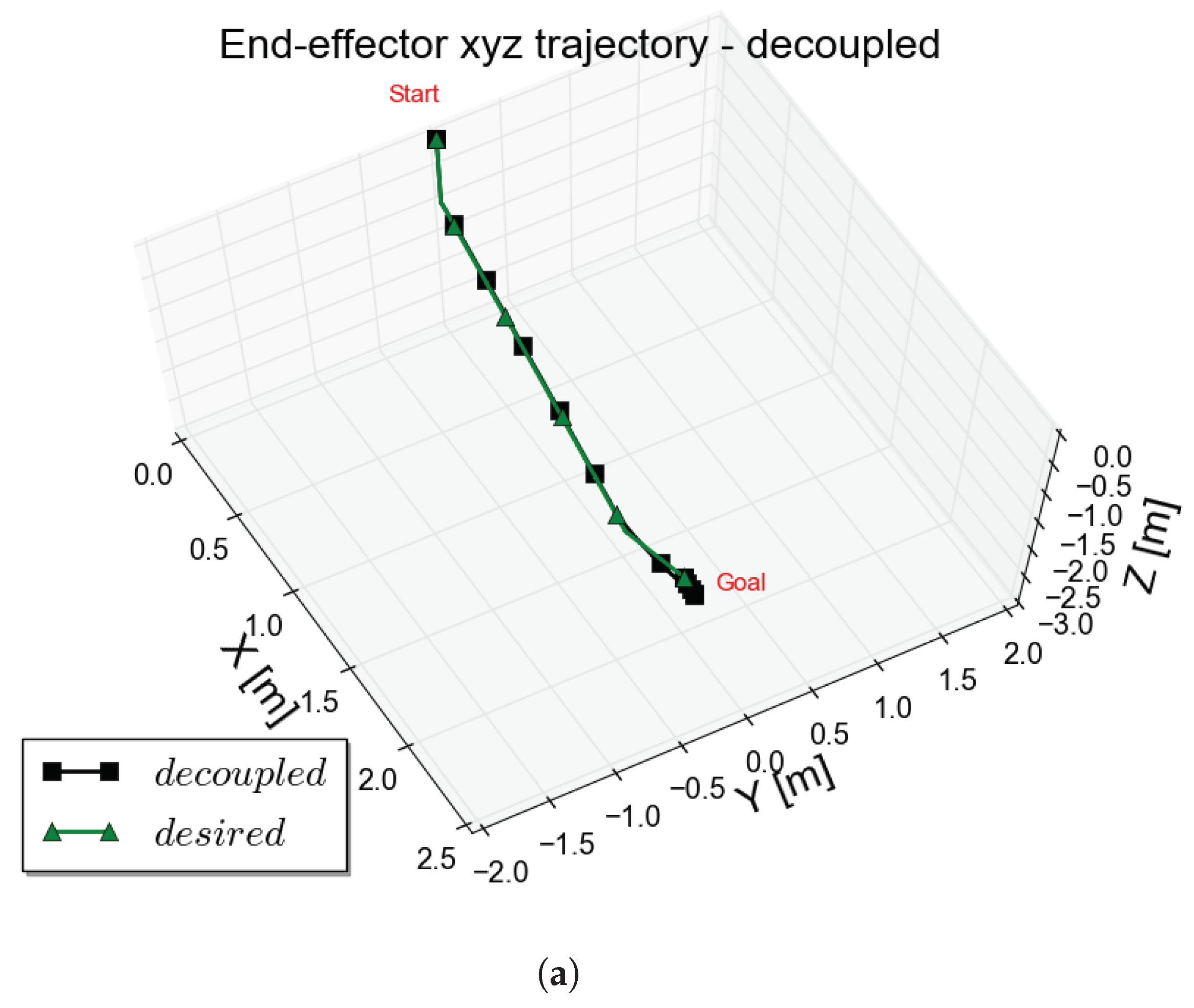
N. The end-effector trajectory tracking is presented in
Figure 5. The desired trajectory starting point is
m in world coordinates that represents the point where the manipulator is attached to the vehicle. Starting at this point, the end-effector is commanded to move towards the goal. The decoupled and coupled strategy behaviour can be observed based on the 3D trajectory of the end-effector.
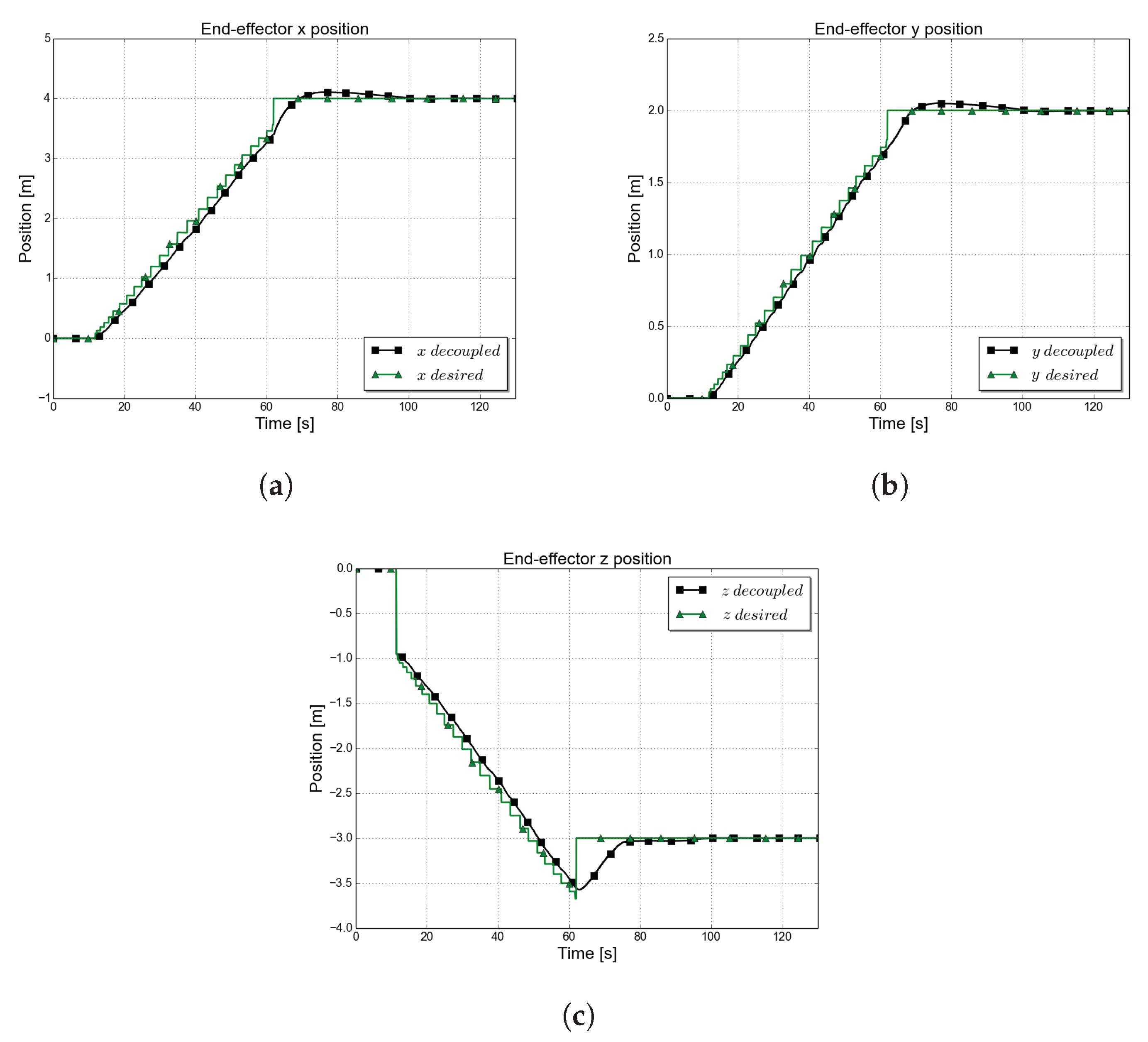
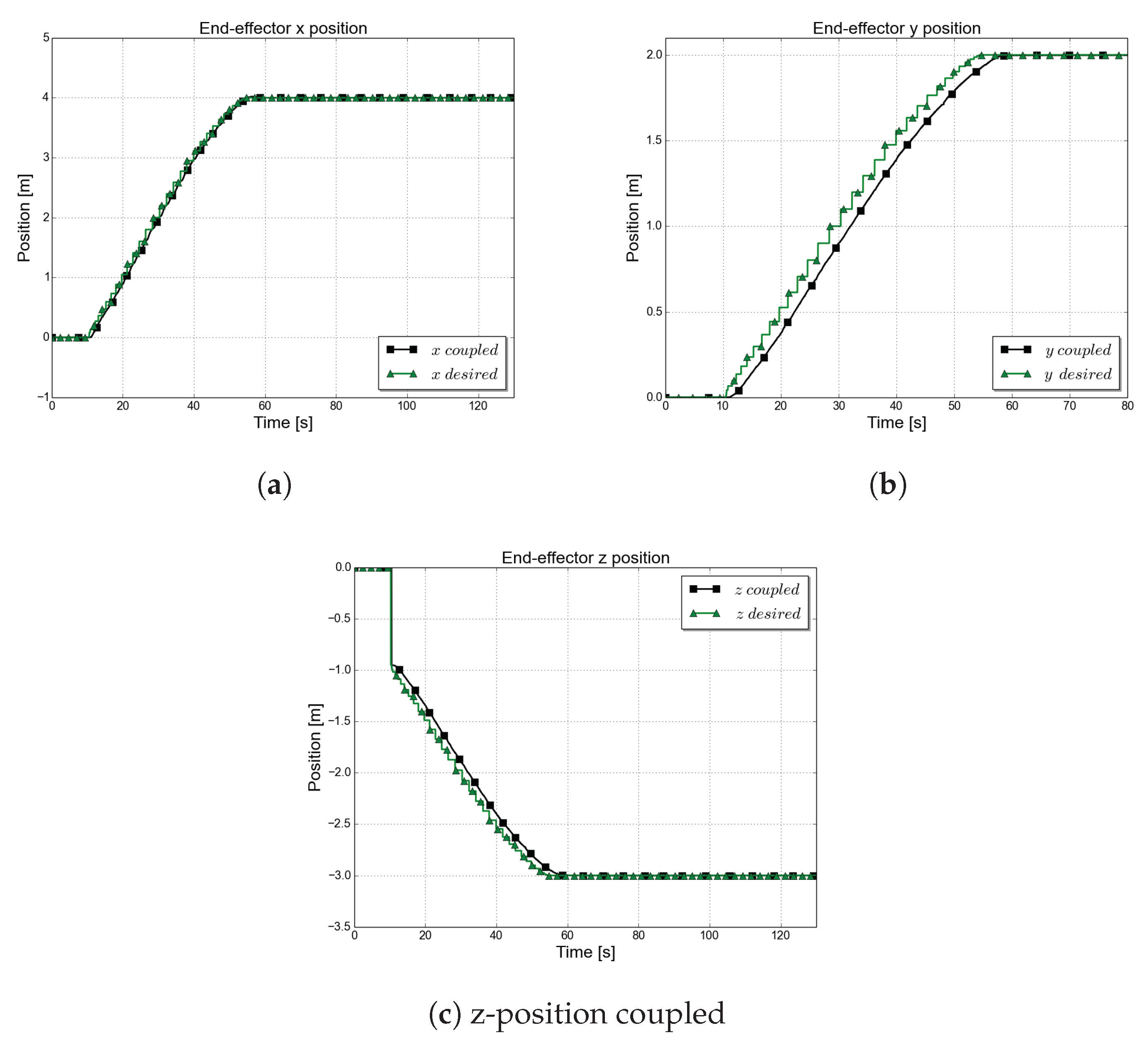
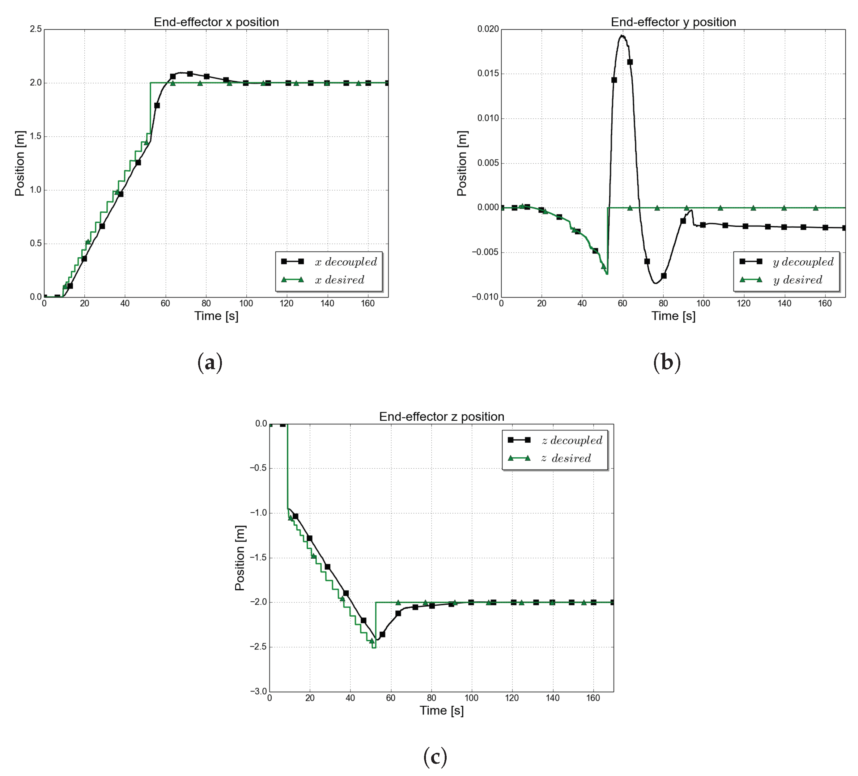
By analysing
Figure 6 and
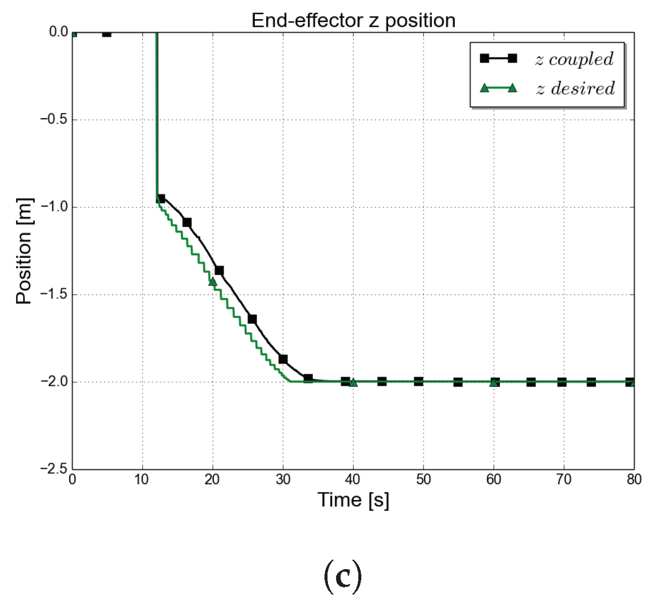
Figure 7a clearer analysis of the behaviour of the end-effector axes can be made. The results are given in the world coordinate system and present the behaviour of the two strategies. Due to the mobile platform the end-effector is able to reach a goal that is placed outside of its fixed workspace. The decoupled approach computes separate goals for the vehicle and manipulator at each time step based on the current location of the vehicle with respect to the goal. This creates a sudden change in the requested end-effector trajectory,
Figure 6c, and is responsible in creating a slower trajectory generation. This represents the main difference in the system behaviour compared with the coupled approach. In the decoupled case, the nature of the system is described by the following behaviour: the vehicle is under control while the manipulator is in station keeping mode until the system reaches the vicinity of the object which the system has to interact with. At the moment when the object is reached the vehicle is in station keeping mode while the manipulator is commanded to move and interact with the object. Using this strategy the end-effector passes beyond the object before it is commanded to move and this causes a different behaviour on the
z-axis in the decoupled strategy compared with the coupled approach. The sudden jump in the
z-trajectory is caused by the selection of the threshold in the decoupled approach. During the vehicle movement, the manipulator is kept in the same configuration as the one seen in
Figure 3. If the vehicle overshoots in
z-axis at the moment when the manipulator starts to move, the trajectory generation module will ask the manipulator to compensate for this overshoot, hence the sudden
z-axis jump in the case of the decoupled approach. Nevertheless, using any of the two strategies, the end-effector trajectory is accurately followed and reliable behaviour is obtained. In the coupled approach, using a single model based controller that handles uncertainties presents good results and the output is comparable with the case when specific controllers are used for each of the systems.
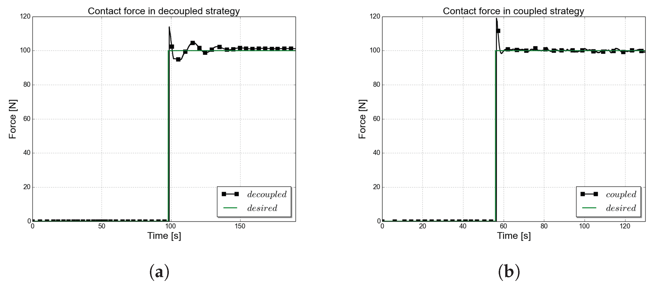
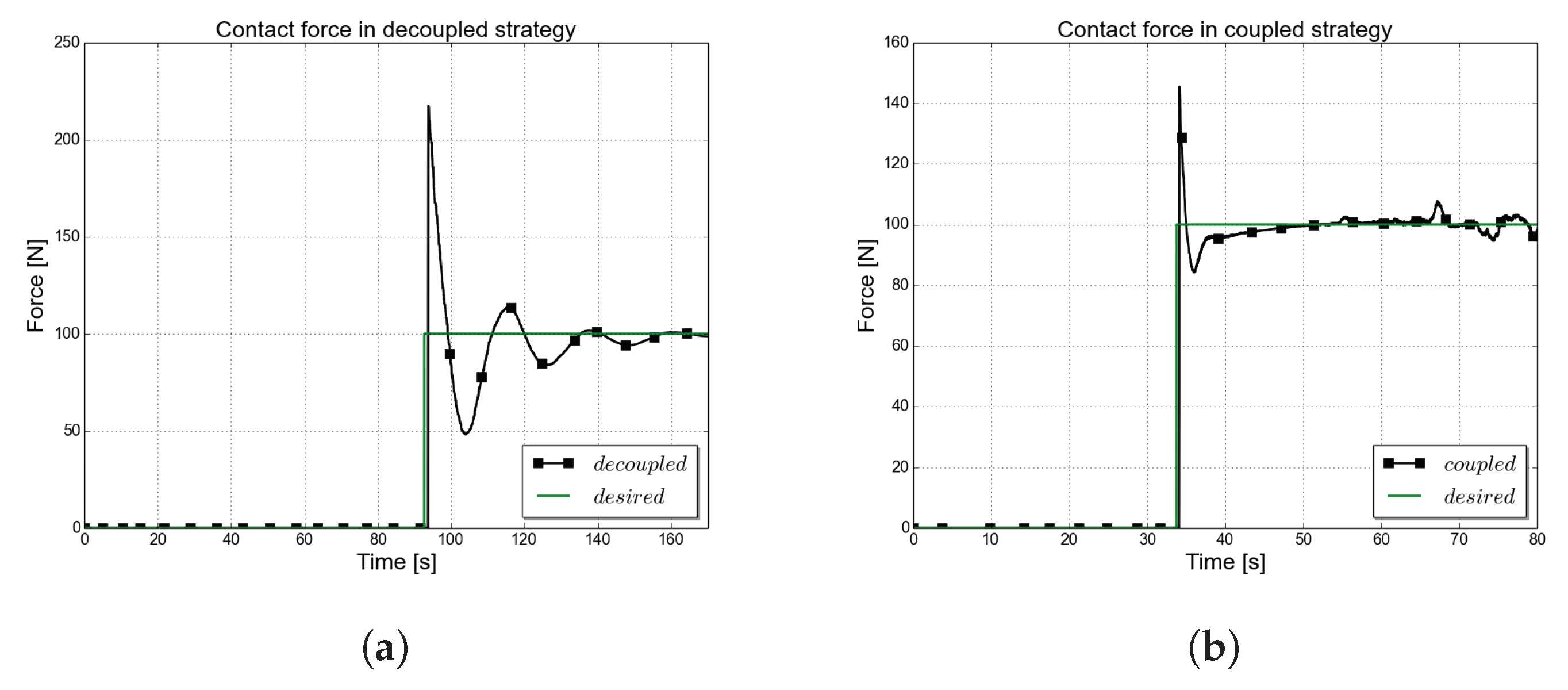
The interaction with the environment,
Figure 8, takes place as soon as the end-effector is within one centimetre of the centre of the object. In the decoupled strategy it can be noticed that the contact with the environment starts at around 90 s, although the system has reached the vicinity of the goal in a similar time as in the coupled case (60 s). This 30 s gap is explained by the overshoot and large time to obtain zero steady-state error. The settling time is large in this approach due to the fact that for a very short time both the vehicle and the manipulator are moving towards the goal. This is caused by a small overshoot in the response when the vehicle controller is used, leading to an overshoot in the overall behaviour of the system.
The desired force is achieved and maintained using both strategies. Small oscillations can be visible in the decoupled approach. For the coupled case an initial larger overshoot is observed but smaller oscillations are seen in
Figure 8b. At the moment when contact with the environment takes place, the manipulator compensates for the force and is trying not to lose position while maintaining contact. This will drive the manipulator to apply a larger force that results in an overshoot.
4.2. Stiff Environments
The second set of experiments presents the interaction between the end-effector and an object with a higher stiffness coefficient,
N/m. This stiffness coefficient corresponds to an aluminum plate sheet as the one presented in
Figure 4b. Based on the results in
Figure 9 it can be observed that the overshoot in the force response increases with the stiffness of the environment. As an integral sliding mode controller is used for the position component, this has priority over the force component and the end-effector position is maintained leading to the overshoot in the force behaviour. Increasing the stiffness of the environment is an additional factor that contributes to the large overshoot.
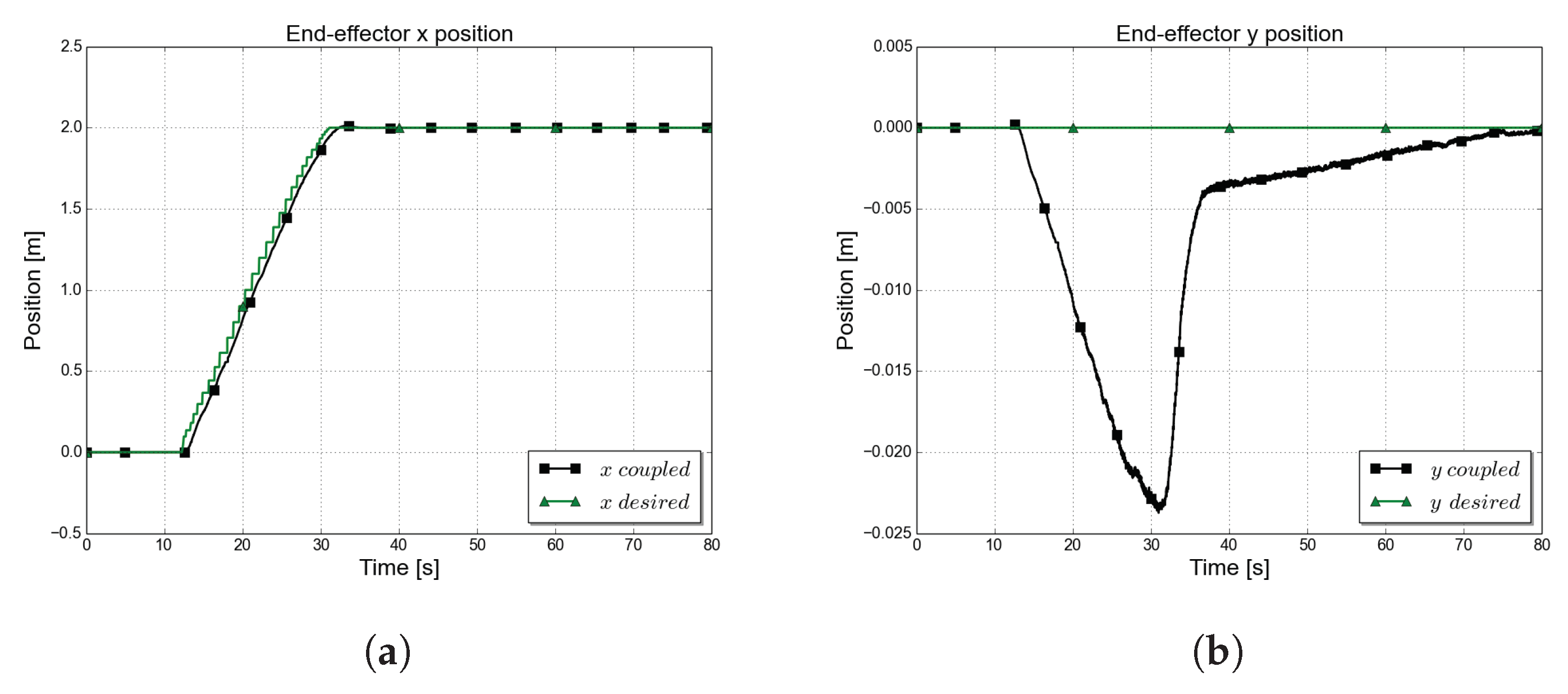
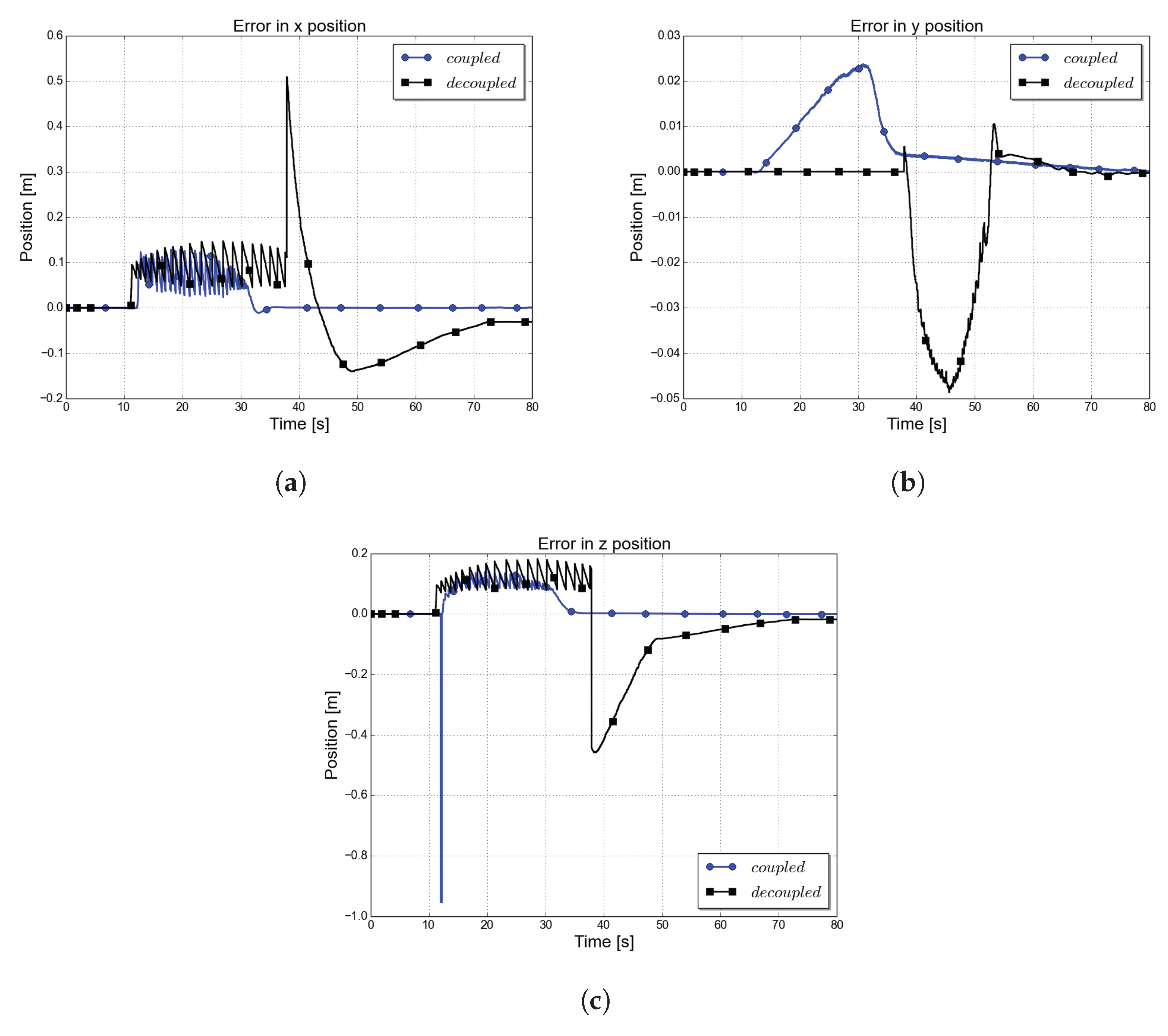
The desired location where contact with an object should take place is set at
m. Looking at the end-effector trajectory tracking,
Figure 10, before the system reaches a steady-state, an overshoot is present in the
x and
y axes. These are caused by using two different controllers for the system. At the moment when the end-effector interacts with a stiff environment large forces affect the system. In the case when the vehicle and manipulator are controlled separately, the vehicle receives these large disturbances and reacts to them by generating a larger control command that will keep the vehicle’s position. Furthermore, the manipulator controller tries to enforce zero steady-state error in position due to the integral term in the control loop and generates large torques. These two elements combined lead to the overshoot in the decoupled strategy behaviour. The coupled approach,
Figure 11, similarly tries to enforce zero-steady state but the large control forces are distributed across the whole system taking into account the full UVMS. Overshoot is present only on a single axis.
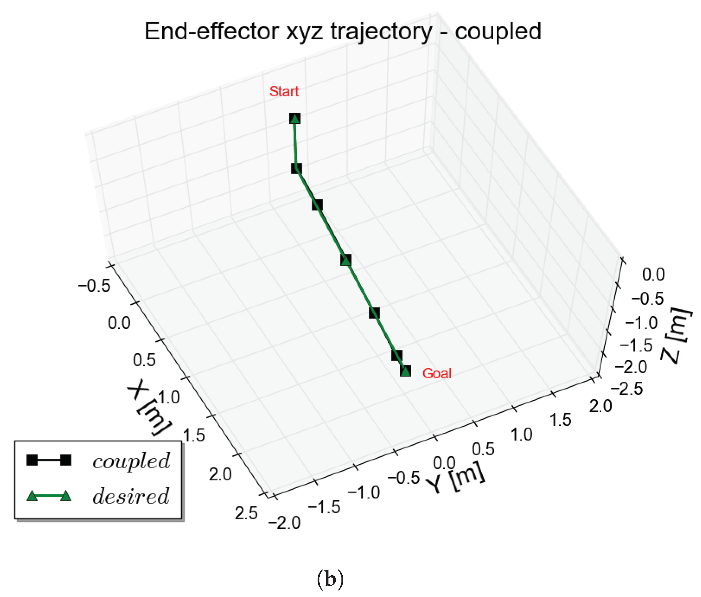
In
Figure 12 the 3D behaviour is presented for the case when the final goal is
m. The goal is reached using any of the two strategies with slightly different behaviour being observed. The coupled strategy is a straightforward approach as the desired trajectory is generated dependent on the end-effector location. In the decoupled strategy the trajectory is generated taking into account the position of the vehicle and the configuration of the manipulator.
5. Discussion
In this paper an operational space parallel position/force controller is used based on the Sliding Mode Control theory and an estimate of the system’s model. The main benefit in using this type of control structure are the reduction of the coupling effects between the light vehicle and the manipulator and a robust response regardless of the uncertainties in the mathematical model or the underwater environment. Using a dynamical sliding-mode control and a continuous function in its implementation leads to a smooth behaviour without chattering effects. The oscillations characteristics to integral sliding mode controllers for the position component of the strategy have been removed with appropriate tuning. Nevertheless, using an integral sliding mode controller gives higher priority to the position component over the force component, resulting in oscillations at the moment of contact when both position and force components are under regulation. These oscillations have a small effect in the first instance of the contact with the environment, but this is rapidly compensated by the control structure producing steady contact and station keeping. The control structure is used in a lightweight vehicle-manipulator system using two different strategies: a centralized method (the coupled approach) and a decentralised structure (the decoupled strategy). Comments are further made regarding the two proposed strategies.
In [
12] the decoupled approach is presented as a classical control strategy for underwater vehicle-manipulator systems where different control laws are used for the vehicle and manipulator. Having a straightforward implementation and being easy to design are the key advantages of this method. By using a robust vehicle control law the disturbances caused by the coupling effects between the vehicle and manipulator are handled as well as the effects of the interaction with the environment. Good trajectory tracking for the end-effector is obtained as well as the desired interaction force with the environment is maintained. One of the key aspects of this strategy is the task decomposition component responsible with distributing what component is active performing movement and which one is kept in station keeping.
When the vehicle is in station keeping it is common that the movement of the manipulator is large, being dependent on the threshold used in the task decomposition component. Setting a very small threshold leads for the vehicle to be in very close proximity to the object while a large threshold may lead for the end-effector to not interact with the environment as the object might be out of reach. Improvements to the decoupled approach can be made using a better tuning for the vehicle controller or by increasing the frequency used for the control loops. Nevertheless, in the results presented, due to the characteristics of the real systems and to obtain a reliable comparison between the two strategies, the same frequency is used for both controllers.
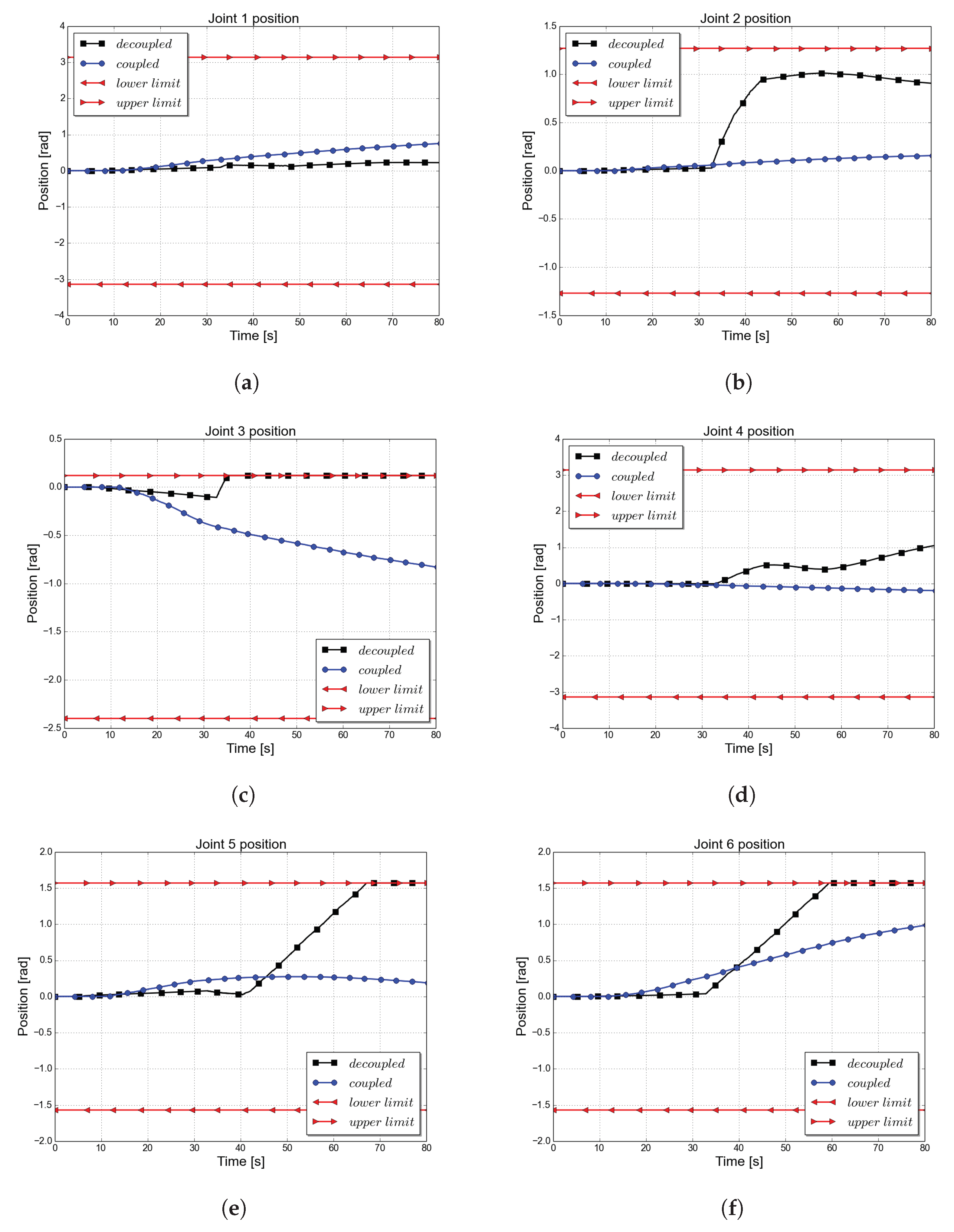
The behaviour of the system using an ill-setted threshold is presented in
Figure 13. As can be seen, the manipulator joints reach their physical limits and a constant error in the steady-state response of the system,
Figure 14, is seen.
Figure 13 presents the behaviour of the joint positions. The physical minimum and maximum limits of the joints are also presented. It was shown in the previous section that this goal,
m, is reachable. In this case it is intended to demonstrate that setting the threshold to half of the manipulator’s length does not lead to the desired behaviour. Furthermore, it is aimed to show that the strategy is sensitive and highly dependent on the threshold used for the task decomposition. Three out of six joints reach their limits,
Figure 13c,e,f and this prevents the end-effector reaching the final goal. The direct connection between the threshold and the success of the task represents a disadvantage of the decoupled approach. Nonetheless, this represents only a naive strategy to decide which subsystem is in station keeping. If a planning strategy such as an optimal trajectory generation approach would be used instead of the cycloid function for waypoints generation improvements in the the system response are expected. Using the dynamic model of the system in the optimal trajectory generation, suitable trajectories can be generated for both vehicle and manipulator, taking into account the interactions between the two subsystems. A detailed description of this type of optimal trajectory generator for UVMS is presented in [
31]. Nevertheless, this is out of the scope of this paper and represents a topic of itself that the authors aim to explore in a future paper.
Figure 13 shows also the behaviour of the joints when the coupled strategy is used. It can be observed that this shows a more restrictive movement of the arm. The joint movements presented in
Figure 13 lead to the end-effector error presented in
Figure 14. It can be seen that the end-effector is locked and a constant
x-axis error is present for the simulation time. In this case, the exact location of the goal is not reached and the manipulator is not in contact with the object with no force being requested to the end-effector.
In the coupled strategy the control law is designed in operational space and the vehicle control forces and the joint torques are generated based on the inverse transformation from task space to joint space. The control system is designed in operational space. The effects of the manipulator movement on the vehicle and the interactions with stiff environments are compensated by incorporating a linearisation technique based on an estimate of the dynamic model. The main advantage of this strategy is the simplicity of the strategy, by using a single controller for the UVMS. In this case there is no need to design an interaction strategy and decide on an appropriate threshold for it. This makes the coupled strategy less sensitive to failure, guaranteeing the success of the task. Another important characteristic is that when using this method the execution time for the task is reduced as the system does not have to evaluate at each time step the distance to the goal and plan accordingly as happens in the decoupled strategy.
Different stiffnesses, from
N/m and
N/m and ten different locations of the goal are used to test the two control strategies. To evaluate the results, the generalized root mean square error in end-effector coordinates, Equation (
22), is used. The evaluation metric is computed separately for the position and force.
N is the number of total measurements and
e is the generalized error. From
Table 1 it can be observed that the performance of the trajectory tracking/position control is independent of the environment stiffness. The overall error in position is improved for the coupled approach, compared with the decoupled strategy. Nevertheless the difference is not significant and the decoupled approach provides accurate trajectory tracking results. For the force error, the coupled approach provides better results than the decoupled strategy. The oscillatory behaviour and the large overshot at high stiffness environments degrades the performance of the decoupled strategy. One specific case is represented by the most compliant environment where the decoupled strategy offers better results than the coupled approach. The object in this case does not oppose high contact forces and the desired force value is reached without any overshoot.
Based on the generalized root mean square error and the relative position error it can be said that the coupled approach performs better in terms of position and force tracking. The error reduction is a result of the use of the overall UVMS dynamic model in the control law and not only for the manipulator. The coupling effects between the manipulator and the vehicle when the system is in contact with the object are handled in this case. The vehicle successfully reacts to these forces facilitating a better position keeping for the end-effector.
One common disadvantage for both strategies rests in the sensitive tuning of the controllers. Not setting the parameters accurately can lead to an oscillatory system or in having a large steady-state error. Tuning the controllers can be challenging as both position and force behaviour have to be accurately obtained. As presented in [
2] tuning operational space controllers is difficult as mapping the control effort from operational space to joint space can produce overshoot in the position-force response or producing a constant-steady state error. Nevertheless, during our simulation it was observed that the most sensitive parameter of both coupled and decoupled methods is the gain,
corresponding to the integral sliding mode controller. Very small variations of this parameter could lead to large oscillatory behaviour and stability loss. Furthermore for having an accurate tracking behaviour the position sliding mode gains
and the force sliding mode gains
were chosen with similar values.
It can be concluded that both strategies can be used on the underwater vehicle-manipulator system. The decoupled strategy represents a controlled method where movement of the manipulator is restricted during the movement of the vehicle. This reduces the risk of collisions with the environment. Using appropriate vehicle and manipulator control structures and reliable interaction strategies, the decoupled method produces similar results to the coupled approach. The main advantage of the coupled approach is the use of a single controller for the overall system as this reduces the coupling effects between the vehicle and manipulator.
It has to be highlighted that the thruster model is not incorporated into this study. According to [
32] this represents a simplification of the system and is a valid approach when the thrusters are used below the critical velocity of the vehicle. This is ensured in our approach as the vehicle that we based our work operates only at low speeds. As mentioned in
Section 4, the simulation system used in this paper is highly representative of a real underwater vehicle and manipulator available in the Ocean System Laboratory, Heriot-Watt University. The control design and operation capabilities have been considered using the physical capabilities of the real vehicle and manipulator system. Implementation of this controller on the real system will only require minor parameter changes, everything else being directly transferable. The underwater currents and the thruster model are the only simplifications made to the real system in the simulation environment. Nevertheless, using an estimate model of the system in the control structure and as sliding mode controllers handle uncertainties and disturbances in the environment ensures that the proposed control structure will be viable on the real system in real underwater environments. Both the vehicle and the manipulator controllers have a sampling a frequency of 10 Hz, the response of the vehicle’s position and orientation transient response being consistent with the transient response from the manipulator.


