Resonantly Forced Baroclinic Waves in the Oceans: Subharmonic Modes


Independent Scholar, 96, rue du Port David, 45370 Dry, France
J. Mar. Sci. Eng. 2018, 6(3), 78; https://doi.org/10.3390/jmse6030078
Submission received: 11 June 2018
/
Revised: 26 June 2018
/
Accepted: 27 June 2018
/
Published: 2 July 2018
Abstract
:The study of resonantly forced baroclinic waves in the tropical oceans at mid-latitudes is of paramount importance to advancing our knowledge in fields that investigate the El Niño–Southern Oscillation (ENSO), the decadal climate variability, or the resonant feature of glacial-interglacial cycles that are a result of orbital forcing. Indeed, these baroclinic waves, the natural period of which coincides with the forcing period, have a considerable impact on ocean circulation and in climate variability. Resonantly Forced Waves (RFWs) are characterized by antinodes at sea surface height anomalies and nodes where modulated geostrophic currents ensure the transfer of warm water from an antinode to another, reflecting a quasi-geostrophic motion. Several RFWs of different periods are coupled when they share the same node, which involves the geostrophic forces at the basin scale. These RFWs are subject to a subharmonic mode locking, which means that their average periods are a multiple of the natural period of the fundamental wave, that is, one year. This property of coupled oscillator systems is deduced from the Hamiltonian (the energy) of the Caldirola–Kanai (CK) oscillator. In this article, it is shown how the CK oscillator, which is usually used to develop a phenomenological single-particle approach, is transposable to RFWs. Subharmonic modes ensure the durability of the resonant dissipative system, with each oscillator transferring as much interaction energy to all the others that it receives periodically.
1. Introduction
The resonance of baroclinic waves in the stratified oceans is a topic that motivates sustained research, be it equatorial or off-equatorial waves. The main areas of interest are (1) the resonant, baroclinic, equatorially-trapped waves [1,2,3,4,5], including the ability of long-wave low-frequency basin modes to be resonantly excited [6]; (2) the resonant excitation of non-dispersive coastal baroclinic waves [7,8]; (3) the resonant interplay of baroclinic waves between the upper and the deep layer [9]; and (4) the resonant Rossby wave motions in the off-equatorial oceans [10,11].
In previous works, the phenomenon of resonance refers to a variety of mechanisms that all share in common the ability to amplify the baroclinic waves. In the context of this study, this concept is restricted to baroclinic waves induced by a quasi-periodic forcing, the resonance phenomenon occurring when the natural period of the baroclinic waves coincides with the period of forcing. Interpreted in this way, the resonance of baroclinic waves in the oceans has been studied very little.
The study of resonantly forced baroclinic waves in the tropical oceans at mid-latitudes is of paramount importance to advancing our knowledge in fields that investigate the El Niño–Southern Oscillation (ENSO), the decadal [12] and, probably, long-term climate variability. Indeed, these baroclinic waves, the natural period of which coincides with the forcing period, have a considerable impact on the climate since the oscillation of the pycnocline depth causes the displacement of warm subsurface water masses. Consequently, ocean-atmosphere interactions are enhanced by increasing the thermal gradient in the upper ocean as well as the moisture content in the atmosphere.
Quasi-periodic forcing has the ability to produce multi-frequency Quasi-Stationary Waves (QSWs). Such waves were highlighted in the Indian Ocean [13,14,15]. They can be observed using the complex empirical orthogonal function [16] or the cross-wavelet analysis [17] of Sea Surface Height (SSH) and Surface Current Velocity (SCV). The amplitude and phase of highlighted anomalies are reproducible from a cycle to another, hence the terminology Quasi-Stationary Waves that recalls the functioning of standing waves.
The resonance requires the adjustment of the natural period of the baroclinic waves to the forcing period. This is for example what occurs in the tropical Pacific during the annual and quadrennial QSWs [18]. It is also what is observed where the western boundary currents leave the continents to re-enter the interior flow of the subtropical gyres, while Rossby waves are embedded in the wind-driven circulation. Geostrophic forces closely constrain the behavior of baroclinic waves at the limits of the basin, forming antinodes at SSH anomalies and nodes where modulated geostrophic currents ensure the transfer of warm water from an antinode to another, reflecting a quasi-geostrophic motion. Although these terms node and antinode are unfair, because the phase of QSWs is not uniform, which supposes some overlapping, the paired figures devoted to the amplitude and phase of these QSWs merely reflect their evolution during a cycle. This terminology recalls that antinodes and nodes are part of the same quasi-periodic dynamical system that corresponds to a particular bandwidth representative of resonant frequencies, whereas the term “anomaly” suggests a transient phenomenon.
The resonant nature of the forced Rossby waves is not fortuitous. Because of the phenomena of friction, only forced waves remain over time, provided the forcing is quasi-periodic. Indeed, a well-tuned configuration on the mean spatial and temporal characteristics of forcing takes full advantage of it, while other less well adapted modes are mitigated. Tuning the resonance frequency according to the periodicity of the forcing will make the amplitude of the oscillation higher and higher (amplitude maximization), while tuning the oscillation at a faster or slower tempo will result in lower amplitude. This is because the energy the oscillation absorbs is maximized when the forcing is ‘in phase’ with the oscillations, while some of the oscillation’s energy is actually extracted by the opposing force of the forcing when it is not. In this way resonant forcing always prevails over non-resonant processes. On the other hand, influence of flow instabilities not related to the periodic forcing is negligible when long-period baroclinic waves are studied.
It is why the resonance of baroclinic waves is ubiquitous [19]. Resulting from the conjunction of first and higher baroclinic mode baroclinic waves, multi-frequency QSWs are superposed. Several meridional mode baroclinic waves can coexist, as this occurs in the tropical Pacific.
Multi-frequency QSWs are endowed with a remarkable property, which gives them a role of primary importance both in ocean circulation and in the variability of climate. Indeed, they have the ability to be coupled when they share the same node, which generally happens both in the tropical and subtropical oceans. The coupling results from the alteration of the geostrophic forces of the basin as a consequence of the convergence and the merging of geostrophic currents.
These different properties make these Resonantly Forced Waves (RFWs) behave like coupled oscillators. In this case a subharmonic mode locking occurs, which means the average periods of coupled QSWs are a multiple of the period of the fundamental wave, that is, the QSW whose natural period coincides with the forcing period. This subharmonic mode locking of QSWs is based on a property of coupled oscillators with inertia. The latter can be modeled in a general way by using equations borrowed from theoretical physics [20].
2. Method
2.1. Wavelet Analysis
This research is focused on the description of multi-frequency resonators applied to ocean dynamics at the planetary scale. The presentation of the results will rely on the wavelet analysis of the SSH and the geostrophic current velocity field in a predetermined frequency band. Incidentally, wavelet analysis has become a common tool for analyzing localized variations of power within a time series. By decomposing a time series into time–frequency space (actually, time-scale space, the period depending on the scale), one is able to determine both the dominant modes of variability and how those modes vary in time.
The wavelet transform has been used for numerous studies in geophysics. Pioneer works include tropical convection [23], the ENSO [24,25], atmospheric cold fronts [26], central England temperature [27], the dispersion of ocean waves [28], wave growth and breaking [29], and coherent structures in turbulent flows [30].
The spatial representation of the Wavelet analysis of the SSH and the Surface Current Velocity (SCV) series allows representing the regions subject to this oscillation phenomenon when the wavelet power is scale-averaged over a relevant band. Here a continuous Morlet wavelet transform is used so that the period and the scale coincide [17,31]. In addition to the wavelet power, it is often necessary to specify the phase that expresses when the oscillation reaches its extrema with respect to a temporal reference. Taking for example the SSH, the cross-wavelet analysis of SSH and the temporal reference (TR) shows the cross-wavelet power and the coherence phase. The cross-wavelet power of SSH and TR divided by the square root of the wavelet power of TR, that is, the normalized cross-wavelet power, coincides with the square root of the wavelet power of SSH. The latter is the amplitude of the SSH oscillation. The coherence phase of SSH and TR shows the time shift between the SSH oscillation and the TR.
Thus, maps are paired; the first is the amplitude of anomalies (regardless of the time when the maximum anomaly occurs), and the second is the phase (the time evolution, that is, the time when the maximum anomaly occurs over a period). The band over which both the cross-wavelet power and the coherence phase are scale-averaged allows taking into account the natural broadening of the frequency bands associated with the oscillations. On both maps, the values at every pixel are processed independently of each other. Therefore, classes are chosen judiciously in relation to the observed random errors so as to confer the displayed anomalies a spatial continuity.
In order to reduce the noise affecting the phase of the anomalies, the wavelets are time-averaged over the period of observation. Indeed, within the context of this study, variations in the amplitude and phase of anomalies from one cycle to another do not matter. In this way the calculation of the amplitude of the anomalies can be assimilated to a Fourier transform.
2.2. Prototype of Coupled Oscillator Systems
The method proposed to highlight the properties of multi-frequency RFWs is general and applicable to a variety of coupled oscillators displaying mode locking phenomena. The issue can be formulated as follows: when the periodic driving with pulsation Ω is where is the amplitude of the periodic components of the driving on the oscillator, then the average period of the oscillator is a multiple of the period of the fundamental wave.
Subharmonic modes of RFWs can be found by solving the equation of the Caldirola–Kanai oscillator, which is a fundamental model of dissipative systems that is usually used to develop a phenomenological single-particle approach for the damped harmonic oscillator [20]. In the present case, the equation of the CK oscillator is formulated to express the mode of coupling between several RFWs that share the same node.
Subharmonic modes of coupled oscillator systems may be derived without solving the momentum equations, only by considering the conditions of durability of the dynamical system. For this, consider the system of CK equations governing the motion for a system of coupled oscillators corresponding to the resonance frequencies:
where represents the phase of the ith oscillator, the inertia parameter, the damping parameter and measures the coupling strength between the oscillators and . The right-hand side describes the periodic driving on the oscillator with frequency and amplitude (e.g., [20]). The CK Equation (1) applies to interacting particles the stationary solution of which gives the effective Hamiltonian in the form of a classical model with periodic bond angles.
In the context of physical oceanography the restoring force is unambiguously defined from the phases if they represent the variation in displacement of the interface upwardly resolved in vertical mode (t) associated with the ith RFW (hypothesis of small angles): (t).
Then, the equation takes the following form:
where the restoring force simply depends on the phase difference between the oscillators. Since the solution of the momentum equations is such that the zonal current and the vertical motion of the interface are proportional and coherent, every oscillator is characterized by a constant such that . By appropriately subdividing the total cross section of the common node into partial cross sections allocated to each free oscillator proportionally to its contribution to the resultant rate of flow, it can be written: the same constant applying to all oscillators. These equalities define what free oscillators are.
The restoring force vanishes when the phases are equal: because this condition involves which, in the absence of friction, removes any interaction between the oscillators and . On the other hand, the interaction is all the stronger as the difference in zonal velocities is higher. Without having to detail the dynamics of the coupling between the oscillators that involves geostrophic forces at the basin scale, suppose that the zonal velocity of a free RFW is lower than the resultant velocity of the flow where the nodes of all QSWs are merging. Then, the zonal current of the coupled RFW at the common node is faster than that of the free QSW. The opposite happens when the zonal velocity of a free RFW is higher than the resultant velocity of the flow at the common node. This property applies to all RFWs, whether the common nodes develop at low or mid-latitudes, which results from the adjustment under gravity of the ocean. In tropical oceans, the coupling results from the zonal nodes before they merge with the western boundary current. At mid-latitudes, the coupling results from the zonal nodes after the western boundary current leaves the continent to enter the subtropical gyre.
In the Equation (2) the damping parameter of QSWs is referring to the Rayleigh friction, the inertia parameter to the mass of water displaced during a cycle resulting from the quasi-geostrophic motion of the ith oscillator. Since the steady background current is not involved in the motion, only the modulated zonal currents are considered. Consequently, the average of the left-hand side vanishes as the time elapses and this property also applies to the right-hand side that represents both forcing and geostrophic forces, that is, Coriolis and pressure gradient forces.
The Hamiltonian (the energy) of a CK oscillator being time-dependent, subharmonic modes appear when the oscillatory system is periodic, each oscillator transferring on average as much interaction energy to all the others that it receives from them. As we will see, this is a required condition to ensure the durability of the resonant dynamical system.
3. Results and Discussion
Before developing different aspects of quasi-stationary baroclinic waves at low and mid-latitudes, we will observe them from the wavelet analysis of SSH and SCV anomalies, the former to highlight the antinodes and the latter the nodes. Amplitude and phase of the antinodes highlight the way the baroclinic waves tune to the resonant frequency. The velocity and phase of modulated currents at the nodes emphasize the way the RFWs are coupled. The inspection of amplitude and phase of SSH and SCV anomalies at different characteristic periods (Figure 1, Figure 2, Figure 3, Figure 4, Figure 5, Figure 6, Figure 7 and Figure 8), enables establishing the link between tropical and subtropical RFWs [32].
3.1. Observation of Resonantly Forced Waves in the Tropical Oceans
Quasi-stationary baroclinic waves are highlighted in the three tropical oceans, the mean period of which are 1/2, 1, 4, and 8 years. However, the amplitude of the QSWs strongly depends on the period considered.
3.1.1. The Pacific Ocean
Two QSWs are distinctly recognizable, one whose period is one year, the other four years with an 8-year period sub-harmonic:
- The 1-year period QSW is interpreted as a first vertical mode, fourth meridional mode Rossby wave resonantly forced by surface stress [18]. Antinodes (Figure 1) are noticeable north of the equator, between 2° N and 15° N. The maximum height of the northernmost antinode is reached in June–July, which occurs between November–December for the southernmost antinode. The pair of the main zonal modulated currents associated with the 1-year period QSW is highlighted in Figure 2. The northernmost modulated current flows eastward at latitude 10° N, merging with the North Equatorial Counter Current (NECC). The southern current that belongs to the South Equatorial Current (SEC), which is wider, flows westward between the equator and 5° S. The maximum velocity of the modulated current, that is, nearly 0.15 m/s, is reached in October in the northern current. That of the westward southern current is reached in April–May, that is, nearly in opposite phase versus the northern current. Although antinodes develop symmetrically on both sides of the equator, they are only partially highlighted by the wavelet analysis of SSH in the southern hemisphere as they are of low amplitude. The QSW is forced by easterlies and wind stress forcing is stronger in the northern hemisphere.
- A 1/2-year period harmonic of the SEC is displayed in Figure 4. The maximum eastward velocity of the northern modulated current is reached in June–July (or in December–January) while the maximum westward velocity of the southern modulated current is reached in February–March (or in August-September).
- The 4-year and the 8-year period QSWs consist of three major antinodes, one along the equator in the Central-Eastern Pacific that is nearly opposite in phase to both western antinodes (Figure 5 and Figure 7), and a major modulated current along the equator, following the SEC, which merges with the western boundary currents (Figure 6 and Figure 8). The ridge of the extensive south-western antinode of the 8-year period QSW extends from 25° S 130° W to 20° S 160° E. In contrast, the south-western antinode of the 4-year period QSW is more compact. It expands south-eastward from the eastern coast of New Guinea and the Salmon Islands to 160° W.
The north-western antinodes of the 4-year and the 8-year period QSWs coincide. They enable the QSWs to be tuned to the frequency of forcing, spreading eastward while merging with the Equatorial Counter Current [18]. This results in the increasing of the phase along the antinode that extends between 2° N and 18° N in latitude, and between 120° E and 165° E in longitude whereas the phase of the south-western antinode is almost uniform. The maximum of the south-western antinodes is formed nearly at the same time as that of the north-western antinode off the eastern and the south-eastern coasts of Philippines, that is, when the phase is −0.22 year on average for the 4-year period (Figure 5) and −2.22 years for the 8-year period (Figure 7), that is to say roughly at the same date regardless of the period. On the other hand, the antinode of the 4-year period QSW in the central-eastern Pacific develops further east than the 8-year period QSW. Both reach their maximum when the phase is about 0.44–0.67 year.
Stimulation of the quadrennial QSW from ENSO results from evaporation of subsurface warm waters when they upraise to the surface in the central-eastern Pacific, at the end of the eastward phase propagation [33]. The subsequent cooling of the surface water causes the thermocline to rise due to convection processes, which forces the recession of the QSW while initiating its westward phase propagation. The quadrennial QSW being self-sustained, its period is subject to a large variability, varying between 1.5 to 7 years, contrarily to the annual wave period that is paced by the forcing period enforced by easterlies.
3.1.2. The Atlantic Ocean
A QSW is highlighted, whose period is one year (Figure 1 and Figure 2). This QSW is formed from an equatorial antinode that results from the superposition of first baroclinic mode Kelvin and (first-meridional) Rossby waves, and two off-equatorial Rossby waves in both hemispheres [18]. Only the main off-equatorial antinode, in the northern hemisphere, is noticeable in Figure 1, reaching its maximum in November, which shows that the QSW is forced by easterlies. In Figure 2 the equatorial node is highlighted, the maximum westward velocity of which is reached in May–June. Also the major node at latitude 8° N whose maximum westward velocity is reached in November is brought out, straddling both the NECC and the SEC.
A 1/2 year period harmonic of the equatorial modulated current is highlighted in Figure 4. The maximum westward velocity of the equatorial node is reached in June–July (or in December–January).
3.1.3. The Indian Ocean
In the Indian Ocean, two main antinodes are highlighted in Figure 1, evidencing an off-equatorial Rossby wave extending from the Gulf of Carpentaria to the south of the Indian sub-continent, passing through the western basin, the wavelength of which is 11,600 km. The southernmost antinode at latitude 10° S reaches its maximum in January. The northernmost antinode, which mainly develops in the Arabian Sea and along the east coast of the Indian sub-continent, reaches its maximum either in March, close to the coast of India, or in July, in the Arabian Sea. Two main nodes are highlighted and discerned from their phase in Figure 2. The southernmost node belongs to the SEC. It extends from the Timor Passage to the longitude 60° E, between latitudes 10° S and 5° N. This node reaches its maximum westward velocity in July. The northernmost reversing current south of the Indian sub-continent, at latitude 8° N, merges with the Monsoon Drift. The maximum westward velocity is reached in January–February (July–August to the east as shown in Figure 2).
A nearly symmetric zonal 1/2-year period QSW is resonantly forced by the biannual monsoon [15]. Antinodes are noticeable off the western coast of Sumatra and off the eastern coast of Africa (Figure 3). The node, a zonal reversing current that preferentially flows eastward is the Equatorial Counter Current extends from 50° E to 90° E and reaches its maximum velocity in May or in November (Figure 4). Like the annual QSW in the Atlantic and the quadrennial QSW in the Pacific, it is formed from first baroclinic mode equatorial-trapped Rossby and Kelvin waves and off-equatorial Rossby waves at the western antinodes.
The 1/2-year period QSW is a harmonic of a zonal 1-year period QSW whose node, that is, the Equatorial Counter Current is evidenced in Figure 2. Flowing eastward in July–August, it can hardly be separated from the Monsoon Drift, further north and south of the Indian sub-continent because both display the same phase.
3.2. Coupling of Resonantly Forced Waves in the Tropical Oceans
The 1-year period off-equatorial QSW in the Indian Ocean being excluded, QSWs are formed in the three tropical basins, resulting from equatorial Rossby and Kelvin waves equatorially trapped and off-equatorial Rossby waves in the western part of the basins. Each QSW behaves as a single dynamical phenomenon within a characteristic bandwidth. Tuning of the natural period of QSWs to the forcing period results from the off-equatorial Rossby waves [18,19]. Thus, tropical basin modes have the propensity to adjust to forcing effects to produce RFW because the equatorial westward-propagating Rossby wave is not really reflected at the western boundary but diverted to form off-equatorial Rossby waves carried by countercurrents. Owing to the geostrophic forces acting at the tropical basin scale, these off-equatorial Rossby waves recede to the western boundary to form an eastward-propagating Kelvin wave. Thus, off-equatorial waves act as “tuning slides”, like what occurs in sound pipes, in which an air column comes into resonance to produce a particular tone, which gives the tropical basins a resonator function. Here the period of the QSWs is not fixed by the length of a tuning slide but by the latitude of off-equatorial Rossby waves on which the phase velocity depends. Therefore, the limits of the basins are not involved in setting the parameters of resonance, hence the ubiquity of tropical waves resonantly forced.
Resonant forcing finds its physical justification by solving the equations of motion, taking into account the equatorial and off-equatorial waves that result from the superposition of first or higher baroclinic mode Kelvin and Rossby waves [18,19]. The solution exhibits singularities when the natural period of RFWs coincides with the forcing period, that is, when the respective wavelengths of Kelvin and Rossby waves are adjusted to fulfill the dispersion relation of free waves. The solution is regularized by taking into account the Rayleigh friction. In this way neither the zonal modulated current velocity nor the pycnocline depth oscillation vanish at the boundaries of the basin: resonant forcing would be compromised if the wavelength were imposed by the width of the basin. This would jeopardize observations, which is what has led some authors to introduce the concept of no-normal flow at the boundaries of the Indian Ocean to explain the resonant forcing by monsoon winds of semi-annual equatorial baroclinic waves, but this notion is devoid of any physical sense.
Resulting from the superposition of first or higher baroclinic mode Kelvin and Rossby waves, all QSWs are coupled since they share the same node along the equator. In the Atlantic and Pacific oceans, the nodes merge west of the basin, before leaving it to contribute to the western boundary current flowing poleward. In the tropical Pacific in addition to the baroclinic modes, two meridional modes are superposed. In the Indian Ocean, the Equatorial Counter Current feeds the South Equatorial Current and the nodes stretch practically along the whole equatorial band of the basin.
Consequently, coupling of multi-frequency QSWs occurs in the three tropical basins where the equatorial nodes merge before leaving the basins. The mean flow at the outlet of the basin imposes conditions on each of the contributing oscillators, which results in the adjustment of the ocean under geostrophic forces.
3.3. Baroclinic Modes in Tropical Oceans
The first and second baroclinic mode Rossby waves observed in the tropical Indian Ocean as responses to equatorial wind anomalies have been attributed to an adequacy between the wavelength of the baroclinic waves and the width of the tropical basin [13,14,15]. However, what seemed to be a peculiarity of the Indian Ocean occurs in the three tropical oceans. First and second baroclinic modes are observable in the tropical Pacific, first baroclinic mode Rossby and Kelvin waves forming the 4-year period RFW [18] while second baroclinic mode Rossby and Kelvin waves form the 8-year period RFW, the phase speed being nearly half of that of the first mode. In the Atlantic Ocean, only the first baroclinic mode is highlighted in Figure 1 and Figure 2, with the higher modes being of lower amplitude [19].
Baroclinic modes of equatorial waves result from the density profile along the equator. The solutions of the equations of motion for normal modes of oscillation may be unstable, which means the depth of interfaces may vary significantly when the pycnocline undergoes small modifications, as occurs along the equator [15]. This difficulty may be overcome by taking advantage of the orthogonality of eigenvectors as shown in Appendix A.
Taking account of 5 layers within a 4 & 1/2 layer model with ‘motion-less lower layer and active upper layers’, and the boundary conditions at the surface and the bottom of the ocean ( is the vertical perturbation), phase speeds are calculated by recurrence from the bottom to the top, the upper layer being split into two sub-layers at each step. They are represented in Table 1 as well as the depths of the interfaces. Depths of the interfaces and density profiles are shown in Figure 9.
It appears that two main baroclinic modes coexist in each of the tropical oceans, the corresponding interfaces are located at the bottom and at the top of the pycnoclines. However, intermediate modes are stimulated in the Atlantic and the Indian Oceans, probably due to the coupling between the 1-year period RFW and sub-harmonics. In the Pacific Ocean, comparison of Figure 5 and Figure 7 shows that the equatorial antinode of the 8-year period RFW is shorter than that of the 4-year period RFW, the former not extending beyond 100° W whereas the latter stretches to the South American coast, which confirms the phase speed of the second mode is lower than half the phase speed of the first mode (Table 1).
3.4. Observation of Resonantly Forced Waves at Mid-Latitudes
3.4.1. QSWs According to the Period
Quasi-stationary baroclinic waves are highlighted in the five major subtropical gyres the mean period of which are 1/2, 1, 4 and 8 years, too, as can be seen in the North Atlantic (Figure 10b). The amplitude of the QSWs strongly depends on the period and the gyre considered. However, the RFWs disclose the resonance of Rossby waves where the western boundary currents leave the continents to re-enter the interior flow of the gyres whatever the period. Rossby waves propagate mainly eastward, as a result of the Doppler-shifted Effect induced by the eastward flowing current in which they are embedded. Unlike tropical oceans where several baroclinic modes coexist, multi-frequency QSWs at mid-latitudes result from the adaptation of the wavelength of Rossby waves to the period.
The ridge of the antinodes of the 1-year period QSWs are formed between October–November close to the coasts, whatever the gyre (Figure 1 and Figure 2). The maximum eastward velocities of the nodes are reached in July–August, close to the coasts.
The 1/2-year period QSWs occur substantially simultaneously (in March–April or in September–October), and at the same locations as the resonances to the frequency of 1 cycle per year (Figure 3 and Figure 4). This simultaneity is confirmed by the nodes, the maximum eastward velocities of which are reached in May–June or in November-December, that is, in opposite phase versus the antinodes as shown in Figure 4.
The 4- and 8-year period QSWs are nearly in phase close to the coasts where the ridges of the antinodes are formed. The phase is nearly 0.2 and 0.6 years for the 4-year period RFW (Figure 5) and between −2.7 and −2.2 years concerning the 8-year period RFW (Figure 7). Although noisy, the phase of the node associated with the 4-year period RFW shows the maximum eastward velocity is reached while the phase is between −0.8 and −0.4 years, that is, strongly out of phase versus the antinode (Figure 6).
3.4.2. QSWs in the Five Subtropical Gyres
Antinodes extend further east as the period is longer, the following observations are taken from Figure 5 and Figure 7, corresponding to the 4- and 8-year periods. The readability of the resonant phenomena at high latitudes is indeed all the better as the period is longer.
In the North Atlantic, the resonance occurs off the Cape Hatteras where two major Atlantic currents collide, the southerly-flowing cold water Labrador Current and the northerly-flowing warm water Florida Current (Gulf Stream). The QSW extends eastward merging with the Gulf Stream at latitude 40° N, to longitude 40° W, and then takes the direction of the northeast, merging with the North Atlantic Drift and fading progressively as it extends to the north. Two antinodes are brought out between Cape Hatteras and longitude 20° W, both of them being nearly opposite in phase. The shift of the phase between both antinodes of the 8-year period RFW is highlighted at longitude 40° W.
In the South Atlantic Gyre, the resonance occurs off the mouth of the Rio Plata in Argentina where two major Atlantic currents collide, the northerly-flowing cold water Malvinas Current and the southerly-flowing warm water Brazil Current. The ridge propagates eastward, merging with the Brazil current, then splits into two brunches at 40° S and 50° S. Two antinodes are discernable. The western U-shaped antinode stretches off the south-eastern coast of South America. The branches turn to the east, extending between 58° W and 30° W, even to 30° E, 50° S for the southern branch. The eastern antinode 90° E, 50° S is discernible by its phase opposite to the previous one.
In the North Pacific Gyre, the main antinode is located off the eastern coast of Japan where two Pacific currents collide, the south-westerly-flowing cold water Oyashio Current and the north-easterly-flowing warm water Kuroshio Current. The western antinode extends eastward between 30° N and 40° N, from Japan to 150° W in longitude, merging with the Kuroshio Current while the eastern antinode is not visible.
In the South Pacific Gyre, the main resonance occurs off the easternmost coast of New Zealand, generating an antinode that stretches south-eastward from latitude 40° S close to New Zealand to 60° S south of the southern tip of South America. It merges with the Antarctic Circumpolar Current south of 50° S. Two antinodes in opposite phase are clearly highlighted. The western antinode stretches from the coast of New Zealand to 160° W, followed by the eastern antinode whose maximum amplitude is centered 55° S 120° W (Figure 7). So, the distance between two successive antinodes can be estimated, which sets the apparent wavelength around 7200 km.
In the South Indian Gyre, the resonance occurs at the vicinity of the southern tip of the continental shelf of Africa at 40° S. The RFW merges with the Agulhas Current that follows the continental slope to its southernmost point and then retroflects [34] or turns back to itself when it meets the Benguela Current flowing north along the western coast of South Africa. The western antinode extends south-eastward to 160° E. It merges with the Antarctic Circumpolar Current south of 50° S.
3.5. The Equations of Motion under Resonant Forcing at Mid-Latitudes
At mid-latitudes, the formation of baroclinic Rossby waves relies on the stratification of the oceans, and their adjustments to the periodic change in warm water mass carried by the western boundary currents from the tropics, as will be shown, by solving the equations of motion with relevant boundary conditions. As a consequence of multi-frequency QSWs in the tropical oceans, western boundary currents have the potential ability to convey a succession of warm water masses at particular frequencies, thus producing the deepening or the rising of the thermocline where they leave the continents to enter the subtropical gyres. Indeed, QSWs exhibit western and eastern antinodes in opposite phases, as well as western and eastern nodes also in opposite phases: the western antinode follows the gyre whereas the eastern antinode is outside the gyre, escaping poleward [17]. On the other hand, the phases of the western antinode and node are opposite. In such condition, the western antinode takes the place of the eastern antinode after half a cycle, while a new western antinode is formed, in opposite phase versus the previous one. This leads to the transfer poleward and outside the gyres of successive warm water masses.
The formation of westward-propagating Rossby waves at mid-latitudes, as observed by many authors (e.g., [12]), requires the westward phase velocity of the Rossby wave be lower than the eastward velocity of the wind-driven circulation in which it is embedded (Figure 10a). The resulting wave propagates eastward with an apparent phase velocity −ω/k’ where −k’ is the apparent wavenumber; ω = 2π/T where T is the period. The phase velocity of progressive Rossby waves is determined from the dispersion relation of free waves. Rossby waves being approximately non-dispersive, the natural period of embedded waves is proportional to their apparent wavelength. A phenomenon of resonance occurs when the natural period of the embedded Rossby waves coincides with the forcing period, which supposes that their apparent wavelength is adjusted to achieve the tuning.
Here again the equations are solved using the β-plane approximation for boundless waves, but taking into account forcing effects at the western boundary. To remove the inconsistency that would arise if forcing terms resulted in nonzero divergence, the potential vorticity equation is added to the momentum equations. Therefore, resonantly forced Rossby waves at mid-latitudes are governed by the same equations of motion as those applied to the tropical oceans [18].
Assuming two superimposed fluids, the components and of the velocity vector ( is the zonal component, is the meridional component) and the perturbation of the height of the ocean surface are solutions of the system of equations [35]:
, where is the displacement of the interface up, which is resolved in vertical mode: is the Coriolis parameter, β the gradient of the Coriolis parameter and the potential vorticity. is the depth of the upper layer, that of the lower layer and the total depth. and are the density of the upper and lower layer. The forcing terms and represent the surface stress.
Under the approximation of the plane, and are the components of the velocity vector expressed relative to the longitude and latitude. Similarly, and are the forcing terms relative to the surface stress, expressed in relation to the longitude and the latitude. is the evaporation rate.
At mid-latitudes the gradient of the Coriolis parameter and the Coriolis parameter at the central latitude ( is the rotation rate of earth, is the radius of the earth and is the central latitude in the local Mercator projection). The Coriolis parameter is expanded with respect to such that . Thus, the dispersion relation is, in the case of long planetary waves, approximated by:
where is the phase velocity along the equator for the first baroclinic mode [35]. The first equality is deduced from the leading-order approximation of the potential vorticity equation, which is the same as that relating to the tropics. This expression of the phase velocity of long waves amounts to consider only the part of the ageostrophic motion, ignoring both the isallobaric part and the nonlinear part of ageostrophic velocity (the Rossby radius is small in comparison with the wavelength of the waves). For an observer moving at the speed of the wind-driven circulation, the wavelength is 2780 km in latitude 40° for the period of 8 years, whereas it is only 174 km for the biannual wave.
In the North Atlantic, the apparent half-wavelength of the 8-year period Rossby wave, which is about 3400 km (Figure 7), involves the apparent eastward phase velocity is 0.027 m/s relative to the geoid of reference (3400 kilometers traveled in 4 years). Consequently, considering the westward phase velocity of the Rossby wave at 40° N given by (7) is 0.011 m/s, the speed of the wind-driven circulation is 0.011 + 0.027 = 0.038 m/s. The same reasoning applies to the five subtropical gyres (Table 2). The speed of the wind-driven circulation is the lower in the South Pacific gyre, that is, 0.028 m/s, and the higher in the North Pacific and the South Indian gyres where it reaches 0.055 m/s.
The speed of the wind-driven circulation measured from the drift of the 8-year period Rossby wave, which is dragged along this wind-driven current, is far from the velocity of a material element in the flow of the gyre. This because the geostrophic current, which may be nearly ten times faster than the wind-driven current, is superimposed on the latter (Figure 10a). The same measurement performed from a shorter period Rossby wave (so shorter wavelength) would have resulted in a higher speed of the wind-driven circulation because of its deceleration as soon as the western boundary current enters the gyre.
The geostrophic current induced by the baroclinic waves is superimposed on the wind-driven circulation (Figure 10a).
3.5.1. Forcing Terms
Consider the -plane approximation for the quasi-geostrophic momentum equations of waves propagating along parallels. The forcing term in (3), which is referring to longitudinal stress, is replaced by . in (4) that is referring to meridional stress is set to zero. in (5), which is referring to evaporation, is replaced by . and represent the speed of the zonal forcing current and the forcing pycnocline depth at the western boundary, there value being zero everywhere else (neither surface stress forcing nor evaporation are taken into account explicitly into the present model). The solution of the equations of motion exhibits singularities, which emphasizes the resonant character of Rossby waves produced at mid-latitude whose natural period is adjusted to the forcing period resulting from the warm water masses transported periodically by the western boundary layers. As this was done in the tropics [18], the solution is regularized by taking into account the Rayleigh friction into the equations of motion.
3.5.2. Representation of the Solution
The equations of motion solved for the tropical and the subtropical 8-year period RFWs in the North Atlantic are represented in Figure 11, assuming the amount of warm water transferred from the tropical oceans to the mid-latitudes is conserved and the wind-driven circulation velocity at 40° N is 0.038 m/s. In the tropical ocean the forcing modulated current is oriented to the west at the western boundary whereas it is oriented to the east at mid-latitudes. Thus, forcing modulated currents at the frontier are in the opposite phase, the transfer time of warm water masses from the equator to the mid-latitudes being small in comparison with the period. The phase of the forcing pycnocline depth is such that at the western boundary of the equator and where the western boundary current leaves the coast at mid-latitudes. In addition, the following relation is used: where is the thermocline depth and is the apparent phase speed associated with the first baroclinic mode. This relationship simply indicates that the displacement of the interface up would be equal to the thermocline depth if the velocity of the forcing current was equal to the apparent phase speed of the progressive wave.
3.5.3. Evolution of the RFW
As displayed in Figure 11, both the amplitude of the perturbation of SSH and the velocity of the modulated zonal current are comparable to what is observed. The phases of the subtropical antinode and the node are opposite. In such condition, the western antinode takes the place of the eastern antinode after half a cycle, while a new western antinode is formed, in opposite phase versus the previous one. This leads to the transfer toward the east and outside the gyres of successive warm water masses.
Growing of the western antinode results from the meridional currents that flow in quadrature relative to the antinode. Growing is maximum when the convergent meridional currents are maximum, half a period before the ridge is formed at the antinode (Figure 11e,f). At this time, the meridional currents vanish. On the contrary, deepening of the antinode is maximum when the divergent meridional currents are maximum, half a period before the trough is formed at the antinode. At this time, the meridional currents vanish again.
The zonal currents that are in phase with the antinodes govern warm water transfer between the western and the eastern antinodes. A ridge at the western antinode around the gyre corresponds to a trough at the eastern antinode outside the gyre (both antinodes are in opposite phase). The resulting velocity of the western zonal node (sum of velocities of modulated geostrophic and steady wind-driven currents of opposite direction) vanishes or reverses. At this time, the velocity of the eastern node reaches a maximum, while flowing eastwards. Then, warm water flows from the western to the eastern antinode while transfer from the western antinode to the west is low, which results in extraction of warm water from the gyre. Half a period later, a trough is formed at the western antinode and a ridge at the eastern antinode. The velocity of the western boundary current is maximal, being the sum of velocities of modulated geostrophic and steady wind-driven currents of the same direction. The trough at the western antinode is being replaced progressively by a ridge while the velocity of the resulting current at the eastern node vanishes or reverses, being the superposition of two opposite velocities: transfer from the western to the eastern antinode is low.
The same transfer process applies to all frequencies knowing that this representation is true on average, actual RFWs exhibiting strong variability from one cycle to another (Figure 10). Consequently, the resonance of Rossby waves at mid-latitudes leads to the formation of an eastward propagating mixed layer represented by the successive warm water masses advected to half a wavelength during half a cycle. Growing of the western antinode induces a horizontal pumping effect evidenced by the eastward western node that results from the conjugation of the steady wind-driven circulation and the zonal modulated geostrophic current of the resonant baroclinic Rossby wave: the slowness of the steady wind-driven circulation compared to the maximum speed of the modulated geostrophic currents that may peak to 0.3 m/s (Figure 10a) evidences the driving force of Rossby waves. Consequently, the total volume transport of the western boundary current is increased and an abrupt change in its potential vorticity occurs as soon as it leaves the coast: the Rossby waves play a key role in the adjustment of the ocean circulation around and outside the gyre to high latitudes, as well as in the western intensification.
3.6. Caldirola–Kanai Oscillators
The Caldirola–Kanai Hamiltonian (e.g., [20]) is:
where is the momentum of the oscillator and is given by:
with arbitrary constant . The effective Hamiltonian corresponding to the energy of the system is :
In the stationary state () the first term becomes:
This term reflects the driving effect on the quasi-geostrophic motion of the oscillator.
The interaction energy of the oscillator is given by the second term:
3.7. A Necessary and Sufficient Condition to Ensure the Durability of the Resonant Oscillatory System
The durability of the oscillatory system is proven when the periods of coupled oscillators are commensurable with the fundamental period that coincides with the forcing period , that is, where is an integer. In such condition, the oscillatory system is itself periodic. Its period is such that is the smallest common multiple of . Then, the interaction energy time-averaged over the period is zero for every oscillator:
where . Consequently, in a stationary state, the periodicity of the total energy of the coupled oscillator system ensures its durability.
Actually, the period of the baroclinic RFWs deviates significantly from the average value during each cycle. But this variability does not jeopardize the sustainability of the coupled oscillator system when the periods time-averaged over the period converge towards their average value . In this way, the subharmonic modes of the oscillatory system ensure its durability in all circumstances, even though the forcing period deviates from its mean value.
In this case:
The actual conditions referring to subharmonic modes are more draconian when they are applied to baroclinic RFWs. The observations show that in the oceans the coupled oscillators form oscillatory subsystems so that the resonance conditions are to be defined recursively:
This additional constraint results from the great variability over time of the amplitude of each oscillator. Also, the stability of the complete system requires the stability of the different subsystems whose preponderance can vary considerably over time. Considering the period of the fundamental QSW is year, the average period of coupled oscillators is a multiple of years. Therefore, as already stated, the average periods of coupled RFWs are exactly 1-, 4- and 8-years, even though those periods are subject to a large variability (note that the 2-year period RFW, clearly visible in the Indian Ocean, is very low in the Atlantic and Pacific oceans).
We have seen that the functioning of the coupled oscillator system in subharmonic modes is a sufficient condition to ensure the durability of that system robustly. But it is also a necessary condition to ensure the resonant forcing of the system. Indeed, when the mean periods of the oscillators are commensurable with the mean forcing period, the energy the oscillation absorbs is maximized when the forcing is periodically ‘in phase’ with the oscillations, while the oscillation’s energy is more extracted when it is never in phase with the forcing. In this way any non-resonant oscillatory system being less efficient than a resonant system disappears in favor of the resonant system.
The subharmonic mode locking of multi-frequency RFWs is very general because this property does not involve the actual interaction mechanisms. Since the subharmonic modes condition the resonance of baroclinic waves, they tightly control climate, which happens in the tropical Pacific with ENSO. Since ENSO events are mature at the end of the eastward phase propagation of the quadrennial QSW, their characteristics can be joined to the date of occurrence of the events within a regular 4-year cycle [21]. On the other hand, ice core records show that solar and orbital forcing exhibit a resonant character that might result from the influence of subharmonic modes of very long period baroclinic waves. As an example, the 100,000-year problem of the Milankovitch theory of orbital forcing, which refers to a discrepancy between the reconstructed geologic temperature record and the reconstructed amount of incoming solar radiation, or insolation over the past 800,000 years [36], might result from such resonant modes.
4. Conclusions
Coupled multi-frequency baroclinic waves are ubiquitous whether they develop in tropical oceans or at mid-latitudes. Subharmonic mode locking occurs from the fundamental QSW whose natural period coincides with the forcing period, that is, one year, which is the duration of the revolution of the earth around the sun. The mean period of baroclinic resonantly forced waves are 1/2, 1, 4, and 8 years.
The functioning of a coupled oscillator system in subharmonic modes is a necessary and sufficient condition to ensure the durability of that system. This property has been deduced from the Caldirola–Kanai oscillator which is referring to dissipative coupled oscillator systems.
Subharmonic mode locking of resonantly forced baroclinic waves allows understanding how ENSO events arise from the coupling of two QSWs, that is, an annual and a quadrennial QSW in the tropical Pacific Ocean. Consequently, prediction of the climatic impact of El Niño events involves their time lag, that is, their date of occurrence within a regular 4-year cycle. This time lag characterizes the modes of variability of El Niño [21]. On the other hand, at mid-latitudes, subharmonic modes of Rossby waves result in the rainfall oscillation in the 5–10 year band, which is indicative of baroclinic instabilities of the atmosphere, that is, depressions and subtropical cyclones formed or guided where positive Sea Surface Temperature (SST) anomalies occur, before migrating to land [22]. In both cases the subharmonic mode locking of coupled baroclinic waves resonantly forced plays a key role.
Funding
This research received no external funding.
Acknowledgments
We thank the associated editor and the reviewers for their helpful comments.
Conflicts of Interest
The author declares no conflict of interest.
Appendix A. The Equations of Motion for Normal Modes of Oscillation
The fundamental quantity, the buoyancy frequency is, for a stratified profile of the Ocean, where is the unperturbed density of water, and is the acceleration due to gravity.
By means of the approximation that the propagating waves are very long in horizontal scale compared to the vertical scale (in the hydrostatic approximation the pressure varies only with depth), the system possesses a separable solution into horizontal and vertical. Then the equation of the normal mode of oscillation is [35] where the baroclinic phase speed is the separation constant, which comes from the separation of vertical motion from the horizontal motion, and is the vertical perturbation. The equation can be written in matrix form : and are the eigenvalue and the eigenvector of this equation. The rank of the matrix associated with the first normal modes equals the number of layers minus one. In a layered ocean for which the interfaces of the layers are located at , the buoyancy frequency of the layer is .
The phase speeds are deduced from the characteristic polynomial formed from the determinant associated with the secular form where is the unity matrix of rank . The matrix is ill-conditioned. Instead of reversing it, as is usually done to deduce the eigenvalues and eigenvectors, it is more accurate to take advantage of the orthogonality of the eigenvectors. Indeed, normal modes being orthogonal to each other, they can be determined by recurrence, by defining the successive layers one after the other so that the computed phase speeds are as close as possible to those observed: the inverse problem consists in determining each interface in accordance with the observed phase speed . For the first baroclinic mode (there is no barotropic mode because of the boundary conditions) the root is simply where is the only term of the matrix associated with the first mode (2 layers), and the phase speed . For the successive normal modes, the roots are where remains invariant during rotations; as such it is the sum of the eigenvalues.
In this way only the diagonal terms of the successive matrices are included in the expression of the phase speeds. Those diagonal terms are expressed in the following finite difference form [15]: where is the thickness of the layer , and , being the middle of the layer ().
References
- Wunsch, C.; Gill, A.E. Observations of equatorially trapped waves in Pacific sea level variations. Deep Sea Res. Oceanogr. Abstr. 1976, 23, 371–390. [Google Scholar] [CrossRef]
- Douglas, L.S. Observations of Long Period Waves in the Tropical Oceans and Atmosphere. Ph.D. Thesis, Woods Hole Oceanographic Institution, Mid-Pacific, Woods Hole, MA, USA, 1980. [Google Scholar] [CrossRef]
- Ichiye, T. On long waves in a stratified, equatorial ocean caused by a travelling disturbance. Deep Sea Res. 2003, 6, 16–37. [Google Scholar] [CrossRef]
- Reznik, G.M.; Zeitlin, V. Resonant Excitation of Rossby Waves in the Equatorial Waveguide and their Nonlinear Evolution. Phys. Rev. Lett. 2006. [Google Scholar] [CrossRef] [PubMed]
- Reznik, G.M.; Zeitlin, V. Resonant Excitation and Nonlinear Evolution of Waves in the Equatorial Waveguide in the Presence of the Mean Current. Phys. Rev. Lett. 2007. [Google Scholar] [CrossRef] [PubMed]
- Primeau, F. Long Rossby Wave Basin-Crossing Time and the Resonance of Low-Frequency Basin Modes. J. Phys. Oceanogr. 2002, 32, 2652–2665. [Google Scholar] [CrossRef]
- Reznik, G.M.; Zeitlin, V. Resonant excitation of coastal Kelvin waves by inertia–gravity waves. Phys. Lett. 2009, 373, 1019–1021. [Google Scholar] [CrossRef]
- Hughes, C.W.; Williams, J.; Hibbert, A.; Boening, C.; Oram, J. A Rossby whistle: A resonant basin mode observed in the Caribbean Sea. Geophys. Res. Lett. 2016. [Google Scholar] [CrossRef]
- Olascoaga, M.J. Deep ocean influence on upper ocean baroclinic instability. J. Geophys. Res. 2001, 106, 26863–26877. [Google Scholar] [CrossRef] [Green Version]
- Qiu, B.; Miao, W.; Müller, P. Propagation and Decay of Forced and Free Baroclinic Rossby Waves in Off-Equatorial Oceans. J. Phys. Oceanogr. 1997, 27, 2405–2417. [Google Scholar] [CrossRef]
- Völker, C. Momentum Balance in Zonal Flows and Resonance of Baroclinic Rossby Waves. J. Phys. Oceanogr. 1999. [Google Scholar] [CrossRef]
- Cessi, P.; Louazel, S. Decadal Oceanic Response to Stochastic Wind Forcing. J. Phys. Oceanogr. 2001, 31, 3020–3029. [Google Scholar] [CrossRef]
- Han, W.Q.; McCreary, J.P.; Masumoto, Y.; Vialard, J.; Duncan, B. Basin resonances in the equatorial Indian Ocean. J. Phys. Oceanogr. 2011, 41, 1252–1270. [Google Scholar] [CrossRef]
- Han, W. Origins and Dynamics of the 90-Day and 30–60-Day Variations in the Equatorial Indian Ocean. J. Oceanogr. 2004, 35, 708–728. [Google Scholar] [CrossRef]
- Valsala, V. First and second baroclinic mode responses of the tropical Indian Ocean to interannual equatorial wind anomalies. J. Oceanogr. 2008, 64, 479–494. [Google Scholar] [CrossRef]
- Wang, D.; Liu, Y. The pathway of the interdecadal variability in the Pacific Ocean. Chin. Sci. Bull. 2000, 45, 1555–1561. [Google Scholar] [CrossRef] [Green Version]
- Pinault, J.L. Global warming and rainfall oscillation in the 5–10 year band in Western Europe and Eastern North America. Clim. Chang. 2012. [Google Scholar] [CrossRef]
- Pinault, J.L. Long Wave Resonance in Tropical Oceans and Implications on Climate: The Pacific Ocean. Pure Appl. Geophys. 2015. [Google Scholar] [CrossRef]
- Pinault, J.L. Long wave resonance in tropical oceans and implications on climate: The Atlantic Ocean. Pure Appl. Geophys. 2013. [Google Scholar] [CrossRef]
- Choi, M.Y.; Thouless, D.J. Topological interpretation of subharmonic mode locking in coupled oscillators with inertia. Phys. Rev. B 2001. [Google Scholar] [CrossRef]
- Pinault, J.-L. The Anticipation of the ENSO: What Resonantly Forced Baroclinic Waves Can Teach Us (Part II). J. Mar. Sci. Eng. 2018, 6, 63. [Google Scholar] [CrossRef]
- Pinault, J.-L. Regions Subject to Rainfall Oscillation in the 5–10 Year Band. Climate 2018, 6, 2. [Google Scholar] [CrossRef]
- Weng, H.; Lau, K.-M. Wavelets, period doubling, and time-frequency localization with application to organization of convection over the tropical western Pacific. J. Atmos. Sci. 1994, 51, 2523–2541. [Google Scholar] [CrossRef]
- Gu, D.; Philander, S.G.H. Secular changes of annual and interannual variability in the Tropics during the past century. J. Clim. 1995, 8, 864–876. [Google Scholar] [CrossRef]
- Wang, B.; Wang, Y. Temporal structure of the Southern Oscillation as revealed by waveform and wavelet analysis. J. Clim. 1996, 9, 1586–1598. [Google Scholar] [CrossRef]
- Gamage, N.; Blumen, W. Comparative analysis of low level cold fronts: Wavelet, Fourier, and empirical orthogonal function decompositions. Mon. Weather Rev. 1993, 121, 2867–2878. [Google Scholar] [CrossRef]
- Baliunas, S.; Frick, P.; Sokoloff, D.; Soon, W. Time scales and trends in the central England temperature data (1659–1990): A wavelet analysis. Geophys. Res. Lett. 1997, 24, 1351–1354. [Google Scholar] [CrossRef]
- Meyers, S.D.; Kelly, B.G.; O’Brien, J.J. An introduction to wavelet analysis in oceanography and meteorology: With application to the dispersion of Yanai waves. Mon. Weather Rev. 1993, 121, 2858–2866. [Google Scholar] [CrossRef]
- Liu, P.C. Wavelet spectrum analysis and ocean wind waves. In Wavelets in Geophysics; Foufoula-Georgiou, E., Kumar, P., Eds.; Academic Press: Cambridge, MA, USA, 1994; pp. 151–166. [Google Scholar]
- Farge, M. Wavelet transforms and their applications to turbulence. Annu. Rev. Fluid Mech. 1992, 24, 395–457. [Google Scholar] [CrossRef]
- Torrence, C.; Compo, G.P. A practical guide for wavelet analysis. Bull. Am. Meteorol. Soc. 1998, 79, 61–78. [Google Scholar] [CrossRef]
- Explain with Realism Climate Variability. Available online: http://climatorealist.neowordpress.fr/simultaneity-of-gyral-waves/ (accessed on 12 June 2018).
- Pinault, J.L. Anticipation of ENSO: What teach us the resonantly forced baroclinic waves. Geophys. Astrophys. Fluid Dyn. 2016, 110, 518–528. [Google Scholar] [CrossRef]
- Bang, N.D. Dynamic interpretation of a detailed surface temperature chart of the Agulhas Current retroflexion and fragmentation area. S. Afr. Geogr. J. 1970, 52, 67–76. [Google Scholar] [CrossRef]
- Gill, A.E. Atmosphere-Ocean Dynamics, International Geophysics Series 30; Academic Press: Cambridge, MA, USA, 1982; 662p. [Google Scholar]
- Raymo, M.E.; Nisancioglu, K. The 4 kyr world: Milankovitch’s other unsolved mystery. Paleoceanography 2003, 18. [Google Scholar] [CrossRef]
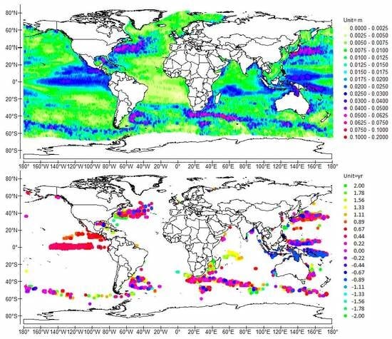
Figure 1.
Normalized cross-wavelet power (top) and coherence phase (bottom) of Sea Surface Height (SSH) scale-averaged over 8–16 months (1-year average period), time-averaged over 1992–2009 to reduce the noise because the sensitivity of the altimeter measurements decreases as latitude increases, gridded with a 1 × 1° resolution. Time elapses from the bottom to the top of the legend. The most significant values of the phase, which are associated with the highest values of the normalized cross-wavelet power, are the last drawn (the corresponding disks overlap with underlying discs). Data are provided by the French CNES (Centre National d’Etudes Spatiales): www.aviso.oceanobs.com.

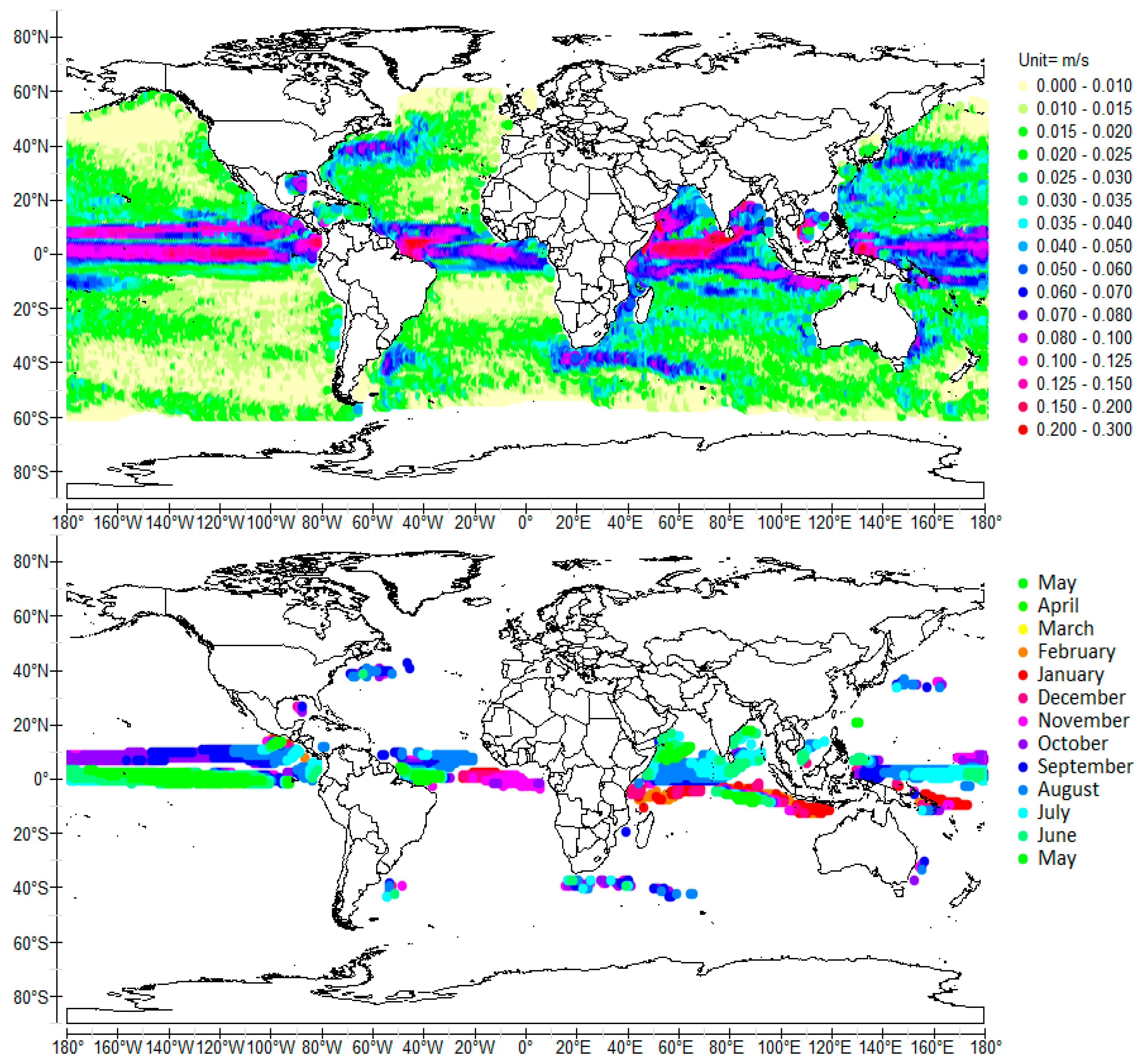
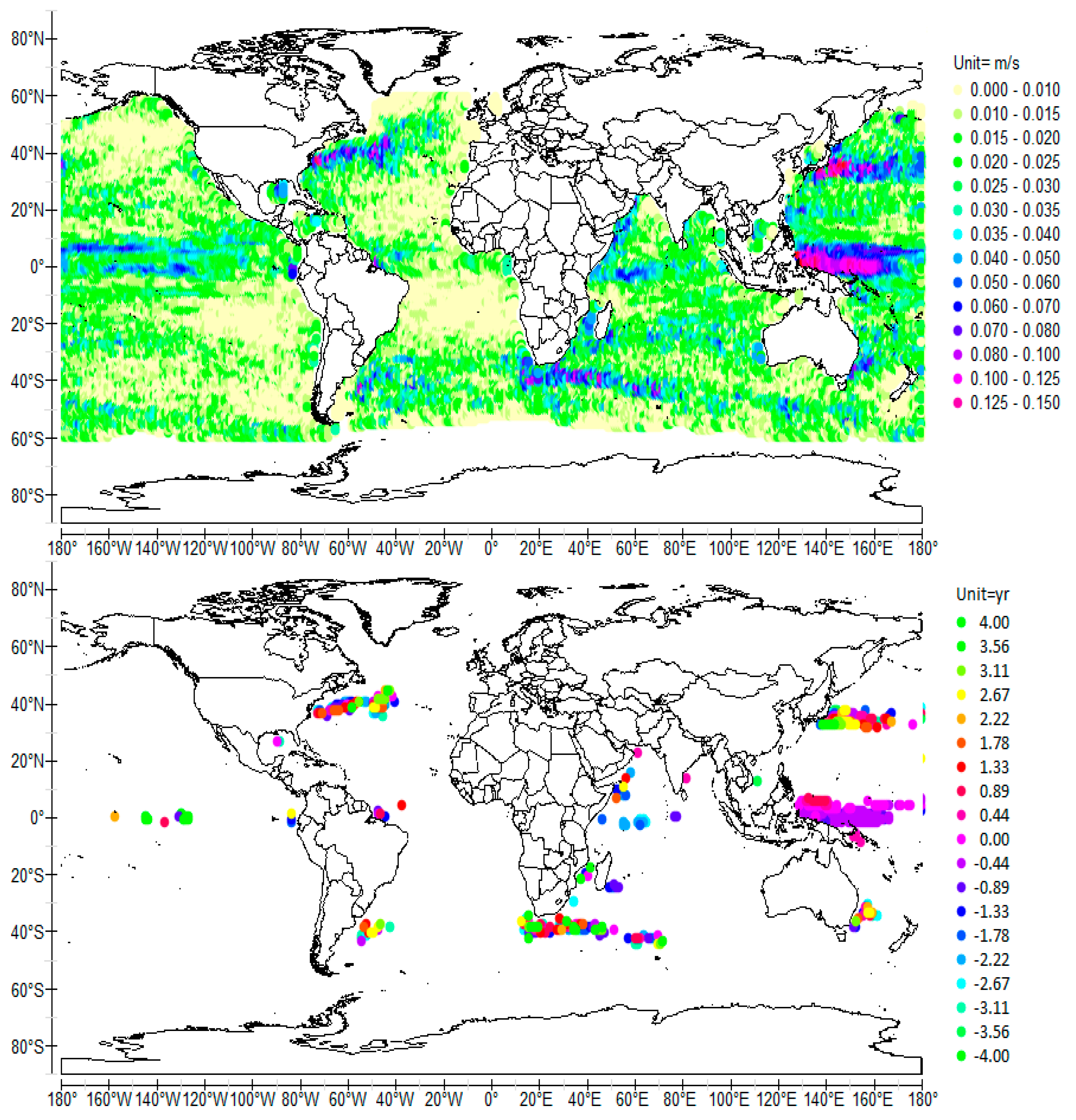
Figure 2.
Normalized cross-wavelet power (top) and coherence phase (bottom) of the signed magnitude ±v of Surface Current Velocity (SCV) scale-averaged over 8–16 months (1-year average period), time-averaged over 1992–2009, gridded with a 1 × 1° resolution. The phase refers to the time when the modulated current velocity reaches its maximum to the east. The maximum velocity to the west is reached T/2 later. Data are provided by the NOAA (National Oceanic and Atmospheric Administration): www.oscar.noaa.gov/datadisplay/datadownload.htm.

Figure 3.
Normalized cross-wavelet power (top) and coherence phase (bottom) of SSH scale-averaged over 5–7 months (6-month average period), time-averaged over 1992–2009. The same conventions as in Figure 1 are used.
Figure 3.
Normalized cross-wavelet power (top) and coherence phase (bottom) of SSH scale-averaged over 5–7 months (6-month average period), time-averaged over 1992–2009. The same conventions as in Figure 1 are used.
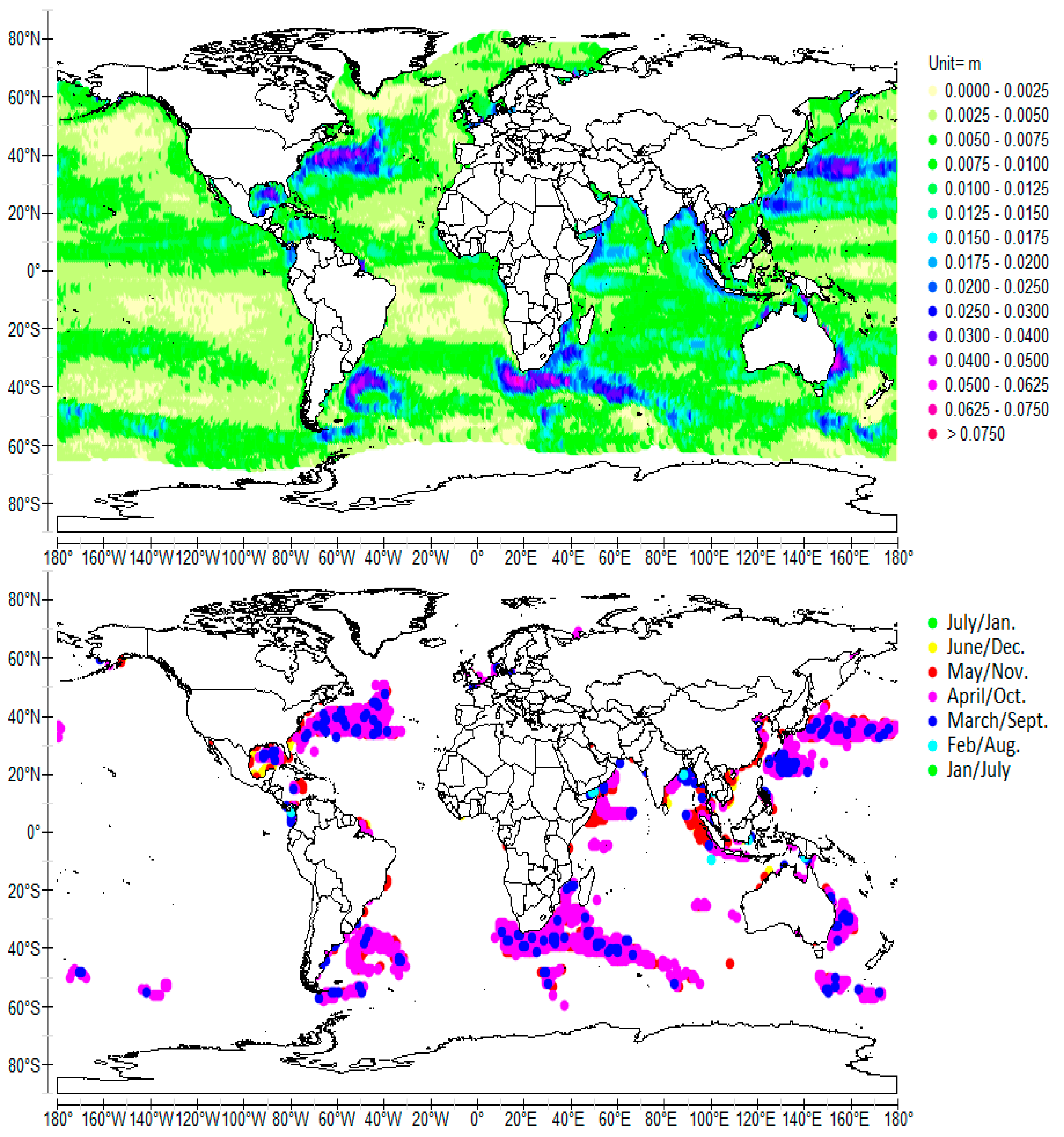
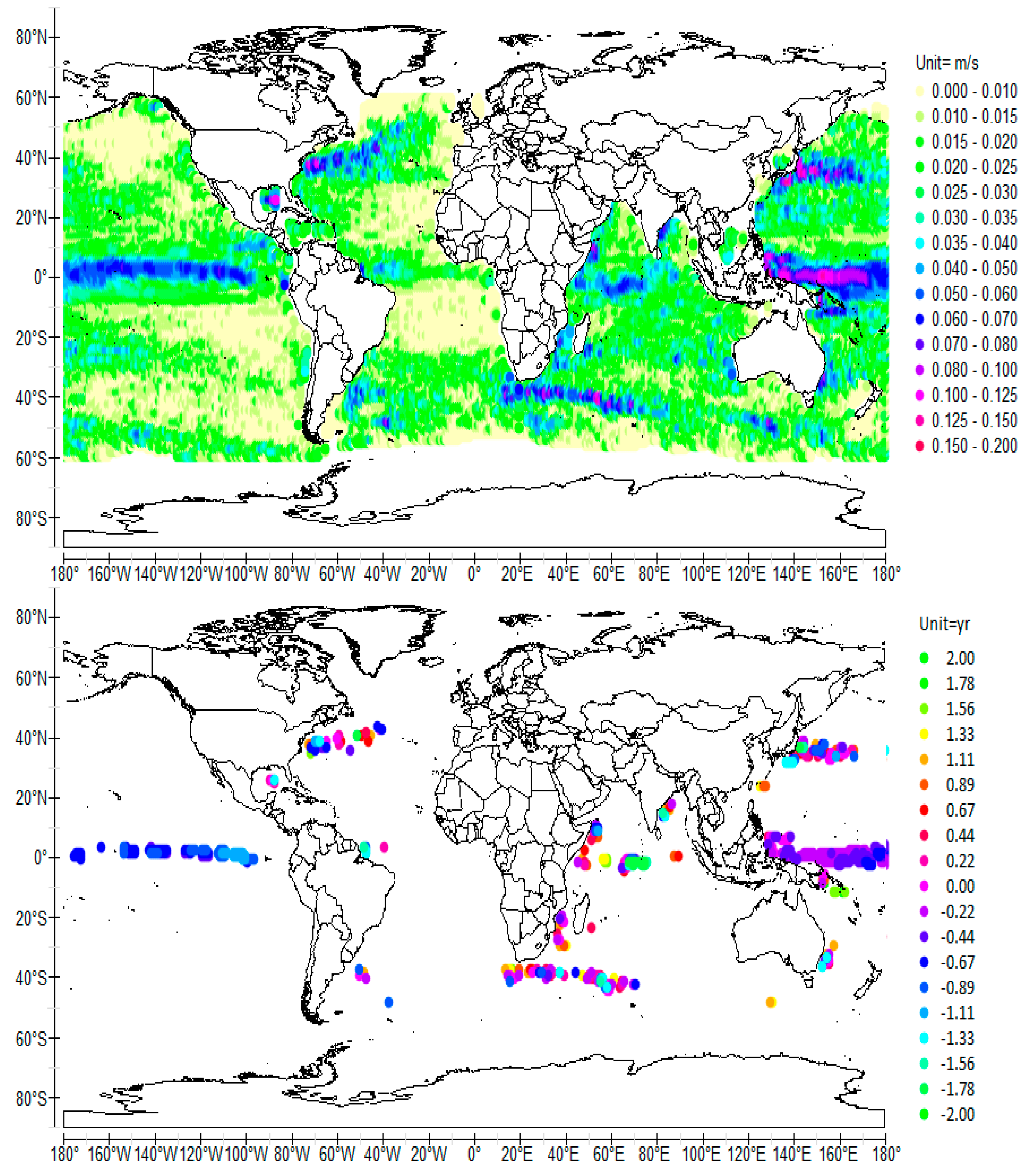
Figure 4.
Normalized cross-wavelet power (top) and coherence phase (bottom) of the signed magnitude ±v of SCV scale-averaged over 5–7 months (6-month average period), time-averaged over 1992–2009.
Figure 4.
Normalized cross-wavelet power (top) and coherence phase (bottom) of the signed magnitude ±v of SCV scale-averaged over 5–7 months (6-month average period), time-averaged over 1992–2009.
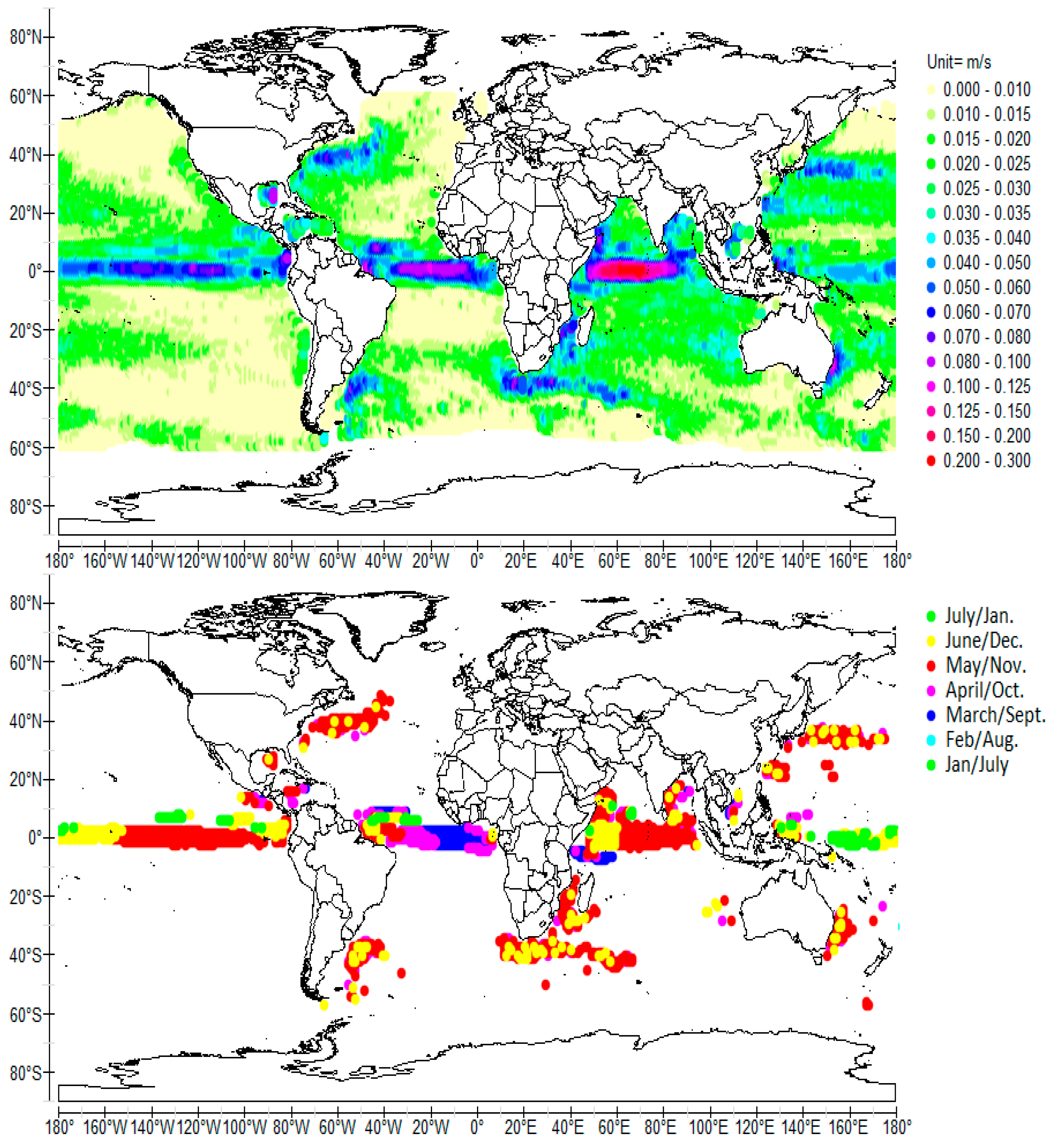
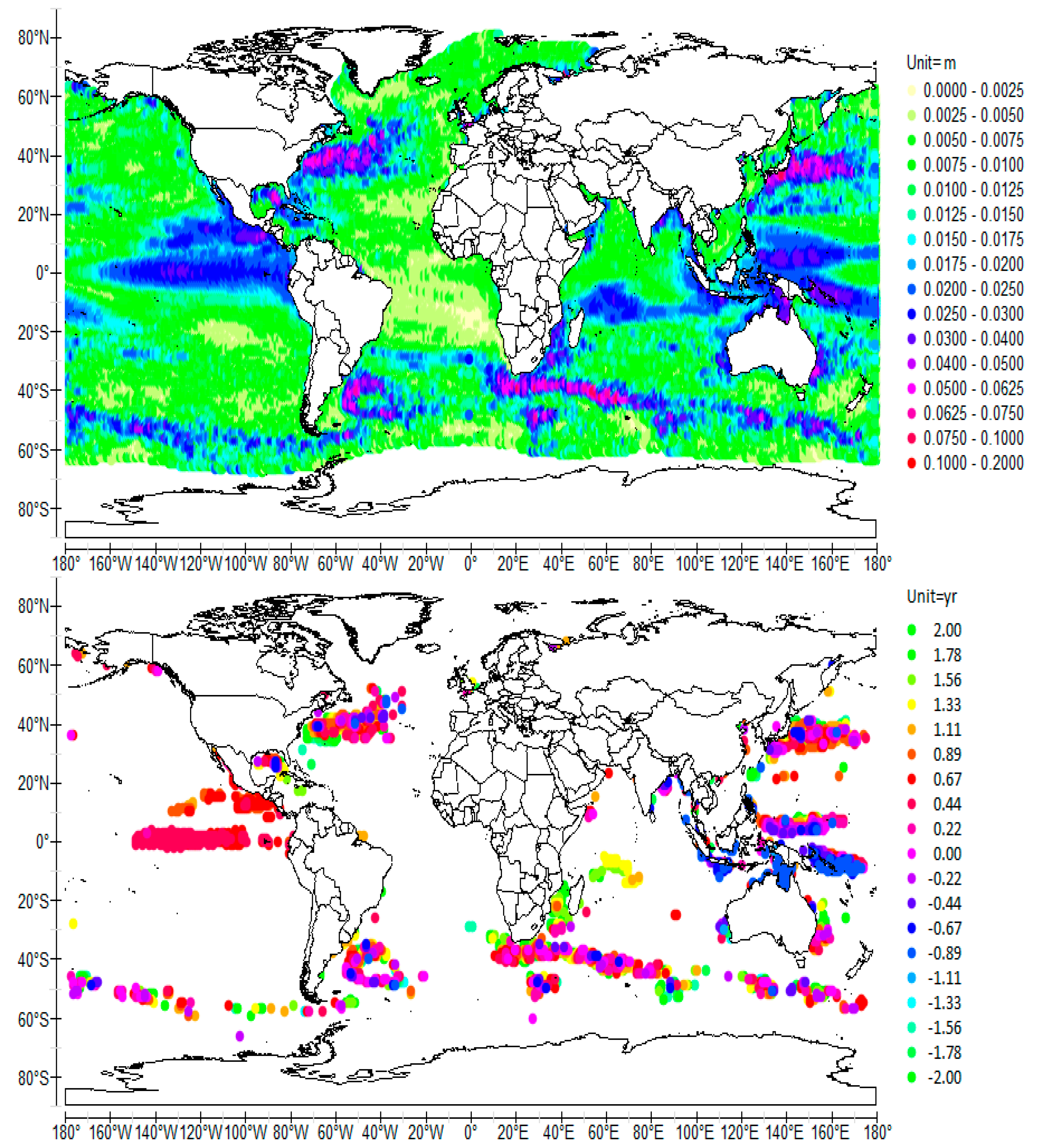
Figure 5.
Normalized cross-wavelet power (top) and coherence phase (bottom) of SSH and –SOI (used as the temporal reference) scale-averaged over 3.5–4.5 years (4-year average period), time-averaged over 1992–2009. –SOI, the opposite of the Southern Oscillation Index (SOI), turns out to be nearly in phase with SSH, the signed magnitude ±v of SCV at 4, 8 and longer periods across much of the oceans. So, the use of –SOI instead of SOI makes easier the interpretation of the coherence phase. The central value of the phase (shift = 0 year) corresponds to 03/2002 (or 03/2006, …). The monthly SOI is provided by the National Centre for Atmospheric Research: http://www.cgd.ucar.edu/cas/catalog/climind/soi.html.

Figure 6.
Normalized cross-wavelet power (top) and coherence phase (bottom) of the signed magnitude ±v of SCV and –SOI (used as the temporal reference) scale-averaged over 3.5–4.5 years (4-year average period), time-averaged over 1992–2009.
Figure 6.
Normalized cross-wavelet power (top) and coherence phase (bottom) of the signed magnitude ±v of SCV and –SOI (used as the temporal reference) scale-averaged over 3.5–4.5 years (4-year average period), time-averaged over 1992–2009.

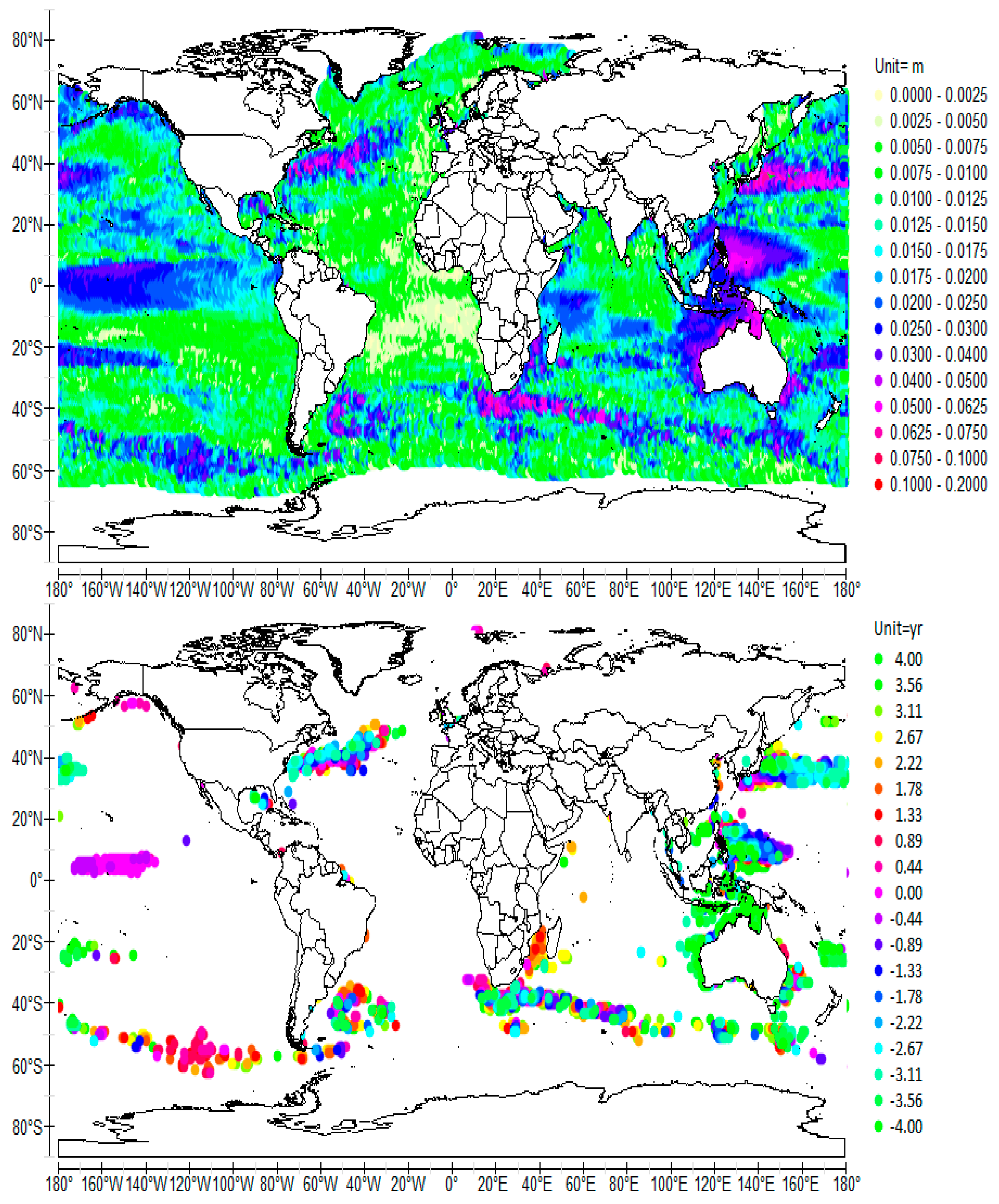
Figure 7.
Normalized cross-wavelet power (top) and coherence phase (bottom) of SSH and –SOI (used as the temporal reference) scale-averaged over 7.5–8.5 years (8-year average period), time-averaged over 1992–2009. The central value of the phase (shift = 0 year) corresponds to 04/2004 (or 04/2012 …).

Figure 8.
Normalized cross-wavelet power (top) and coherence phase (bottom) of the signed magnitude ±v of SCV and –SOI (used as the temporal reference) scale-averaged over 7.5–8.5 years (8-year average period), time-averaged over 1992–2009.
Figure 8.
Normalized cross-wavelet power (top) and coherence phase (bottom) of the signed magnitude ±v of SCV and –SOI (used as the temporal reference) scale-averaged over 7.5–8.5 years (8-year average period), time-averaged over 1992–2009.

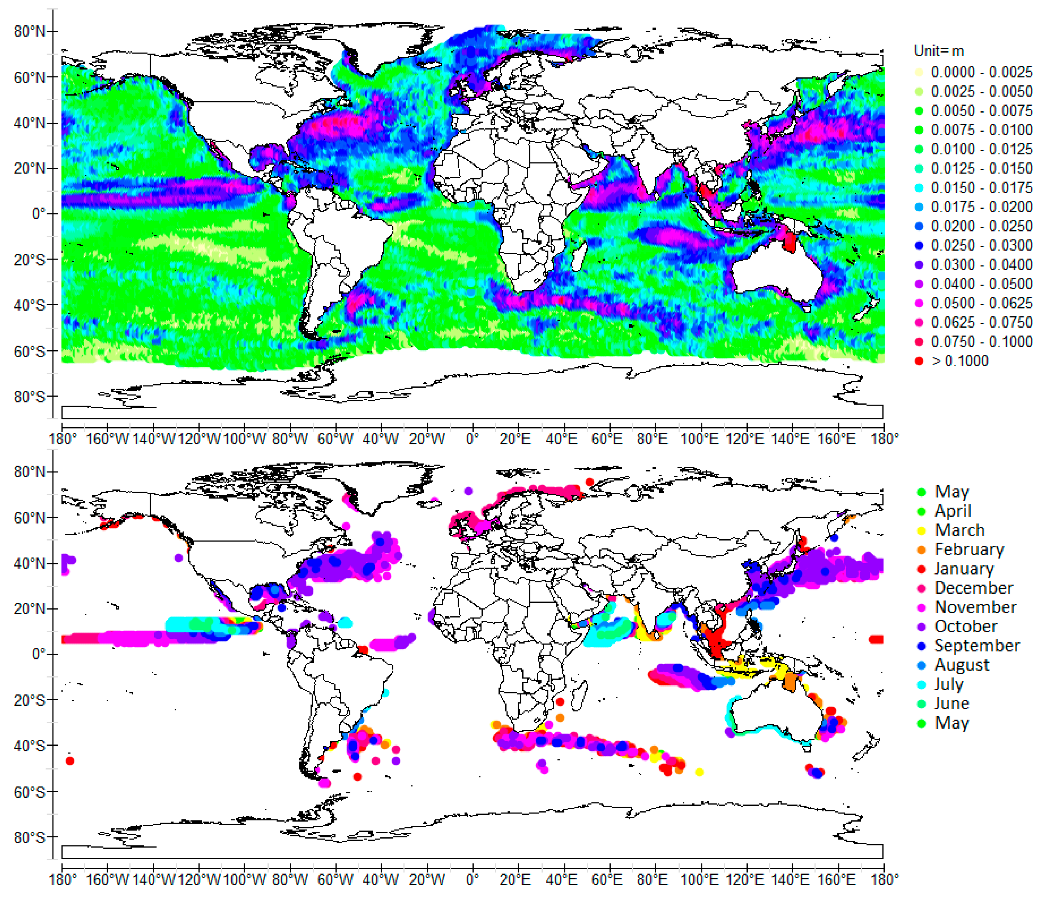
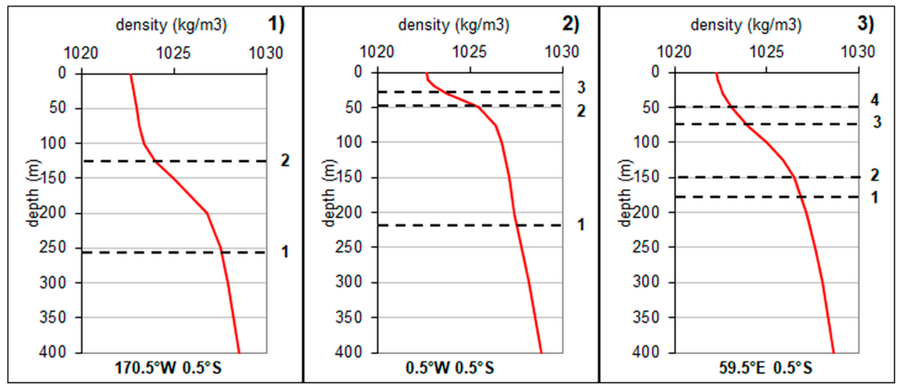
Figure 9.
Profiles of density considered as representative of equatorial oceans to determine the depth of the interfaces associated with normal modes for the Pacific (1), the Atlantic (2) and the Indian (3) Oceans. Interfaces associated with the first baroclinic modes are determined so that phase speeds are close to those observed, that is, 2.8, 2.35 and 2.3 m/s, respectively. Interfaces associated with the highest modes are positioned at the top of the pycnoclines: the lowest phase speeds allow explaining satisfactorily the resonance of 4- and 8-year period RFWs in the Indian and Atlantic oceans, respectively (one-eighth of the speed corresponding to the first mode). However, the resonance of a 4-year period RFW in the Atlantic and 1- and 2-year period RFWs in the Indian oceans that contribute to the Indian Ocean Dipole (IOD) suggests the existence of intermediate interfaces located within the pycnocline (their location is approximate). Data are provided by the NOAA (National Oceanic and Atmospheric Administration): http://iridl.ldeo.columbia.edu/expert/SOURCES/LEVITUS94/oceanviews2.html.

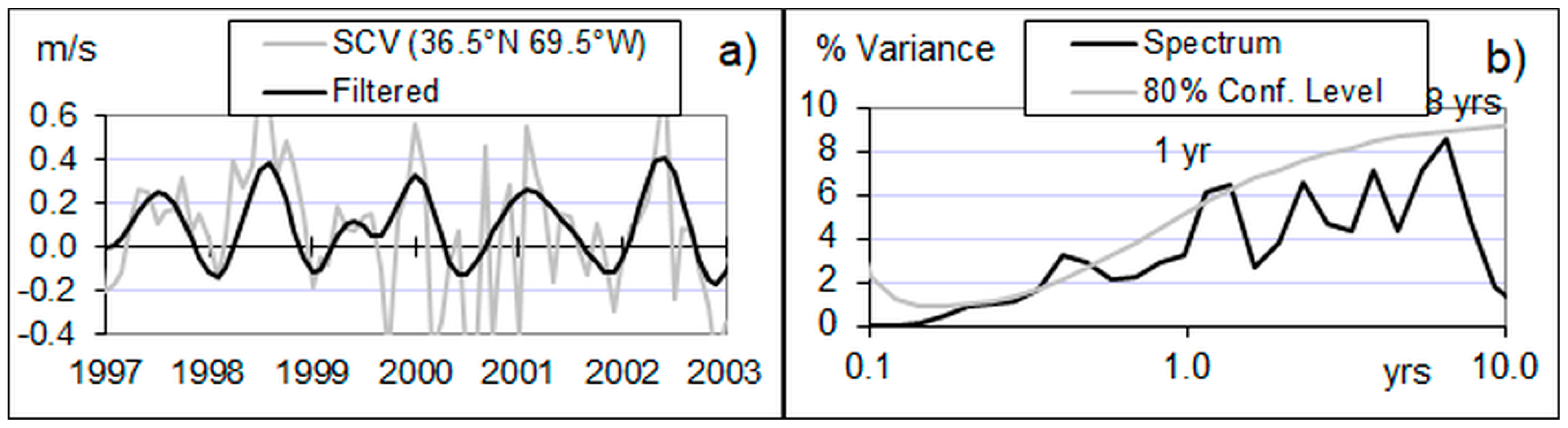
Figure 10.
(a) SCV (eastward) unfiltered and filtered with a bandpass filter within the 8–16 month band; (b) Fourier power spectrum of SCV from 1992 to 2009 and confidence spectrum assuming a red-noise with a lag-1 autocorrelation α = 0.46.
Figure 10.
(a) SCV (eastward) unfiltered and filtered with a bandpass filter within the 8–16 month band; (b) Fourier power spectrum of SCV from 1992 to 2009 and confidence spectrum assuming a red-noise with a lag-1 autocorrelation α = 0.46.

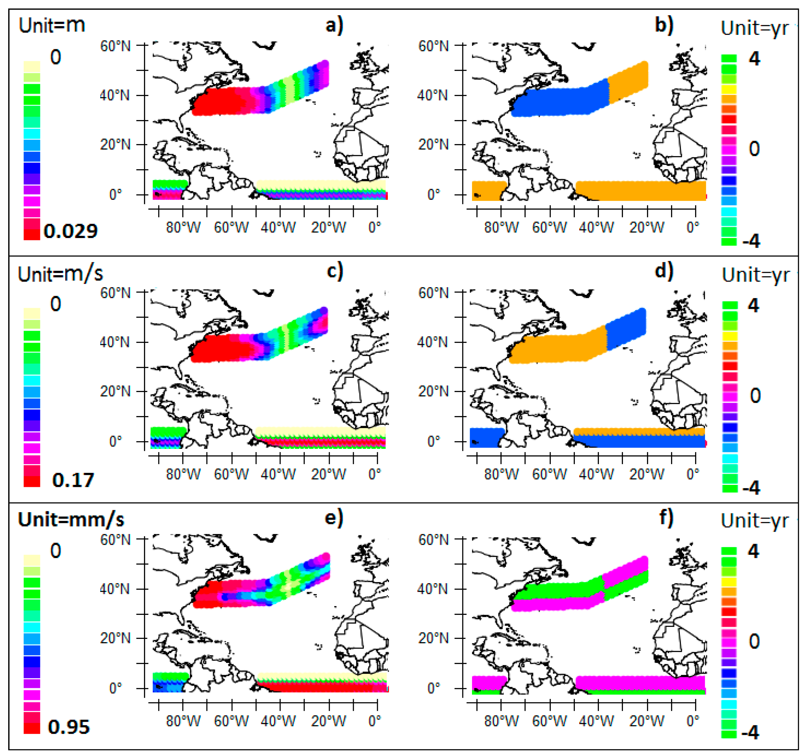
Figure 11.
The solution of the equations of motion in the North Atlantic for the 8-year period Resonantly Forced Waves (RFW) supposing the wind-driven circulation velocity is 0.038 m/s [19]. Represented are the wavelet power (on the left) and the coherence phase (on the right) of the perturbation η of SSH (a,b), the zonal modulated current velocity (c,d), the phase refers to the modulated currents flowing eastward (the wind-driven circulation is ignored) and the meridional modulated current velocity (e,f) (the phase refers to the modulated currents flowing northward). Only the equatorial waves are represented in the tropical ocean: the interface associated with the vertical baroclinic mode is at the top of the pycnocline (the highest mode n = 3 for the Atlantic). First baroclinic mode Rossby waves occur at mid-latitudes: the mean depth of the thermocline is supposed to be 60 m, the density of the mixed layer 1025 kg/m3. The changes in density are small because excess salinity where evaporation occurs is the most important, which is to say the neighboring latitudes of 10° N or S, are offset by the thermal expansion of warm waters. Around the gyres the approximation is made that where and are the density of the upper and the lower layer, respectively. The ratio μ = η/∆h is taken to 0.0025 (∆h is the amplitude of the vertical motion of the interface). The length of partial sums of Fourier series is 24 versus both the longitude and the time. The decay rate of friction r = αω is 2.5 × 10⁻⁹ s−1 (α = 0.1): ω = 2π⁄T, T = 8 years for Rossby waves and 1.7 × 10⁻⁹ s−1 (α = 0.017), T = 0.5 year for Kelvin waves. The time of transfer of warm water from the equator to mid-latitudes is neglected, being small in comparison with the period.


Table 1.
Phase speed for the first four baroclinic modes. It is supposed eigenvectors vanish around 1750 m [15].
Table 1.
Phase speed for the first four baroclinic modes. It is supposed eigenvectors vanish around 1750 m [15].
| Location | Depth (m) | Density (kg/m3) | 1st (m/s) | 2nd (m/s) | 3rd (m/s) | 4th (m/s) |
|---|---|---|---|---|---|---|
| Pacific 170.5 W 0.5 S | 0–125 125–255 255–1750 | 1023.03 1025.52 1031.58 | 2.79 | 0.99 | ||
| Atlantic 0.5 W 0.5 S | 0–30 30–50 50–220 220–1750 | 1022.82 1023.74 1026.63 1031.58 | 2.33 | 0.81 | 0.28 | |
| Indian 59.5 E 0.5 S | 0–50 50–75 75–150 150–180 180–1750 | 1022.48 1023.08 1024.98 1026.49 1031.45 | 2.33 | 0.98 | 0.55 | 0.28 |
Table 2.
The apparent half-wavelength of the 8-year period Rossby waves, the apparent phase velocity of Rossby waves and the speed of the wind-driven circulation of the five subtropical gyres.
Table 2.
The apparent half-wavelength of the 8-year period Rossby waves, the apparent phase velocity of Rossby waves and the speed of the wind-driven circulation of the five subtropical gyres.
| North Atlantic | South Atlantic | North Pacific | South Pacific | South Indian | |
|---|---|---|---|---|---|
| Apparent 1/2 wavelength (km) | 3400 | 2700 | 4900 | 2300 | 5500 |
| Apparent velocity (m/s) | 0.027 | 0.022 | 0.039 | 0.018 | 0.044 |
| Speed of wind-driven circulation (m/s) | 0.038 | 0.033 | 0.055 | 0.028 | 0.055 |
© 2018 by the author. Licensee MDPI, Basel, Switzerland. This article is an open access article distributed under the terms and conditions of the Creative Commons Attribution (CC BY) license (http://creativecommons.org/licenses/by/4.0/).
Share and Cite
MDPI and ACS Style
Pinault, J.-L. Resonantly Forced Baroclinic Waves in the Oceans: Subharmonic Modes. J. Mar. Sci. Eng. 2018, 6, 78. https://doi.org/10.3390/jmse6030078
AMA Style
Pinault J-L. Resonantly Forced Baroclinic Waves in the Oceans: Subharmonic Modes. Journal of Marine Science and Engineering. 2018; 6(3):78. https://doi.org/10.3390/jmse6030078
Chicago/Turabian StylePinault, Jean-Louis. 2018. "Resonantly Forced Baroclinic Waves in the Oceans: Subharmonic Modes" Journal of Marine Science and Engineering 6, no. 3: 78. https://doi.org/10.3390/jmse6030078
Note that from the first issue of 2016, this journal uses article numbers instead of page numbers. See further details here.