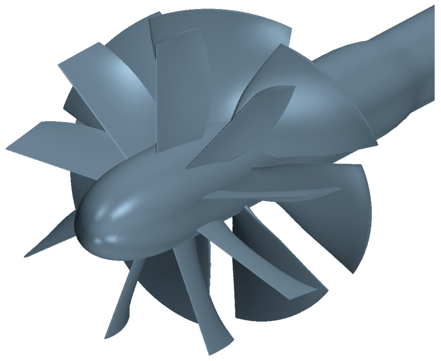
Figure 1.
The geometric model of the seven-bladed rotor and the nine-bladed pre-swirl stator. The stator blades are connected to the shroud surface without clearance. The shroud surface is omitted.
Figure 1.
The geometric model of the seven-bladed rotor and the nine-bladed pre-swirl stator. The stator blades are connected to the shroud surface without clearance. The shroud surface is omitted.
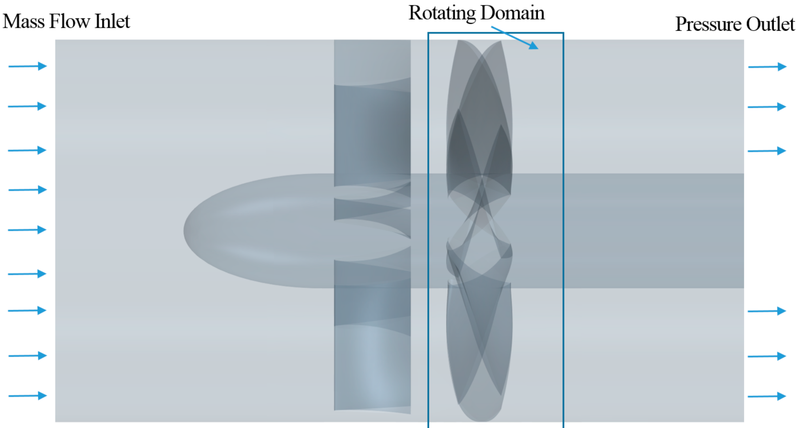
Figure 2.
The computational domain for the axial-flow pump. The domain is a circular cylinder bounded by the shroud surface, 16 times the shroud diameter in length. The rotor is located at the longitudinal center of the domain, while the stator is located upstream of the rotor.
Figure 2.
The computational domain for the axial-flow pump. The domain is a circular cylinder bounded by the shroud surface, 16 times the shroud diameter in length. The rotor is located at the longitudinal center of the domain, while the stator is located upstream of the rotor.
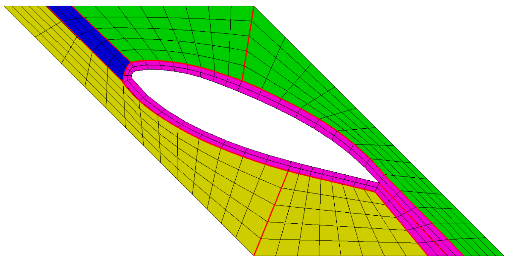
Figure 3.
Grid topology around rotor blade sections.
Figure 3.
Grid topology around rotor blade sections.
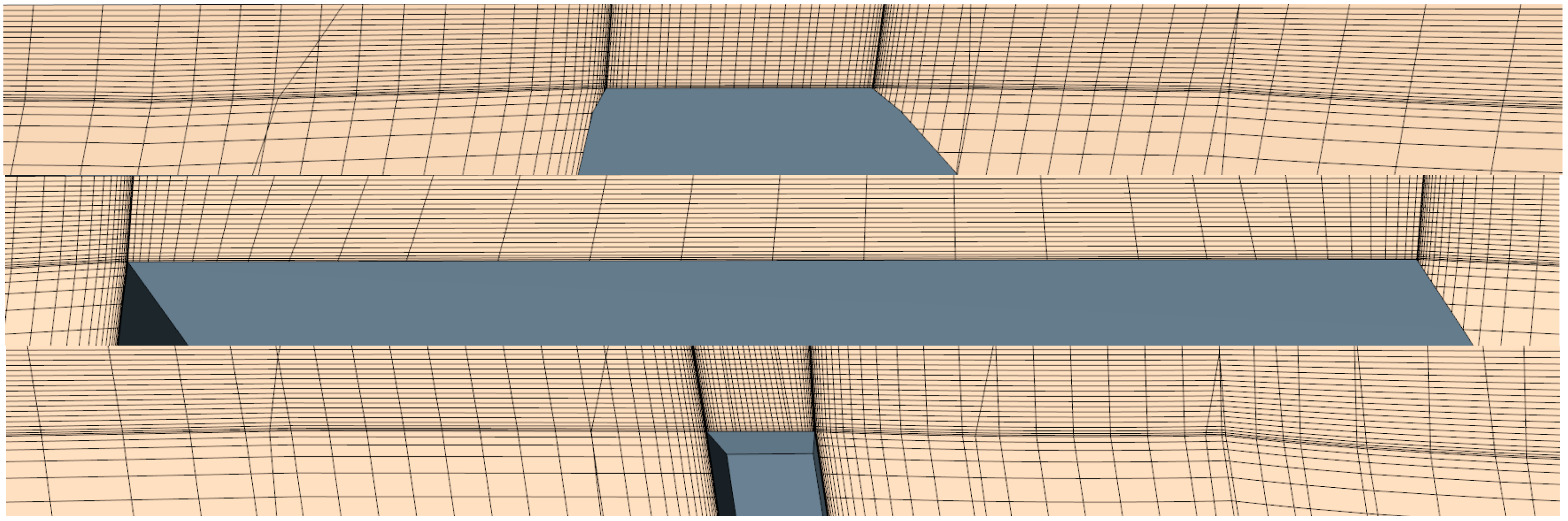
Figure 4.
The grid structure in the tip clearance of a rotor. The sections perpendicular to the nose-tail chord of the tip are shown at 10% (top), 50% (middle), and 90% (bottom) chord length.
Figure 4.
The grid structure in the tip clearance of a rotor. The sections perpendicular to the nose-tail chord of the tip are shown at 10% (top), 50% (middle), and 90% (bottom) chord length.
Figure 5.
The surface grids for rotor and stator blades.
Figure 5.
The surface grids for rotor and stator blades.
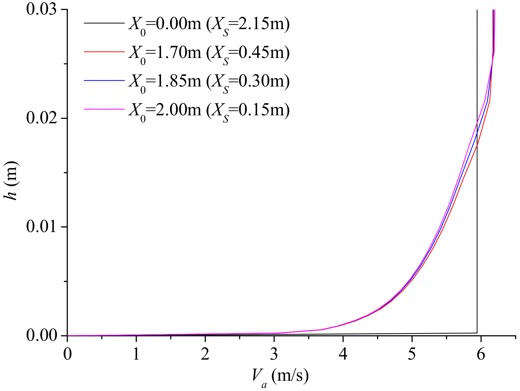
Figure 6.
Simulated axial velocity profiles in shroud-surface boundary layer, where h is the normal distance from the shroud surface, X0 is the distance measured from the inlet, and XS is the distance to the nose of shaft cap.
Figure 6.
Simulated axial velocity profiles in shroud-surface boundary layer, where h is the normal distance from the shroud surface, X0 is the distance measured from the inlet, and XS is the distance to the nose of shaft cap.
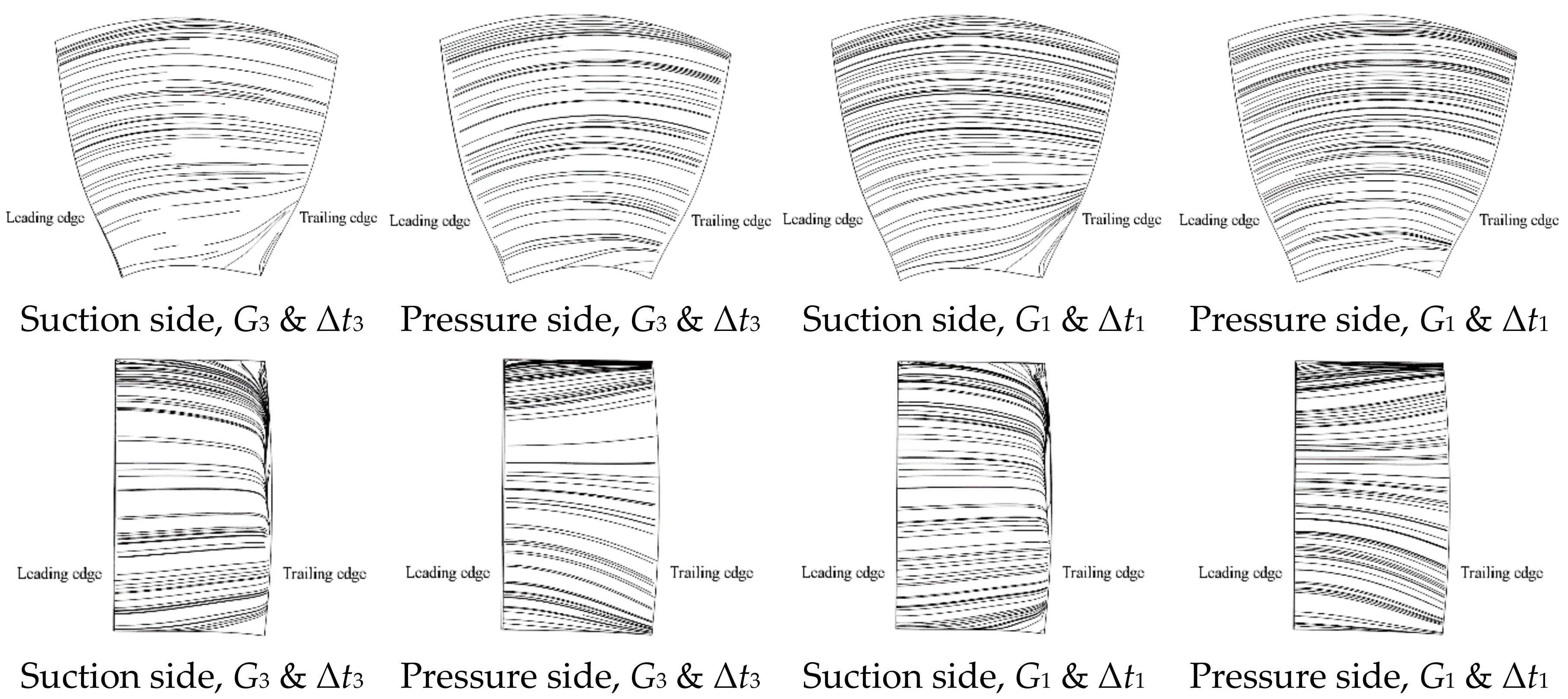
Figure 7.
Limiting streamlines on rotor (top row) and stator (bottom row) blade surfaces, Q = 0.42 m3/s.
Figure 7.
Limiting streamlines on rotor (top row) and stator (bottom row) blade surfaces, Q = 0.42 m3/s.
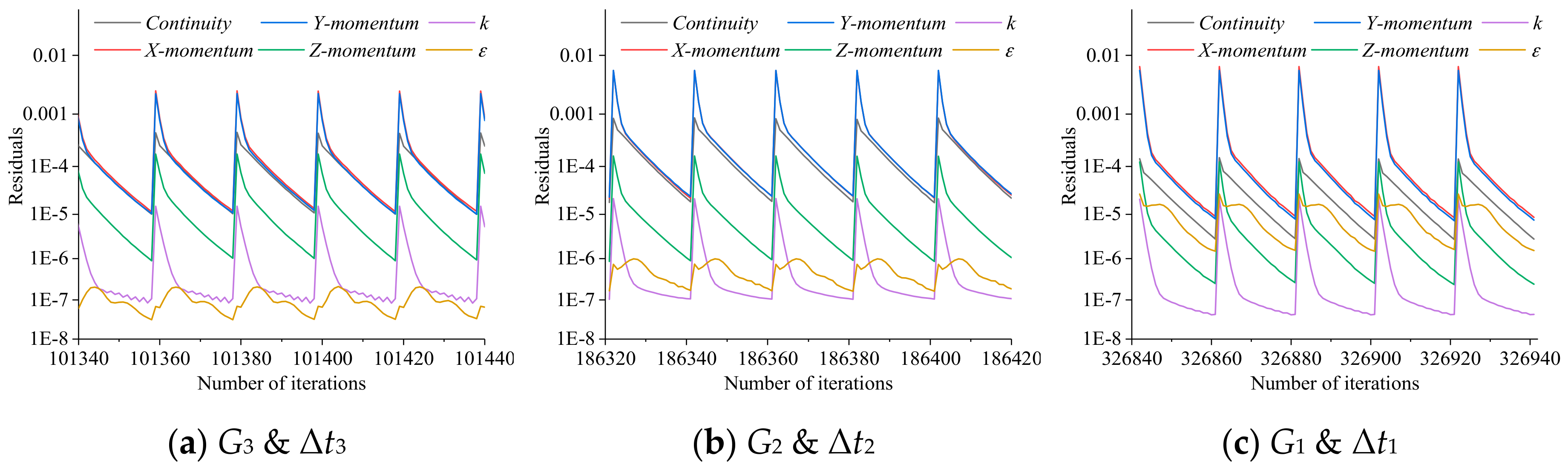
Figure 8.
Example of residuals in the last few time steps before convergence, Q = 0.42 m3/s.
Figure 8.
Example of residuals in the last few time steps before convergence, Q = 0.42 m3/s.
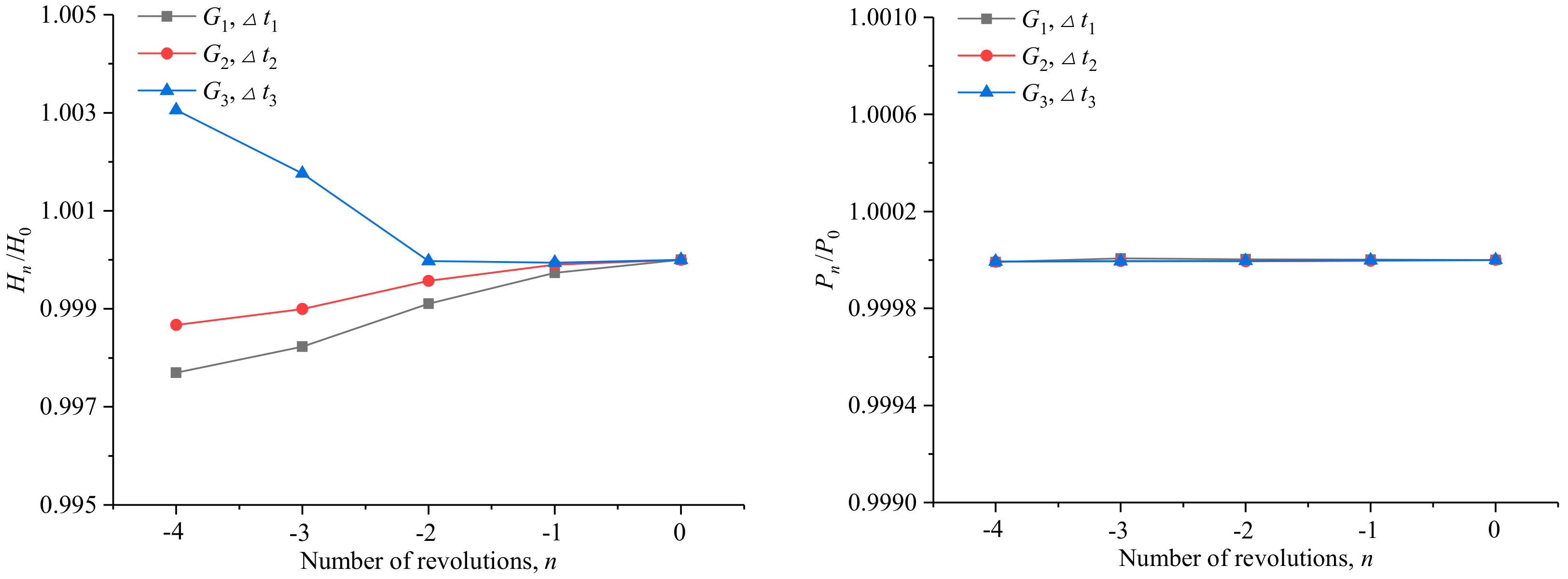
Figure 9.
The convergence history of the averaged head H (left) and power P (right) in the last five revolutions before convergence, Q = 0.42 m3/s. The abscissa, n, denotes the number of revolutions relative to the last revolution (n = 0). The ordinates Hn and Pn denote the head and power of the nth revolution, respectively.
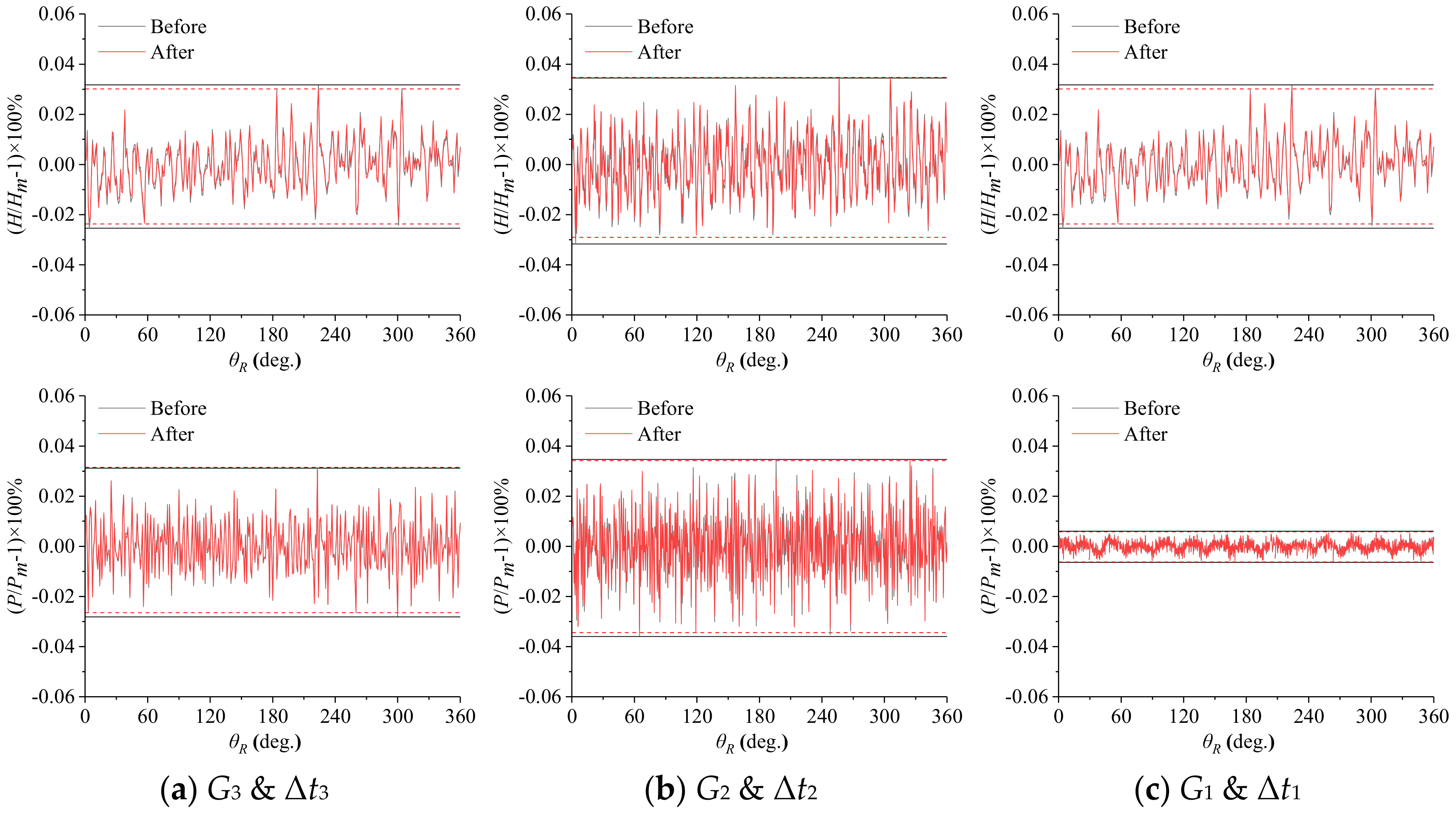
Figure 10.
Comparison of the unsteady head H (top row) and power P (bottom row) before (black lines) and after (red lines) removing the components arising from stator/rotor interaction. The abscissa, θR, denotes the angular position of a rotor blade. The head and power are expressed respectively in percents relative to Hm and Pm, the averages over a complete revolution. Q = 0.42 m3/s.
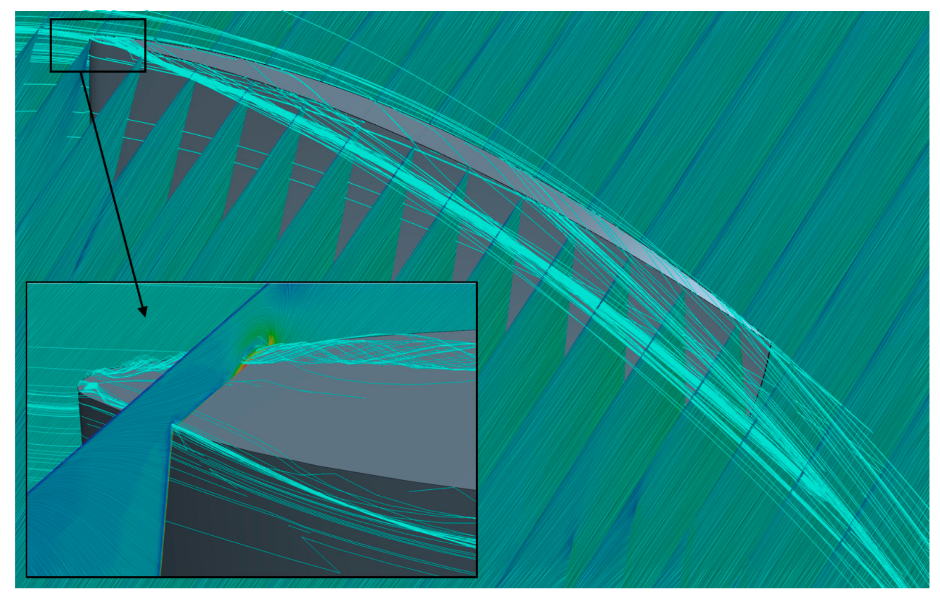
Figure 11.
The streamlines around a blade tip. Q = 0.42 m3/s.
Figure 11.
The streamlines around a blade tip. Q = 0.42 m3/s.
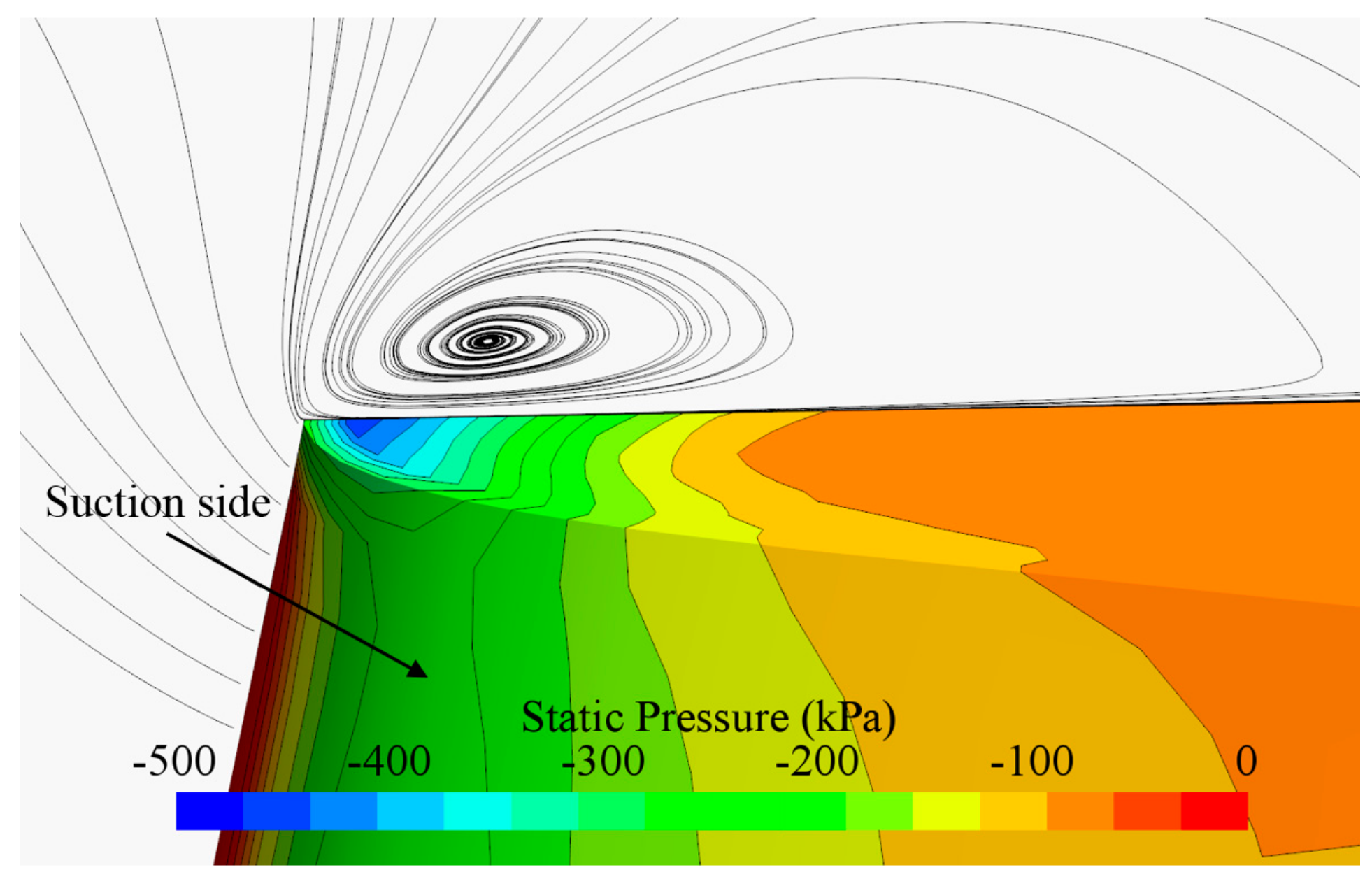
Figure 12.
Pressure contours on the tip surface and streamlines in the tip clearance. Q = 0.42 m3/s.
Figure 12.
Pressure contours on the tip surface and streamlines in the tip clearance. Q = 0.42 m3/s.
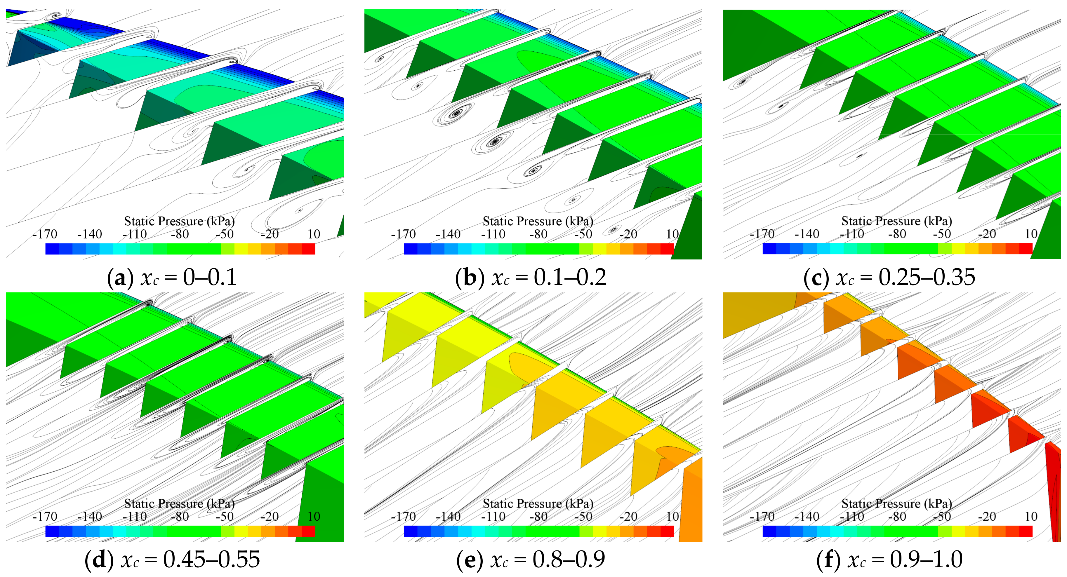
Figure 13.
The streamlines (colored by static pressures) in sections across the tip surface, where xc is the chordwise distance from the leading edge in fractions of the chord length. Q = 0.42 m3/s.
Figure 13.
The streamlines (colored by static pressures) in sections across the tip surface, where xc is the chordwise distance from the leading edge in fractions of the chord length. Q = 0.42 m3/s.
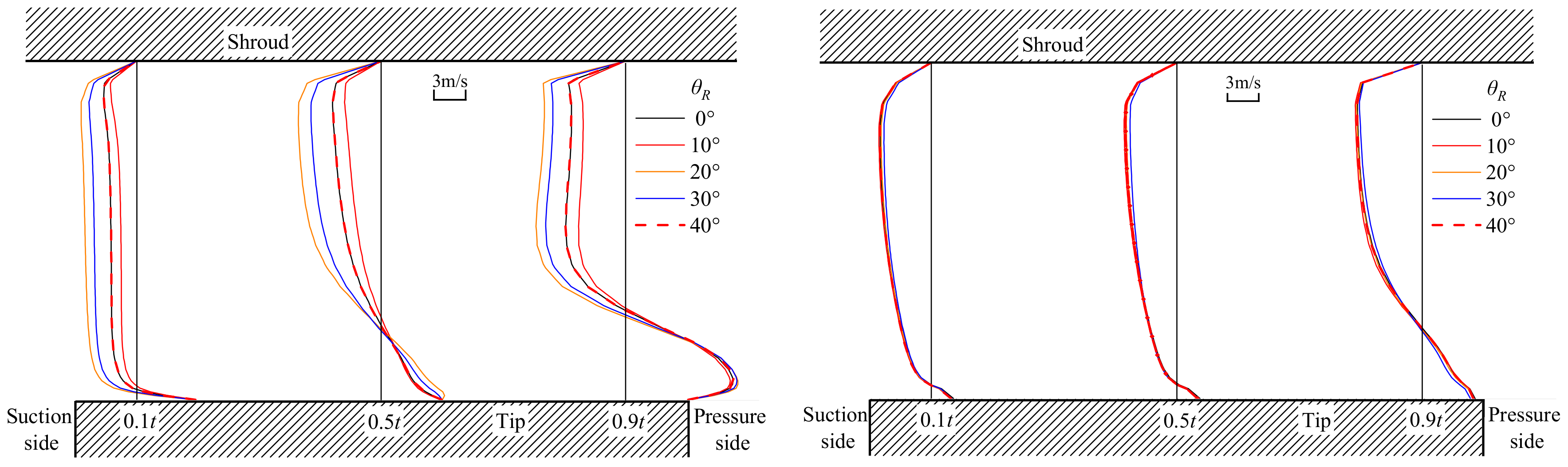
Figure 14.
In-plane absolute velocity profiles in the tip clearance at 10% (left) and 50% (right) chord length. The velocity profiles shown at five instantaneous positions of the rotor θR cover the angular spacing between adjacent stator blades. From suction side to pressure side, three sections are taken at 10%, 50% and 90% of the local thickness t, respectively. The velocity magnitude is zero at the vertical straight lines. The shroud is stationary. The rotor tip rotates from left to right. Q = 0.42 m3/s.
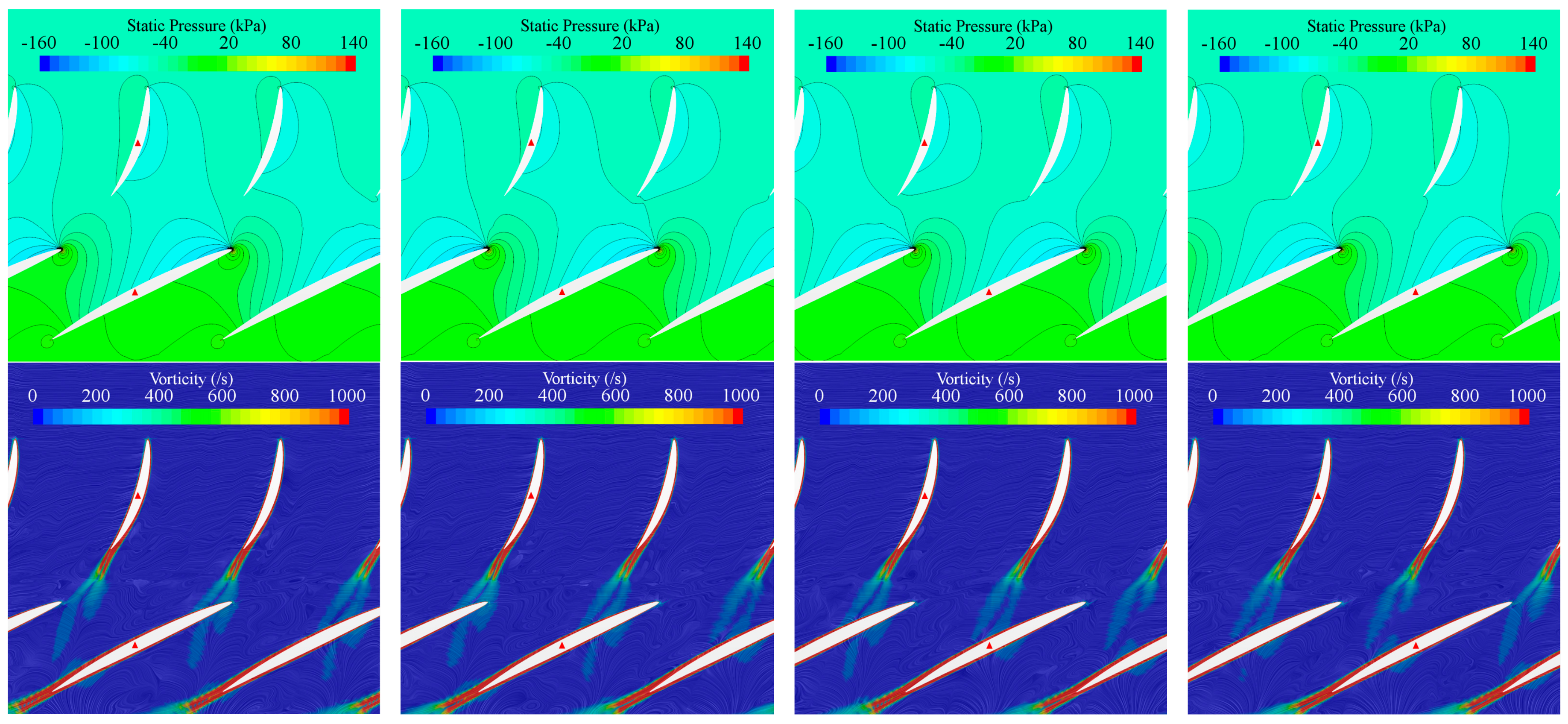
Figure 15.
The pressure (top row) and vorticity (bottom row) around stator and rotor blade sections at 0.7Rtip. The rotor blade angle θR = 0°, 10°, 20°, 30° (from left to right). Q = 0.42 m3/s.
Figure 15.
The pressure (top row) and vorticity (bottom row) around stator and rotor blade sections at 0.7Rtip. The rotor blade angle θR = 0°, 10°, 20°, 30° (from left to right). Q = 0.42 m3/s.
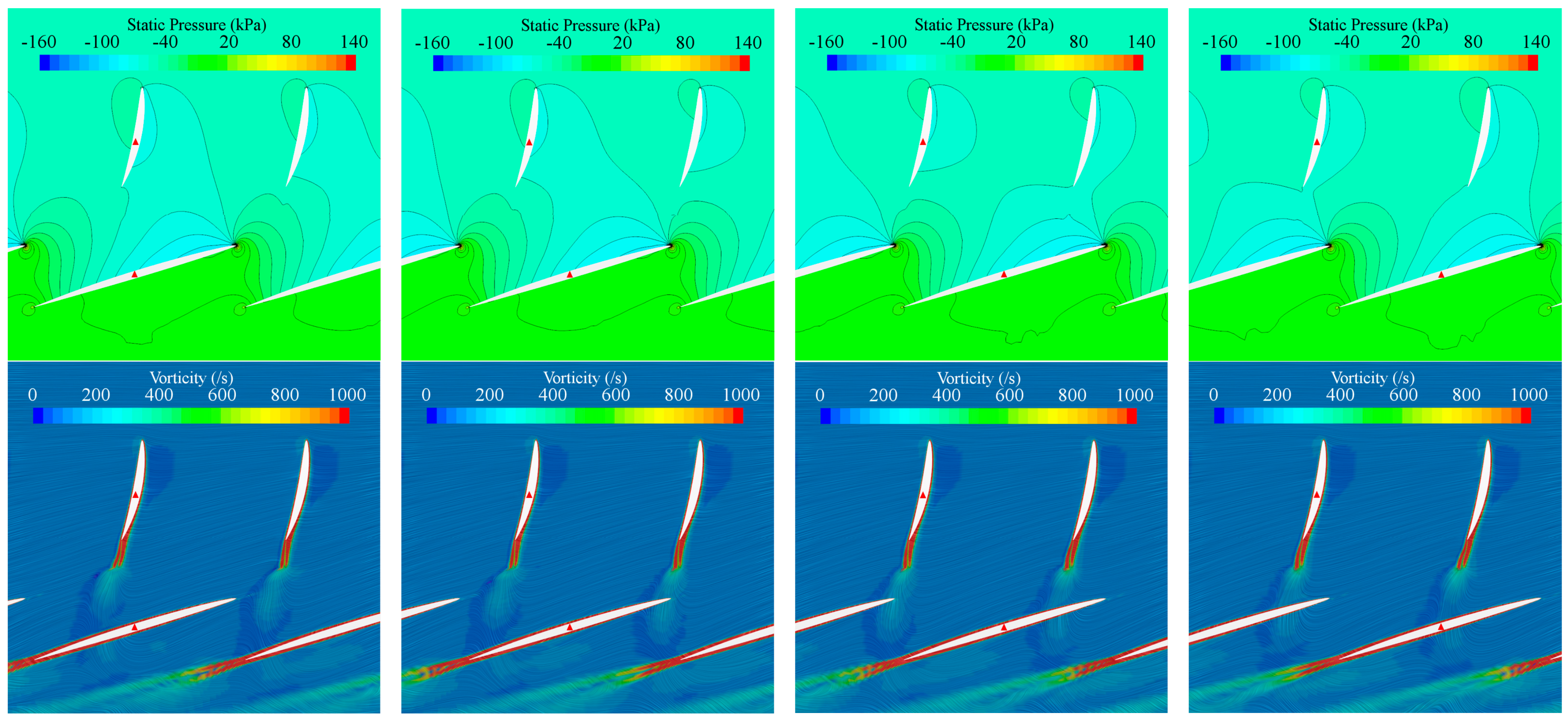
Figure 16.
The pressure (top row) and vorticity (bottom row) around stator and rotor blade sections at 0.95Rtip. The rotor blade angle θR = 0°, 10°, 20°, 30° (from left to right). Q = 0.42 m3/s.
Figure 16.
The pressure (top row) and vorticity (bottom row) around stator and rotor blade sections at 0.95Rtip. The rotor blade angle θR = 0°, 10°, 20°, 30° (from left to right). Q = 0.42 m3/s.
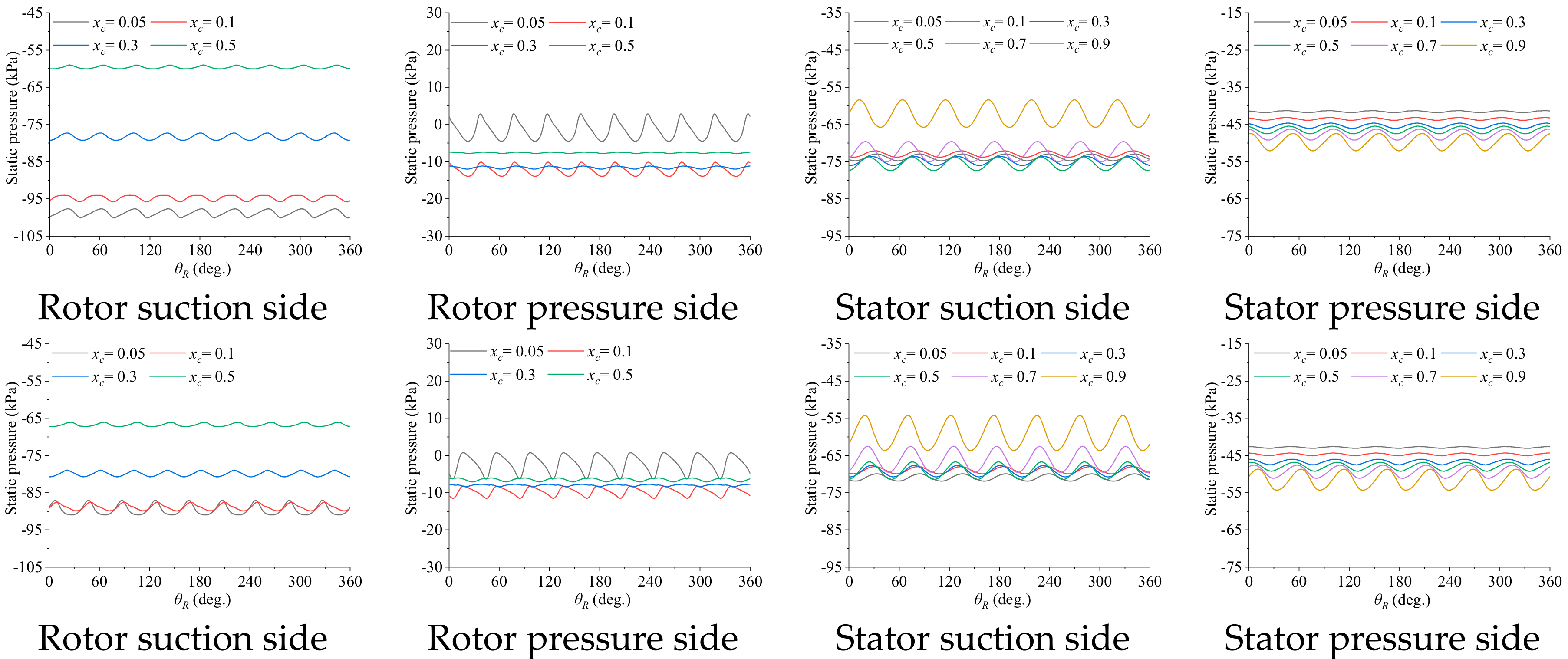
Figure 17.
Blade-surface pressure oscillations in a complete revolution of the rotor at 0.7Rtip (top row) and 0.95Rtip (bottom row). xc denotes the chordwise location from section nose in fractions of the chord length. θR denotes the angular position of a rotor blade. Q = 0.42 m3/s.
Figure 17.
Blade-surface pressure oscillations in a complete revolution of the rotor at 0.7Rtip (top row) and 0.95Rtip (bottom row). xc denotes the chordwise location from section nose in fractions of the chord length. θR denotes the angular position of a rotor blade. Q = 0.42 m3/s.
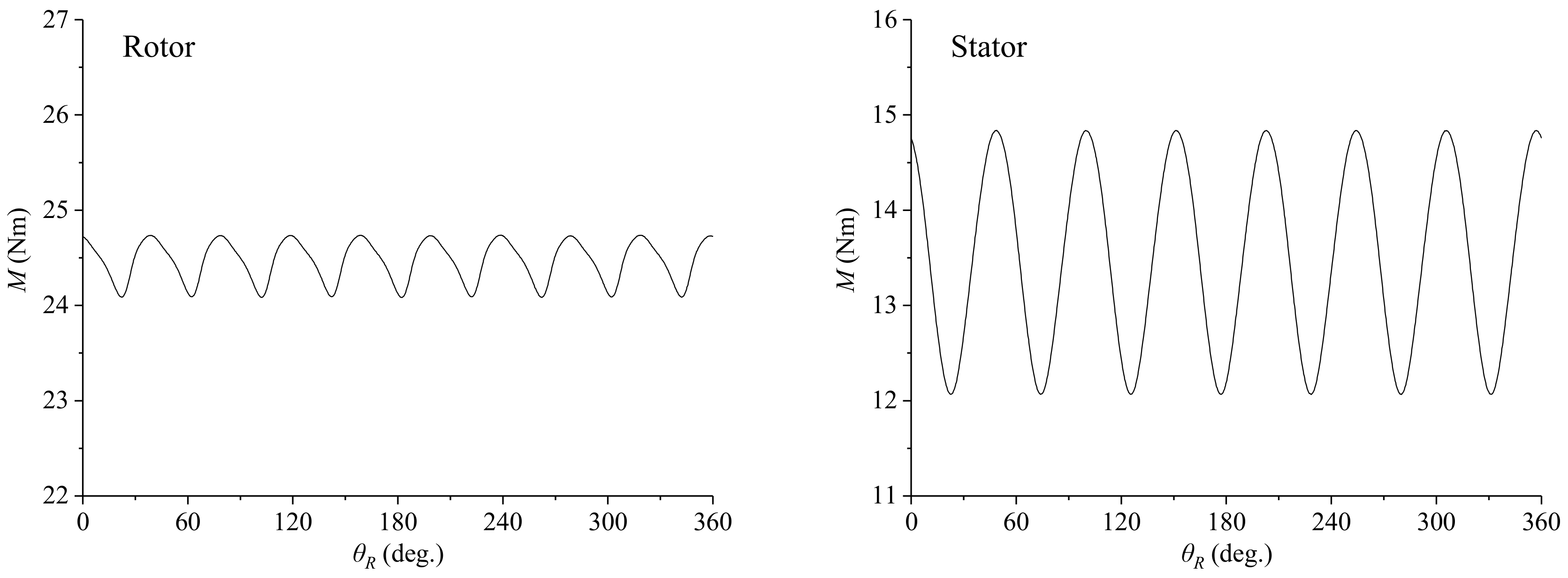
Figure 18.
Oscillations of the torques on a rotor blade (left) and a stator blade (right). θR denotes the angular position of the rotor blade. Q = 0.42 m3/s.
Figure 18.
Oscillations of the torques on a rotor blade (left) and a stator blade (right). θR denotes the angular position of the rotor blade. Q = 0.42 m3/s.
Table 1.
Key parameters of the computational grids.
Table 1.
Key parameters of the computational grids.
| Grid ID | Maximum Cell Size on Blade Surface (mm) | First-Layer Cell Height from Blade Surface (mm) | Number of Cells in Tip-Clearance | Total Number of Cells (Million) |
|---|
| Stator | Rotor | Stator | Rotor | Radial | Circumferential |
|---|
| G3 | 5 | 4 | 0.02 | 0.01 | 10 | 16 | 1.79 |
| G2 | 3.54 | 2.83 | 0.014 | 0.007 | 15 | 22 | 4.87 |
| G1 | 2.5 | 2 | 0.01 | 0.005 | 20 | 30 | 13.17 |
Table 2.
Range of the surface-averaged y+, Q = 0.35 m3/s–0.471 m3/s.
Table 2.
Range of the surface-averaged y+, Q = 0.35 m3/s–0.471 m3/s.
| Grid ID | Stator | Rotor | Tip Clearance |
|---|
| G3 | 3.2–4.2 | 1.9–2.3 | 5.7–5.8 |
| G2 | 2.3–3.0 | 1.4–1.6 | 4.7–4.8 |
| G1 | 1.7–2.3 | 1.0–1.3 | 3.3–3.4 |
Table 3.
Comparison of simulation results and experimental data [
25] for the axial-flow pump.
Table 3.
Comparison of simulation results and experimental data [
25] for the axial-flow pump.
| Q (m3/s) | Grid, Time-Step Size | Simulation Result S | Experimental Data D | Comparison Error E (%D) |
|---|
| H (m) | P(kW) | H (m) | P (kW) | H | P |
|---|
| 0.35 | G3, Δt3 | 7.320 | 29.473 | 7.450 | 31.341 | −1.47 | −5.96 |
| G2, Δt2 | 7.373 | 29.541 | −1.04 | −5.74 |
| G1, Δt1 | 7.406 | 29.584 | −0.59 | −5.61 |
| 0.42 | G3, Δt3 | 5.221 | 25.343 | 5.400 | 25.957 | −3.31 | −2.36 |
| G2, Δt2 | 5.247 | 25.414 | −2.83 | −2.09 |
| G1, Δt1 | 5.267 | 25.473 | −2.45 | −1.87 |
| 0.471 | G3, Δt3 | 3.476 | 20.341 | 3.600 | 20.305 | −3.44 | 0.18 |
| G2, Δt2 | 3.521 | 20.456 | −2.18 | 0.75 |
| G1, Δt1 | 3.546 | 20.513 | −1.49 | 1.02 |
Table 4.
Iteration uncertainties in the simulations.
Table 4.
Iteration uncertainties in the simulations.
| Q (m3/s) | | G3, Δt3 (%S) | G2, Δt2 (%S) | G1, Δt1 (%S) |
|---|
| 0.35 | H | 0.03 | 0.02 | 0.02 |
| 0.42 | 0.03 | 0.03 | 0.01 |
| 0.471 | 0.04 | 0.04 | 0.01 |
| 0.35 | P | 0.03 | 0.02 | 0.01 |
| 0.42 | 0.03 | 0.03 | 0.01 |
| 0.471 | 0.04 | 0.04 | 0.01 |
Table 5.
Results of the numerical uncertainties at different flow rates.
Table 5.
Results of the numerical uncertainties at different flow rates.
| Q (m3/s) | | ε21 | ε32 | R | p | | C | UGT | USN (%S) |
|---|
| 0.35 | H | −0.033 | −0.053 | 0.642 | 1.280 | −0.060 | 0.558 | 0.113 | 1.52 |
| 0.42 | −0.021 | −0.025 | 0.814 | 0.593 | −0.091 | 0.228 | 0.231 | 4.27 |
| 0.471 | −0.025 | −0.045 | 0.564 | 1.651 | −0.033 | 0.772 | 0.048 | 1.33 |
| 0.35 | P | −0.043 | −0.068 | 0.625 | 1.355 | −0.071 | 0.599 | 0.129 | 0.41 |
| 0.42 | −0.059 | −0.071 | 0.836 | 0.516 | −0.302 | 0.196 | 0.787 | 3.03 |
| 0.471 | −0.057 | −0.115 | 0.496 | 2.025 | −0.056 | 1.017 | 0.062 | 0.30 |
Table 6.
The comparison error |E| and validation uncertainty UV at different flow rates.
Table 6.
The comparison error |E| and validation uncertainty UV at different flow rates.
| Q (m3/s) | |E| (%D) | UV (%D) |
|---|
| H | P | H | P |
|---|
| 0.35 | 0.59 | 5.61 | 1.72 | 0.90 |
| 0.42 | 2.46 | 1.86 | 4.35 | 3.14 |
| 0.471 | 1.50 | 1.02 | 1.55 | 0.86 |

 ,
, 


