Obtaining Reflection Coefficients from a Single Point Velocity Measurement


1
Marine Research Group, Queen’s University Belfast, Belfast BT9 5AG, UK
2
DHIWater & Environment, Agern Allé 5, 2970 Hørsholm, Denmark
*
Author to whom correspondence should be addressed.
J. Mar. Sci. Eng. 2018, 6(2), 72; https://doi.org/10.3390/jmse6020072
Submission received: 11 May 2018
/
Revised: 6 June 2018
/
Accepted: 8 June 2018
/
Published: 13 June 2018
(This article belongs to the Section Ocean Engineering)
Abstract
:The quantification of the reflection of water waves is of paramount importance in coastal and marine engineering. Reflected waves are produced as a result of an incident wave meeting a reflective boundary e.g., in a wave basin. While reflection can be seen as an undesirable disturbance, for example in experimental tests performed in confined tanks, it can also have a useful purpose such as being directed towards wave energy converters (WECs). Whether useful or not, reflection needs to be accurately quantified. For cases effected by directional spreading such as WECs, the wave height of a reflected wave will be spatially variable. The majority of quantification methods are based on frequency domain analysis of surface elevation data at more than one discrete location over approximately one wavelength. Thus, a method which requires a single point measurement is desirable. This paper presents a novel method derived from Linear Wave theory to quantify reflection coefficients using orbital velocity measurements at one discrete location. An additional advantage of this method is it only requires data over a single wave cycle and thus will be particularly suitable for numerical simulations. In the present form the method is only applicable to monochromatic waves. The theoretical background of the method is explained in detail. An application is demonstrated through a comparison to reflections quantified using surface elevation measurements in Computational Fluid Dynamics (CFD) numerical simulations. It is found that the results of the new proposed method compare to surface elevation methods within the levels of experimental accuracy.
1. Introduction
Reflection of gravity surface waves in wave tanks occurs when an incident wave is intercepted by more den of gravity surface waves in wave tanks occurs when an incident wave is intercepted by more dense material or changing bed slopes creating a reflective boundary. Numerical and physical wave tanks can be designed to encourage wave absorption and thus minimise reflection [1,2].
The majority of published methods to quantify reflections involve the analysis of surface elevation data. Thorten [3] and Goda and Suzuki [4] determined two dimensional (2D) reflection using two independent surface elevation measurements spaced at reasonably short distances from each other in line with the wave propagation direction. The data is analysed in the frequency domain. Mansard and Funke [5] presented a slightly different method which requires three independent in-line surface elevation measurements in order to separate the incident and reflected spectra in irregular waves. Lin and Huang [6] uses a similar method to Mansard and Funke for regular waves. Viviano [7] presented a modification of the Mansard and Funke method. This method also employs frequency domain analysis. For all the aforementioned methods, the wave frequency in question is limited by the separation distance(s) between the probes. Isaacson [8] conducted a review on various reflection analysis techniques and concluded that the three probe method, known hereafter as the Mansard and Funke method , was the most accurate.
Frigaard and Brorsen [9], among others [7,10,11], presented an alternative method which uses two independent surface elevation measurements. The data is analysed in the time domain. This method was initially limited to constant water depth but subsequently was extended by Baldock to arbitrary bathymetry [12]. Brossard [13] presented a technique which required one or two moving surface elevation probes with analysis being conducted in the frequency domain.
With the development of laser and acoustic Doppler velocimeters, techniques were proposed which quantified reflection using velocity measurements. Hughes [14,15] presented a method which obtains frequency dependent reflection coefficients from either a surface elevation measurement and co-located horizontal velocity data or horizontal and vertical velocity data in irregular waves. The analysis is performed in frequency domain. The main advantage of this type of technique when compared to those which rely on multiple surface elevation measurements is that the single point measurement accounts for energy spreading or energy loss, which might be important in realistic three dimensional (3D) testing scenarios.
Neves et al. [16] conducted research on the elliptical shape of the vectorial representation of horizontal and vertical velocities resulting from the interaction of an incident and reflected wave. Equations were derived which define the geometrical properties of the ellipse (i.e., the maximum and minimum axes). It was predicted that theoretically a reflection coefficient could be obtained using these geometric properties.
2. Motivation
The conceptual model of reflection is often 2D with two waves propagating in opposite directions e.g., an incident wave reflecting off a straight wall positioned perpendicular to the incident wave direction.
Realistic cases are often more complex. For example, the circumference of a circular wave emitted from a point source will increase as it propagates away from the source. While the energy contained over the entire circumference remains constant, wave height will decrease with the inverse of the square root of the distance from the source. Methods which require measurements over a considerable distance will thus yield inaccurate results.
Quantifying reflections can be challenging in both physical environments (such as wave tanks or in the field) [17,18] and numerical environments [19,20]. In a numerical simulation it is a priority to minimise the size of the domain and simulation time to make the model less computationally expensive [2,21]. Therefore, determining the reflections with short time traces of data (i.e., a few wave cycles) is essential. In addition, as discussed earlier, the majority of methods used to quantify reflection coefficients require surface elevation measurements. Many marine and coastal engineering numerical simulations employ the Volume of Fluid (VOF) method (e.g., simulating ship motions [22], breakwaters [23] and Wave Energy Converters (WECs) [24,25,26]). The surface elevation of the gas-fluid interface is not explicitly derived but instead is calculated in post processing using volume ratios. Therefore, the accuracy of a reflection quantified using surface elevation methods is dependent on the cell size and post processing method employed.
Since the 1970s, many attempts have been made to develop WECs which can extract energy from ocean waves and convert it into electricity. To assess the hydrodynamic parameters of these WECs, processes including reflection, radiation and diffraction must be assessed [27,28]. However, since most of these devices are relatively small compared to the wavelength, they can be considered a point source. Work in this area has motivated the research presented in this paper, but the method is believed to be useful in the wider context of coastal and marine engineering.
This paper presents a time domain reflection analysis method based on water particle velocity measurements at one discrete location over a single wave cycle, known hereafter as the Orbital Velocity method . It presents the theoretical background behind the Orbital Velocity method including the derivation of the equations and the procedure used to solve them. Details of Computational Fluid Dynamics (CFD)simulations used to validate the method along with a comparison between the reflections obtained using the Orbital Velocity method and the Mansard and Funke method are presented and discussed.
3. Theoretical Background
The linearised equations for the horizontal and vertical velocity of a stationary Airy water wave are given by Equations (1) and (2) respectively, for a wave height H at any moment in time t at an arbitrary longitudinal location x and a vertical depth z from the still water surface at a water depth h [29].
where u is the horizontal velocity component, w is the vertical velocity component, T is the wave period, is the wavelength, is the angular velocity and k is the wave number. The hodograph at a specific point results in an elliptical shape similar to those shown in Figure 1.
When a reflected wave is present (which travels along the same plane but in the opposite direction to the incident wave) two velocity traces combine: one for the incident wave and one for the reflected wave, as shown in Figure 2. The horizontal and vertical velocities of the reflected wave are calculated using Equations (3) and (4).
where is the reflected horizontal velocity, is the reflected vertical velocity, d is the distance of x to the reflective boundary and is the reflection coefficient. Note that only the polarity of the horizontal velocity changes, whereas the vertical remains the same.
A reflection coefficient is defined as the ratio of the reflected wave height to the incident wave height. It can be seen from the Equations (3) and (4) that the reflected velocity components are directly proportional to the reflection coefficient. Thus the size of the vector plot of the velocities for the reflected wave will also be directly proportional to the reflection coefficient. A summation of the incident and reflected velocity components yields Equation (5) as derived by Neves et al. [16].
where and are the resultant horizontal and vertical velocities respectively, is the incident wave height, is the reflected wave height, , and , where is the phase difference between the incident and reflected wave. The phase difference is dependent on the distance between the observation point and the reflective boundary. A plot of the resultant horizontal and vertical velocities and produces an elliptical shape as shown in Figure 2. This elliptical shape has a maximum and minimum radius (known hereafter as maxima and minima respectively) which can be calculated using Equations (6) and (7) ([16]).
The ellipse can be tilted as shown in Figure 2 due to the phase relationship between the incident and reflected wave. The tilt angle is measured between the horizontal and the maximum axis. The tilt angle will vary between and depending on phase difference and horizontal distance [30].
The water depth is assumed to be known. The incident and reflected wave height and and the value of are unknown and therefore it is not possible to calculate the reflection coefficient based on these Equations (6) and (7). By combining Equations (6) and (7) the incident wave height can be eliminated yielding Equation (8). For a dataset of horizontal and vertical velocities over a single wave cycle, an ellipse can be fitted to the vector plot of the velocities yielding a value for , and tilt angle as defined in Figure 2. The wave period can be determined from the zero crossing of a time trace of the velocity. Subsequently, the reflection coefficient can be obtained by iteratively solving Equations (5) and (8).
4. Numerical Experiment
To test the Orbital Velocity Method against methods that use surface elevation measurements (e.g., the Mansard and Funke method), numerical simulations were set up. The aim of the simulations was to employ two wave makers at opposite ends of the wave tank to generate waves of identical frequencies but different amplitudes travelling in opposite directions, therefore replicating the concept of 2D reflection.
Numerical beaches at both ends of the wave tank minimised internal reflections. A suitable distribution of the variable sand over a length of approximately one wavelength effectively dissipates wave energy as has been shown by [20,31]. Peric et al. provides an analytical solution for the ideal settings depending on wave period and discusses the method in detail [31] . Values for the current simulations were based on a previous study [20] and shown to reduce internal reflection to less than 0.5%. Impulse source type wave makers were used to create the waves. The method is based on adding an additional source term to the impulse equation in the wave maker region. Incident waves propagate through the wave maker region unchanged. The impulse source type wave makers and numerical beaches are implemented as an extension of the interDyMFoam solver from the OpenFOAM toolbox and explained in more detail in Schmitt et al. [20].
The tank layout and coordinate system are shown in Figure 4. The numerical beaches extend over 2 from either end of the tank. The wave maker regions begin at the end of the beach and have a width of 1 .
Simulations were performed for 2D cases to limit simulation time. The tank was 10 long. The wave makers produced a wave with a period of in a water depth of either (known hereafter as intermediate water) or 1 (known hereafter as deep water) yielding wavelengths of and respectively according to Linear Theory [29]. The ratio of these depths to their associated wavelengths meant both intermediate and deep water waves were being simulated. The minimum group velocity was / meaning it would take approximately for the wave to travel along the 10 tank. Therefore, the first 23 were omitted to exclude possible ramp up effects. The simulation duration was 64 , thus the trace available for analysis was 41 long.
Velocity data was acquired by 3 velocity probes at different locations within the tank as described in Table 1 for deep water simulations and Table 2 for intermediate water simulations. The coordinate system can be seen in Figure 4. All probes were of constant lateral distance (Y) positioned along the centreline of the tank area and varying longitudinal (X) and vertical (Z) distances.
Additionally, surface elevation was acquired by 5 surface elevation probes which were placed at the positions given in Table 3. Their longitudinal distance (X) varied whilst their lateral (Y) and vertical (Z) distances remained constant. Their lateral distance (Y) was equal to the velocity probes so the surface elevation probes were also along the centreline of the wave tank. The vertical distance (Z) was for deep water simulations and for intermediate water simulations. To apply the Mansard and Funke method, the separation distances of the three independent measurement locations are dependent on the frequency of the wave [5]. This relationship is defined by inequalities, therefore, for the five surface elevation probes included in the simulations, two probe combinations were suitable for all simulations. Surface elevation probes 1, 3 and 5 or 3, 4 and 5 were used, known hereafter as Combination 1 and Combination 2 respectively.
Simulations with one active wave maker yielded the wave height associated with each wave maker setting at each water depth as shown in Table 4. Combinations of those wave makers were then used to create a wide range of predicted reflection values. The results from these simulations are discussed in the following section.
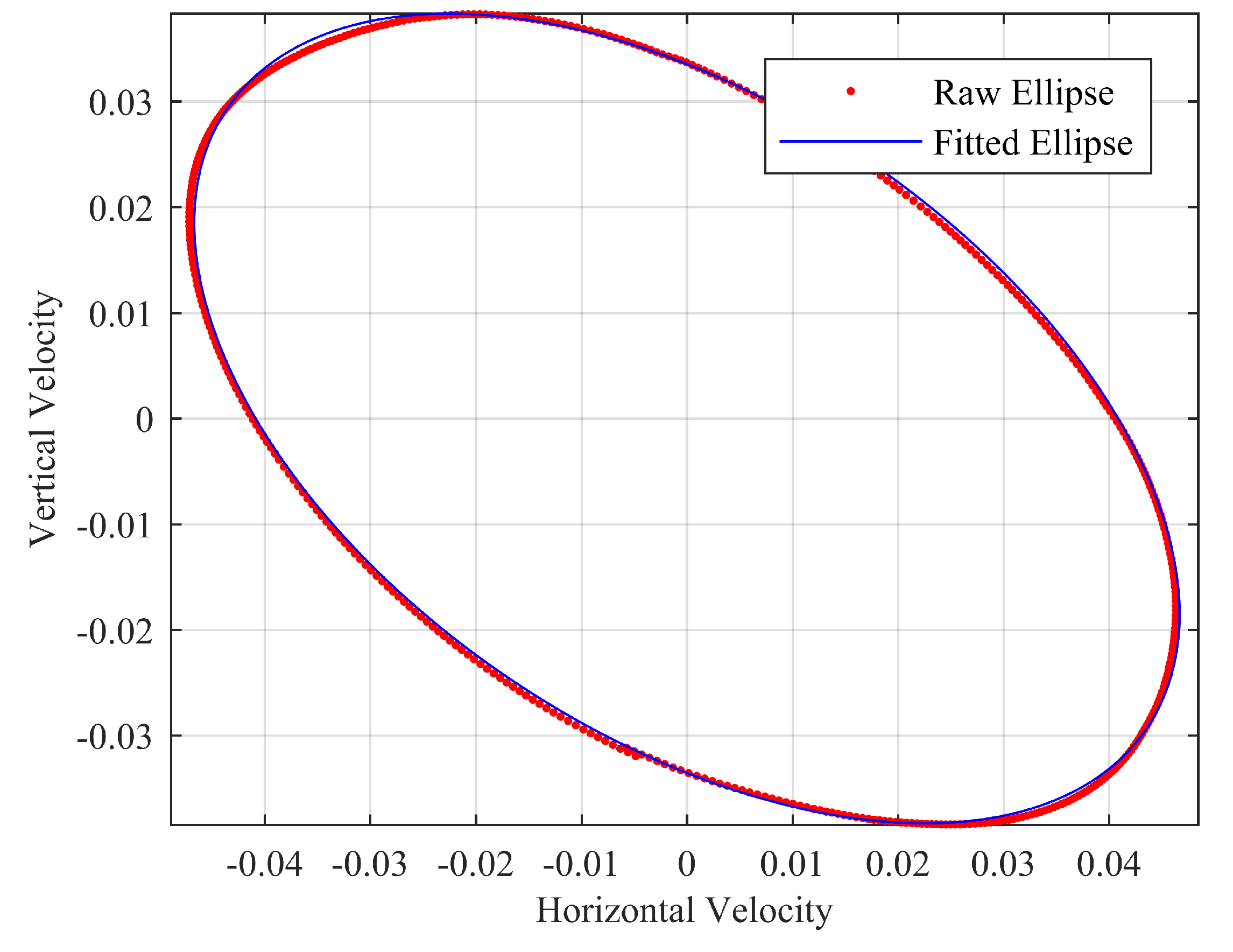
A data sample from the simulations is shown in Figure 5. The fitted ellipse had a maxima, minima and tilt of , and respectively. Additional wave parameters required for this calculation were obtained using a time trace of the velocity data over a single wave cycle (i.e., T = , = and z = ). The water depth was 1 m. The reflection coefficient can be seen in Table 5 (test case A).
5. Results
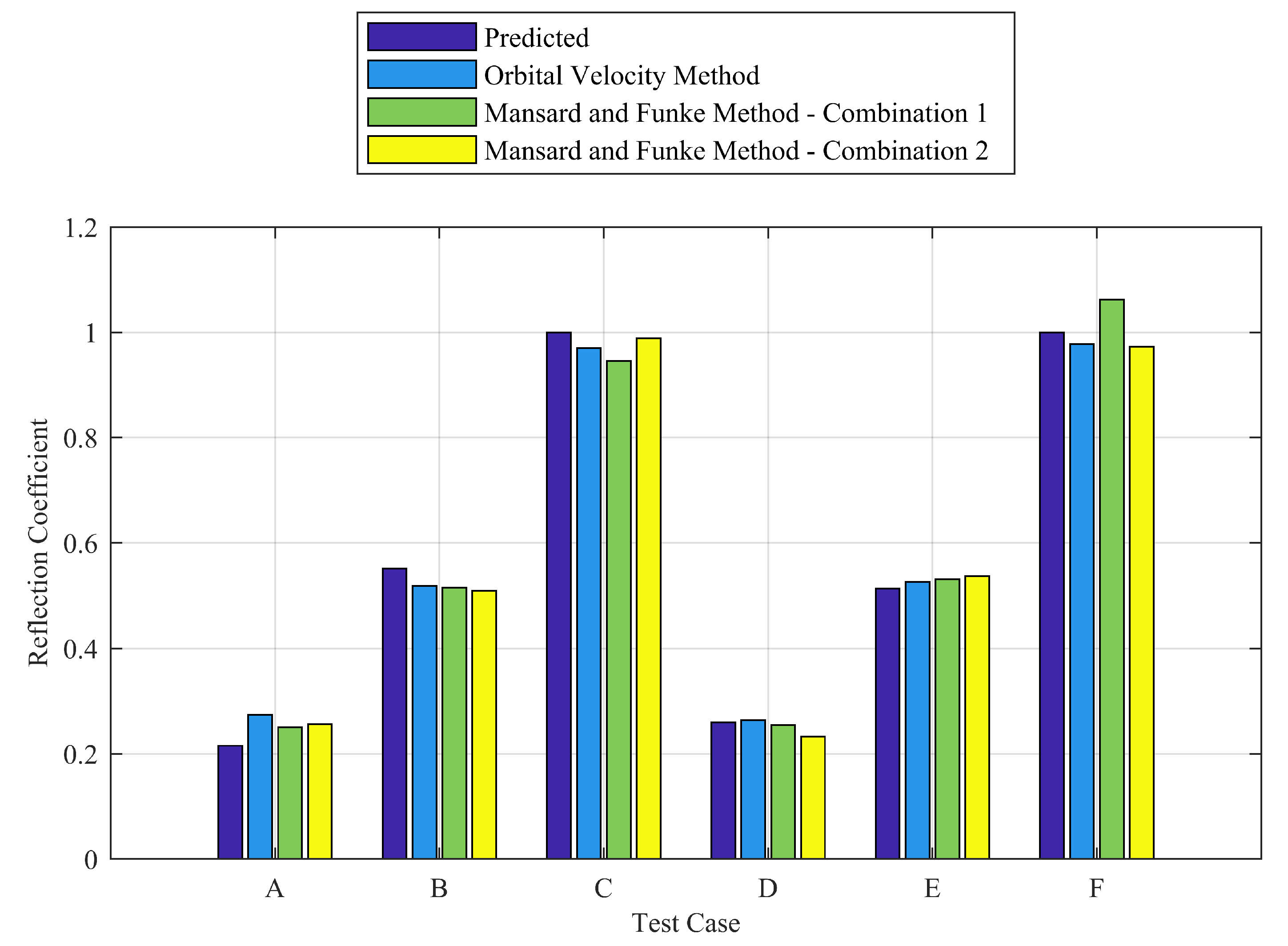
For each simulation, four reflection coefficients were calculated: one predicted based on the individual wavemaker data from the validation procedure as shown in Table 4, one using the Orbital Velocity method with the data from the best fitted ellipse and two from the Mansard and Funke method using two different surface elevation probe combinations described in Section 4. The results can be seen in Figure 6 and Table 5 and Table 6. Figure 6 presents the reflection coefficients obtained for all test cases investigated. The details of the test cases are described in Table 5 and Table 6.
Overall there is good agreement between all four reflection coefficients for each test case. With the exception of test case A, the Orbital Velocity method is consistently closer to the predicted reflection coefficient than at least one of the Mansard and Funke values with the majority of test cases being within 3%.
Test case F shows the largest deviation between the two reflection coefficients from the Mansard and Funke method. For all test cases the deviations between the Mansard and Funke values were less than 8.5%.
For test cases B, D, E and F there is good agreement between the Orbital Velocity method and at least one of the Mansard and Funke values. The agreement is less than 3% for the majority of test cases.
In addition, three velocity probes at the same location within the tank but at different depths below the water surface were included. The results in Table 5 and Table 6 are those which were calculated using velocities from the probe which was closest to the surface (Probe 1 in Table 1 and Table 2 for deep and intermediate water respectively). Table 7 summarises the calculated reflections at each probe depth in the deep water simulations. For the majority of test cases the deviation is less than 1%. The strongest agreement was in test case C.
6. Discussion
Differences between the reflection values dictated the use of the Mansard and Funke method and the Orbital Velocity method within the levels of experimental accuracy. Results obtained using the Orbital Velocity method were closer to the predicted reflection for the majority of test cases. The reason for the differences in the reflections obtained from Combinations 1 and 2 using the Mansard and Funke method is unclear and there is no known method to determine which value is the most accurate. This issue highlights the requirement for the Orbital Velocity method as it is able to quantify reflections using measurements from a single point.
The ideal position of the velocity probe for the Orbital Velocity method is expected to be close to the surface were velocities are larger. In the deep water simulations, the method was successful in obtaining accurate reflection coefficients to a depth of 40% of the water column. In deep water, the horizontal and vertical velocities decrease exponentially to zero below a depth of approximately half a wavelength. Beyond that, there is no wave induced velocity and thus measurements should not be taken in this region.
For intermediate and shallow water, the limitations are more difficult to predict accurately. According to analytical theory, in intermediate water the horizontal and vertical velocities decrease at different rates with depth and in shallow water only the vertical velocity decreases while the horizontal velocity remains constant. For both conditions the ellipse will be flat close to the tank bed as the vertical velocity is insignificant and thus the Orbital Velocity method is not applicable. It is unclear at this stage where in the water column the method begins to fail. This will depend on water depth, wavelength and height but further work is required to define the limiting conditions. In the simulations presented, the method could not yield reflection coefficients from the two lower probes in intermediate water, which measured in the lower 50% of the water column.
7. Conclusions and Future Work
This paper has presented a novel method to quantify reflections using the orbital velocities of water particles over a single wave cycle. Measurements are only required at one discrete location. It was demonstrated that reflection coefficients calculated using the novel Orbital Velocity method are at least as accurate as the Mansard and Funke method. Reflection coefficients obtained using the Orbital Velocity method also show better agreement with the predicted values. The Orbital Velocity method is thus a useful alternative to quantify reflection coefficients. The ability to use measurements from a single point renders the method particularly suitable in cases in which the waves are experiencing 3D effects such as directional spreading (e.g., an incident wave reflecting off a curved surface). Since it only requires a single wave cycle it is efficient, especially in computational modelling where long simulations, required for frequency domain analysis, are costly or may not even be feasible.
The only drawback to the method in its current form is the limitation to monochromatic seas. We predict that whilst this method could be extended to irregular waves in the future it would require a much larger data set than one wave cycle. However, as many investigations into reflection are performed in controlled environments (either numerical or physical) using monochromatic waves, the advantages such as being applicable to very short time traces, requiring just orbital velocity measurements at a single position (making experimental setup simpler) and being usable in cases affected by directional spreading, make it a valuable tool for the coastal and marine engineering industry.
Future work focuses on the application of the method to data from Acoustic Doppler Velocimeter (ADV) probes in physical tank tests. This will involve an investigation into the practical limitations of the method, including the vertical position of the velocity probe and the quality of the fitted ellipse.
References
Author Contributions
Conceptualization, B.E.; Data curation, P.S.; Formal analysis, R.M.; Methodology, R.M.; Software, P.S.; Supervision, B.E.; Writing—original draft, R.M. and P.S.; Writing—review and editing, R.M., B.E. and P.S.
Funding
This research received no external funding.
Acknowledgments
The authors wish to acknowledge the following funding bodies, which enabled them to undertake this work. The work undertaken by Rachael McKee has been supported by Engineering and Physical Sciences Research Council EPSRC (PID: M116317E). Björn Elsäßer has been supported by the European Community’s Horizon 2020 Programme through the grant to the budget of the Integrated Infrastructure Initiative HYDRALAB+ (Contract No.: 654110).
Conflicts of Interest
The authors declare no conflict of interest.
References
- O’Boyle, L.; Elsäßer, B.; Whittaker, T. Methods to enhance the performance of a 3D coastal wave basin. Ocean Eng. 2017, 135, 158–169. [Google Scholar] [CrossRef]
- Windt, C.; Davidson, J.; Schmitt, P.; Ringwood, J. Assessment of numerical wave makers. In Proceedings of the 12th European Wave and Tidal Energy Conference, Cork, Ireland, 27 August–1 September 2017. [Google Scholar]
- Thornton, E.B.; Calhoun, R.J. Spectral resolution of breakwater reflected waves. J. Waterw. Harbors Coast. Eng. Div. 1972, 98, 443–460. [Google Scholar]
- Goda, Y.; Suzuki, Y. Estimation of incident and reflected waves in random wave experiments. In Proceedings of the 15th Coastal Engineering Conference, Honolulu, Hawaii, 1–17 July 1976; pp. 828–845. [Google Scholar]
- Mansard, E.P.D.; Funke, E.R. The measurement of incident and reflected spectra using a least squares method. In Proceedings of the 17th Coastal Engineering Conference, Sydney, Australia, 23–28 March 1980; pp. 154–172. [Google Scholar]
- Lin, C.Y.; Huang, C.J. Decomposition of incident and reflected higher harmonic waves using four wave gauges. Coast. Eng. 2004, 51, 395–406. [Google Scholar] [CrossRef]
- Viviano, A.; Naty, S.; Foti, E.; Bruce, T.; Allsop, W.; Vicinanza, D. Large-scale experiments on the behaviour of a generalised Oscillating Water Column under random waves. Renew. Energy 2016, 99, 875–887. [Google Scholar] [CrossRef] [Green Version]
- Isaacson, M. Measurement of regular wave reflection. J. Waterw. Port Coast. Ocean Eng. 1991, 117, 553–569. [Google Scholar] [CrossRef]
- Frigaard, P.; Brorsen, M. A time-domain method for separating incident and reflected irregular waves. Coast. Eng. 1995, 24, 205–215. [Google Scholar] [CrossRef] [Green Version]
- Ursell, F.; Dean, R.G.; Yu, Y.S. Forced small-amplitude water waves: A comparison of theory and experiment. J. Fluid Mech. 1960, 7, 33–52. [Google Scholar] [CrossRef]
- Madsen, P.A. Wave reflection from a vertical permeable wave absorber. Coast. Eng. 1983, 7, 381–396. [Google Scholar] [CrossRef]
- Baldock, T.; Simmonds, D. Separation of incident and reflected waves over sloping bathymetry. Coast. Eng. 1999, 38, 167–176. [Google Scholar] [CrossRef]
- Brossard, J.; Hémonb, A.; Rivoalena, E. Improved analysis of regular gravity waves and coefficient of reflexion using one or two moving probes. Coast. Eng. 2000, 39, 193–212. [Google Scholar] [CrossRef]
- Hughes, S.A. Laboratory wave reflection analysis using co-located gages. Coast. Eng. 1993, 20, 223–247. [Google Scholar] [CrossRef]
- Hughes, S.A. Physical Models and Laboratory Techniques in Coastal Engineering; Advanced Series on Ocean Engineering; World Scientific: Singapore, 1993; Chapter 4; Volume 7. [Google Scholar]
- Neves, C.F.; Endres, L.A.M.; Fortes, C.J.; Clemente, D.S. The use of ADV in wave flumes: Getting more information about waves. Coast. Eng. Proc. 2012, 1, 38. [Google Scholar] [CrossRef]
- Brede, H. Reflection Analysis of a new Gravel Beach Arrangement in Portaferry Wave Basin; Technical Report; Queen’s University Belfast: Belfast, UK, 2013. [Google Scholar]
- Lamont-Kane, P.; Folley, M.; Whittaker, T. Investigating uncertainties in physical testing of wave energy converter arrays. In Proceedings of the 10th European Wave and Tidal Energy Conference (EWTEC 2013), Aalborg, Denmark, 2–5 September 2013. [Google Scholar]
- Peric, R.; Abdel-Maksoud, M. Assessment of uncertainty due to wave reflections in experiments via numerical flow simulations. In Proceedings of the International Offshore and Polar Engineering Conference, Kona, HI, USA, 21–26 June 2015; pp. 530–537. [Google Scholar]
- Schmitt, P.; Elsaesser, B. A review of wave makers for 3D numerical simulations. In Proceedings of the Marine 2015 6th International Conference on Computational Methods in Marine Engineering, Rome, Italy, 15–17 June 2015; pp. 437–446. [Google Scholar]
- Schmitt, P.; Doherty, K.; Clabby, D.; Whittaker, T. The opportunities and limitations of using CFD in the development of wave energy converters. In Proceedings of the RINA Marine and Offshore Energy Conference, London, UK, 26–27 September 2012; pp. 89–97. [Google Scholar]
- Tezdogan, T.; Incecik, A.; Turan, O. Full-scale unsteady {RANS} simulations of vertical ship motions in shallow water. Ocean Eng. 2016, 123, 131–145. [Google Scholar] [CrossRef]
- Vanneste, D.; Troch, P. 2D numerical simulation of large-scale physical model tests of wave interaction with a rubble-mound breakwater. Coast. Eng. 2015, 103, 22–41. [Google Scholar] [CrossRef]
- Schmitt, P.; Elsäßer, B. On the use of OpenFOAM to model oscillating wave surge converters. Ocean Eng. 2015, 108, 98–104. [Google Scholar] [CrossRef] [Green Version]
- Devolder, B.; Stratigaki, V.; Troch, P.; Rauwoens, P. CFD Simulations of Floating Point Absorber Wave Energy Converter Arrays Subjected to Regular Waves. Energies 2018, 11, 641. [Google Scholar] [CrossRef]
- Olbert, G.; Schmitt, P. Steps towards fully nonlinear simulations of arrays of OWSC. In Proceedings of the 19th Numerical Towing Tank Symposium, St. Pierre d’Oleron, France, 3–4 October 2016. [Google Scholar]
- McKee, R.; Elsaesser, B.; O’Boyle, L. Investigating Tools used to Analyse the Impact of a Wave Farm on the surrounding Wave Field. In Proceedings of the 12th European Wave and Tidal Energy Conference, Cork, Ireland, 27 August–1 September 2017. [Google Scholar]
- O’Boyle, L.; Elsäßer, B.; Whittaker, T. Experimental Measurement of Wave Field Variations around Wave Energy Converter Arrays. Sustainability 2017, 9, 70. [Google Scholar] [CrossRef]
- Dean, R.G.; Dalrymple, R.A. Water Wave Mechanics for Engineers and Scientists; Advanced Series on Ocean Engineering; World Scientific: Singapore, 1984; Chapter 4; Volume 2, pp. 78–130. [Google Scholar]
- Wallet, A.; Ruellan, F. Free-surface flow. In An Album of Fluid Motion; The Parabolic Press: Stanford, CA, USA, 1982; Chapter 7; pp. 110–111. [Google Scholar]
- Peric, R.; Abdel-Maksoud, M. Analytical prediction of reflection coefficients for wave absorbing layers in flow simulations of regular free-surface waves. Ocean Eng. 2018, 147, 132–147. [Google Scholar] [CrossRef] [Green Version]
Figure 1.
Schematic representation of water particle velocities where h is the water depth and is the wavelength for different water depths.
Figure 1.
Schematic representation of water particle velocities where h is the water depth and is the wavelength for different water depths.
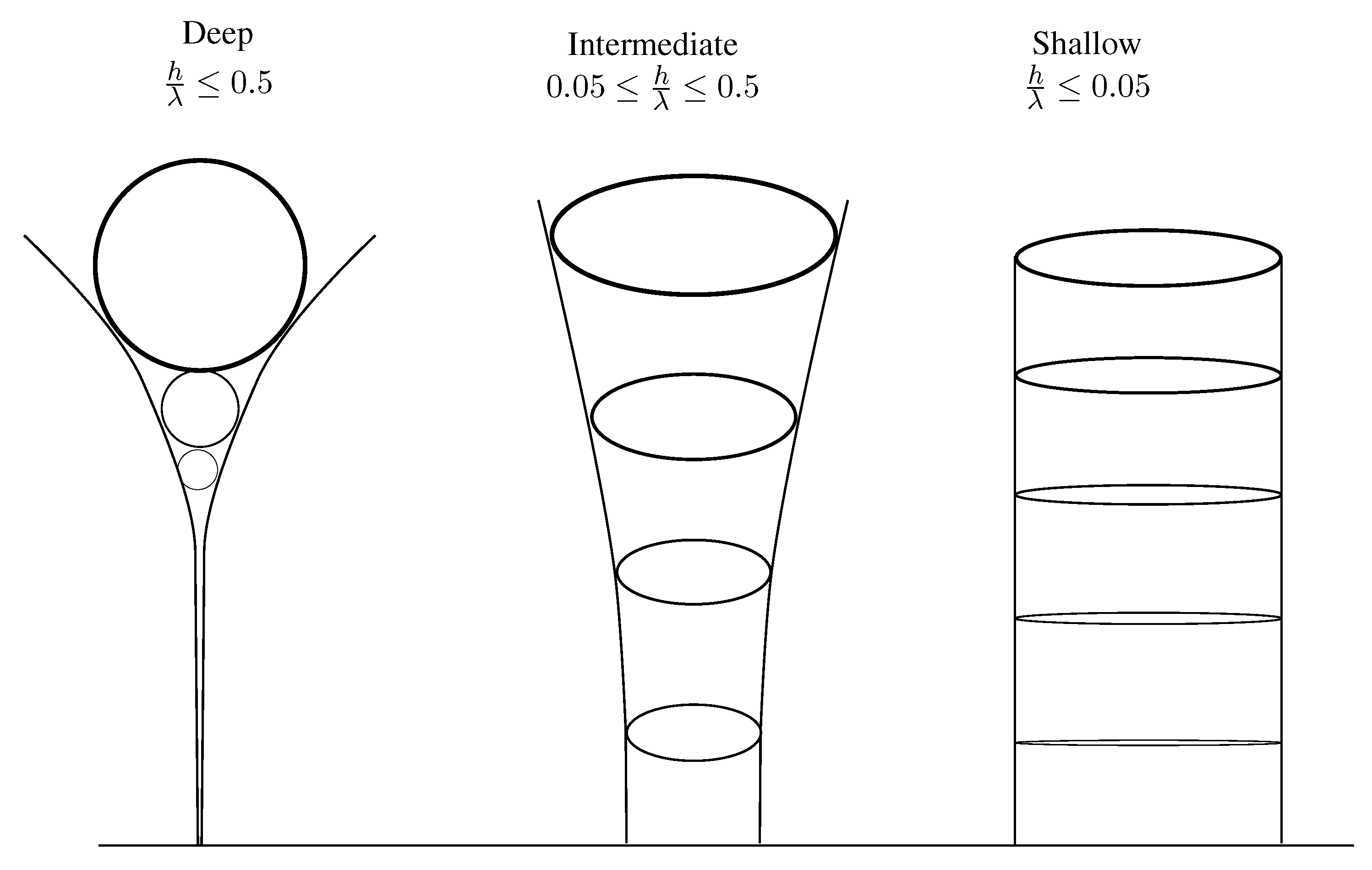
Figure 2.
Schematic representation of the cross section of an incident and reflected wave in deep water where and are the horizontal and vertical velocity components for the incident wave, and are the horizontal and vertical velocity components for the reflected wave, and are the horizontal and vertical velocity components for the resultant wave, d is the distance of x to the reflective boundary, x is the horizontal distance, z is the vertical depth from the still water surface and is the tilt of the maxima axis to the horizontal axis.
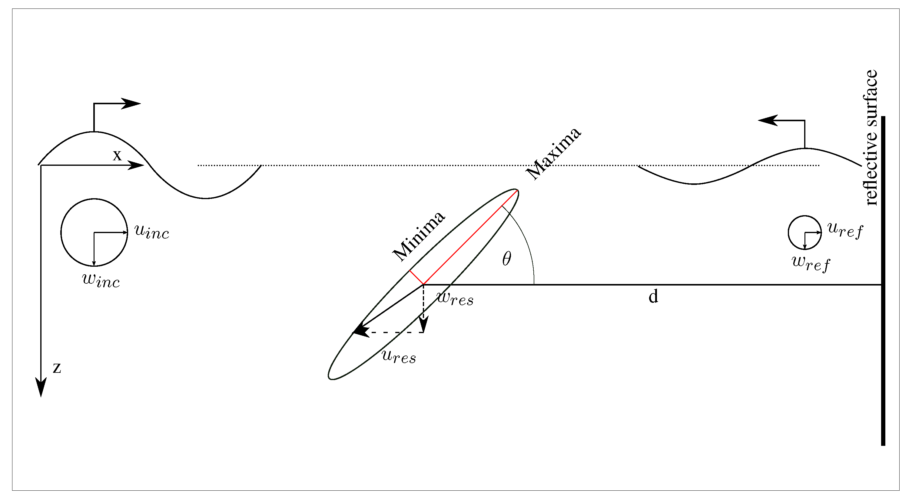
Figure 3.
Flow chart of the Orbital Velocity method where is the reflection coefficient, is the tilt of the ellipse of the dataset and .
Figure 3.
Flow chart of the Orbital Velocity method where is the reflection coefficient, is the tilt of the ellipse of the dataset and .
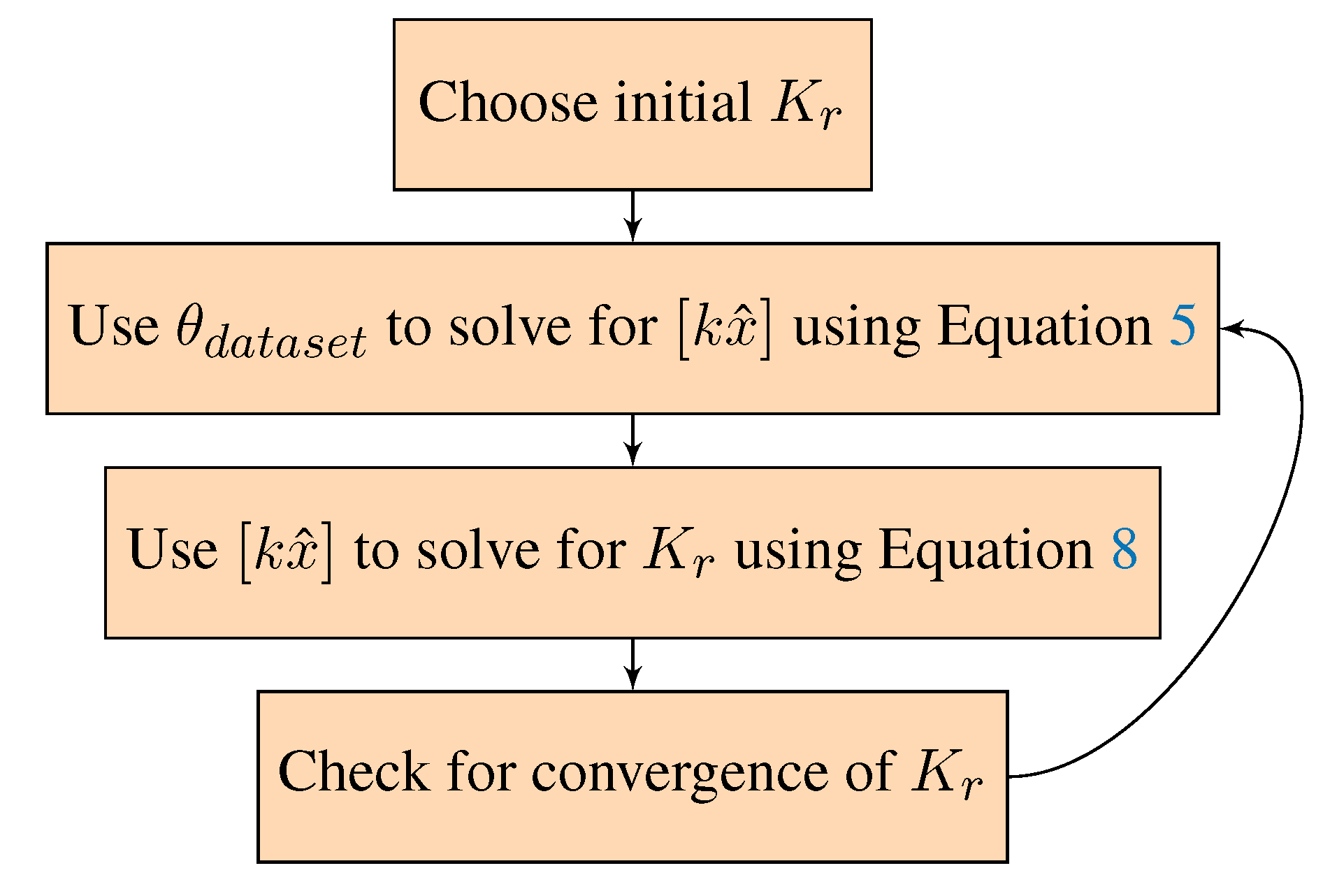
Figure 4.
Definition of numerical beaches and wave maker regions.
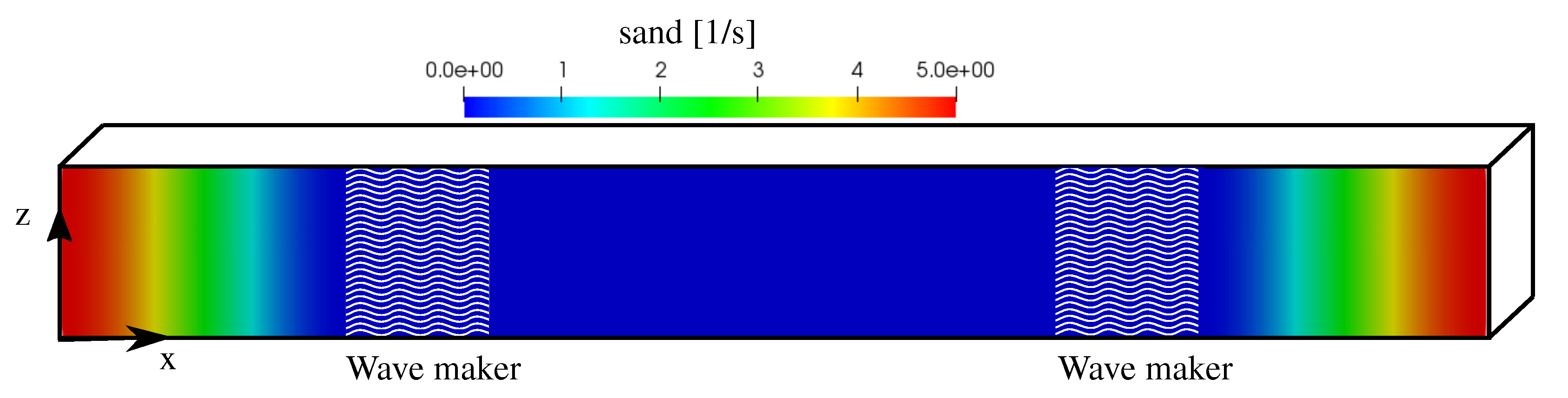
Figure 5.
Orbital velocity trace fitted with an ellipse.


Table 1.
Velocity probe positions for deep water simulations.
| Probe | X (m) | Y (m) | Z (m) |
|---|---|---|---|
| 1 | 5.0 | 0.05 | 0.8 |
| 2 | 5.0 | 0.05 | 0.7 |
| 3 | 5.0 | 0.05 | 0.6 |
Table 2.
Velocity probe positions for intermediate water simulations.
| Probe | X (m) | Y (m) | Z (m) |
|---|---|---|---|
| 1 | 5.0 | 0.05 | 0.2 |
| 2 | 5.0 | 0.05 | 0.15 |
| 3 | 5.0 | 0.05 | 0.1 |
Table 3.
Surface elevation gauge positions.
| Probe | X (m) |
|---|---|
| 1 | 4.5 |
| 2 | 4.7 |
| 3 | 5.0 |
| 4 | 5.5 |
| 5 | 6.7 |
Table 4.
Wave height associated with each wave maker.
| Wave Maker Number | Water Depth (m) | Wave Height (m) |
|---|---|---|
| 1 | 0.0059 | |
| 2 | 1.0 | 0.0151 |
| 3 | 0.0274 | |
| 4 | 0.0090 | |
| 5 | 0.3 | 0.0179 |
| 6 | 0.0349 |
Table 5.
Reflection coefficients using different methods from the deep water ( ) simulations.
| Reflection Coefficient | |||||
|---|---|---|---|---|---|
| Test Case | Wave Makers | Predicted | Orbital Velocity | Mansard and Funke Method | |
| Method | Combination 1 | Combination 2 | |||
| A | 1 and 3 | 0.22 | 0.27 | 0.25 | 0.26 |
| B | 2 and 3 | 0.55 | 0.52 | 0.52 | 0.51 |
| C | 3 and 3 | 1.00 | 0.97 | 0.95 | 0.99 |
Table 6.
Reflection coefficients using different methods from the intermediate water ( ) simulations.
Table 6.
Reflection coefficients using different methods from the intermediate water ( ) simulations.
| Reflection Coefficient | |||||
|---|---|---|---|---|---|
| Test Case | Wave Makers | Predicted | Orbital Velocity | Mansard and Funke Method | |
| Method | Combination 1 | Combination 2 | |||
| D | 4 and 6 | 0.26 | 0.26 | 0.25 | 0.23 |
| E | 5 and 6 | 0.51 | 0.53 | 0.53 | 0.54 |
| F | 6 and 6 | 1.00 | 0.98 | 1.06 | 0.97 |
Table 7.
Reflection coefficients for probes of varying vertical positions in deep water ( 1 ) simulations.
Table 7.
Reflection coefficients for probes of varying vertical positions in deep water ( 1 ) simulations.
| Test Case | ||||||
|---|---|---|---|---|---|---|
| Distance from Seabed (m) | A | B | C | |||
| Error | Error | Error | ||||
| 0.8 | 0.27 | 0.52 | 0.97 | |||
| 0.7 | 0.28 | 3.1% | 0.54 | 3.8% | 0.96 | −1% |
| 0.6 | 0.27 | 0% | 0.52 | 0% | 0.98 | 1% |
© 2018 by the authors. Licensee MDPI, Basel, Switzerland. This article is an open access article distributed under the terms and conditions of the Creative Commons Attribution (CC BY) license (http://creativecommons.org/licenses/by/4.0/).
Share and Cite
MDPI and ACS Style
McKee, R.; Elsäßer, B.; Schmitt, P. Obtaining Reflection Coefficients from a Single Point Velocity Measurement. J. Mar. Sci. Eng. 2018, 6, 72. https://doi.org/10.3390/jmse6020072
AMA Style
McKee R, Elsäßer B, Schmitt P. Obtaining Reflection Coefficients from a Single Point Velocity Measurement. Journal of Marine Science and Engineering. 2018; 6(2):72. https://doi.org/10.3390/jmse6020072
Chicago/Turabian StyleMcKee, Rachael, Björn Elsäßer, and Pál Schmitt. 2018. "Obtaining Reflection Coefficients from a Single Point Velocity Measurement" Journal of Marine Science and Engineering 6, no. 2: 72. https://doi.org/10.3390/jmse6020072
Note that from the first issue of 2016, this journal uses article numbers instead of page numbers. See further details here.