Nominal vs. Effective Wake Fields and Their Influence on Propeller Cavitation Performance


1
Department of Mechanical Engineering, Technical University of Denmark, Nils Koppels Allé 403, 2800 Kgs. Lyngby, Denmark
2
MAN Diesel & Turbo, Engineering and R&D Propulsion, 2450 København SV, Denmark
*
Author to whom correspondence should be addressed.
J. Mar. Sci. Eng. 2018, 6(2), 34; https://doi.org/10.3390/jmse6020034
Submission received: 27 February 2018
/
Revised: 25 March 2018
/
Accepted: 29 March 2018
/
Published: 5 April 2018
(This article belongs to the Special Issue Marine Propulsors)
Abstract
:Propeller designers often need to base their design on the nominal model scale wake distribution because the effective full scale distribution is not available. The effects of such incomplete design data on cavitation performance are examined in this paper. The behind-ship cavitation performance of two propellers is evaluated, where the cases considered include propellers operating in the nominal model and full scale wake distributions and in the effective wake distribution, also in the model and full scale. The method for the analyses is a combination of RANS for the ship hull and a panel method for the propeller flow, with a coupling of the two for the interaction of ship and propeller flows. The effect on sheet cavitation due to the different wake distributions is examined for a typical full-form ship. Results show considerable differences in cavitation extent, volume, and hull pressure pulses.
1. Introduction
1.1. Motivation
Propeller cavitation is strongly influenced by the non-uniform inflow to the propeller. As the ship wake is dominated by viscous effects, it is subject to major scale effects. Still, propeller designers are generally only provided with the nominal wake field measured at model scale. This then needs to be scaled to match the estimated full scale effective wake fraction from a self-propulsion test to ensure that the average axial velocity in the propeller disk corresponds to the average effective inflow. However, scaling the field uniformly will not result in the right velocity distribution. In addition to the scale effects, the actual inflow field to the propeller is not the nominal field, but the effective wake field, including hull–propeller interaction. As a result, the propeller designer might base design decisions on insufficiently accurate information.
A successful propeller design is a trade-off between propeller cavitation performance and total propeller efficiency. The ability to predict cavitation performance at early design stages will eliminate the need for overly conservative designs. This paper intends to highlight the role of the wake field in the design, analysis, and optimization of a conventional ship propeller.
1.2. Background
Due to the higher Reynolds number at full scale compared to model scale, the boundary layer around the ship hull changes and hence the velocity distribution near the hull is altered. This difference results in a narrower wake peak and a lower wake fraction in full scale. The presence of the propeller behind the ship adds to the complexity of the problem because the propeller–hull interaction modifies the inflow field to the propeller as well.
Single-screw ship wake fields are usually characterized by a strongly non-uniform distribution of velocities with a wake peak at the 12 o’clock position, where the axial velocities are particularly low. This means that the blade sections of a propeller operating behind the ship experience strong variations in angle of attack. As the hydrostatic pressure acting on the blade reaches its minimum at the same time as the blade experiences high angles of attack while passing through the wake peak, this region of the wake field is particularly critical in terms of cavitation.
Analyzing the different factors influencing propeller cavitation and related erosion and vibration issues, an ITTC propulsion committee [1] pointed out that, for large container ships with highly-loaded propellers, the wake field characteristics—and not propeller geometry details—are the key to achieving decent propeller cavitation performance.
Especially the depth of the wake peak, i.e., the difference between the lowest axial velocity occurring there and the maximum velocity in the propeller disk, is of decisive importance for the cavitation performance of a propeller behind the ship. When uniformly scaling the nominal wake velocities to match the effective wake fraction, the width and depth of the wake peak are unlikely to be represented properly.
As this has been known for many years, different methods exist for estimating the full scale wake field of a ship, covering a rather wide range of complexity and sophistication. Usually the nominal wake field, measured at model scale, serves as input for these methods. A review of the most commonly used scaling methods was carried out some years ago by an ITTC specialist committee on wake field scaling [2]. That report mentions the simplest form of wake scaling, where one only scales the wake field by changing the magnitude of the velocities uniformly to match a target wake fraction, as already described above. In that case, the shape of the isolines of the input field (usually the measured nominal wake field) remains unchanged. Therefore, even calling this procedure a “scaling method” is questionable. While the shortcomings of this approach are well-known, it still appears to be commonly used for its simplicity.
Adding complexity while still only requiring very limited effort, the semi-empirical scaling method described by Sasajima and Tanaka [3] decomposes the wake into a frictional and potential component and contracts the frictional wake based on horizontal velocity profiles. This still-popular method was recommended (with warnings) by the above-mentioned ITTC committee in 2011 for the case when full scale wake data are not available.
The main challenges related to scale effects on the effective wake field and the corresponding effect on propeller cavitation are outlined in a review by van Terwisga et al. [4]. The work by Bosschers et al. [5] is one of the relatively few examples that explicitly show and discuss differences in propeller cavitation due to the effect of hull–propeller interaction and local changes in the wake distribution. That paper focuses on scale effects, offers comparisons with experiments at model and full scale, and uses similar methods as the present work for computation of effective wake fields and sheet cavitation prediction.
Gaggero et al. [6] compared the cavitation performance of conventional propellers in nominal full scale wake fields from CFD calculations to the performance in nominal full scale wake fields obtained by applying an empirical wake scaling method to measured nominal fields at model scale, and observed noticeable differences.
The present work focuses on the differences in predicted sheet cavitation behavior purely due to the wake distribution, using computed nominal and effective wake fields at both model and full scale. Section 4 presents analysis results for one propeller and different wake distributions. Section 5 introduces another propeller designed for the same ship, showing the difference in cavitation behavior between propellers designed for different wake distributions.
2. Methods
2.1. Boundary Element Method for Propeller Analysis
A potential-based boundary element method (“panel code”) serves as the main tool for propeller analysis in the present work. As for all potential flow-based methods, inviscid, incompressible, and irrotational flow is assumed. Sheet cavitation is modeled in a partially nonlinear way. The present implementation’s approach to cavitation modeling—whose basic formulation is reproduced below—follows the approach initially introduced by Kinnas and Fine [7] and is able to predict unsteady sheet cavitation in inhomogeneous inflow, including supercavitation.
Mathematical Formulation
The velocity potential must satisfy the Laplace equation:
Given the linearity of Equation (1), the total velocity vector can be split into a known onset part (dependent on the wake field with the local velocity and the propeller rotation) and the gradient of a propeller geometry-dependent perturbation potential that is to be determined:
For a domain bound by the blade surface (with a continuous distribution of sources and dipoles) and the force-free wake surface (with a continuous distribution of dipoles), application of Green’s second identity gives the potential at a field point p, when the integration point q lies on the domain boundary. G is defined as the inverse of the distance R between these two points, . The term corresponds to the potential jump across the wake sheet at an integration point q on . An additional term appears in the presence of supercavitation, as additional sources—with the strength —are placed on the cavitating part of the wake, .
If the field point p lies on the blade surface, the potential is found from
As the surface in principle consists of two surfaces collapsed into one infinitely thin wake sheet, the integral equation reads slightly differently if the field point lies on . The potential for a field point on the wake surface is
Equations (3) and (4) are then discretized using flat quadrilateral panels arranged in a structured mesh. Introducing influence coefficient matrices through that describe the influence from unit strength singularities located on panel j on the control point of panel i, a system of equations and unknowns results. For each panel on the blade, one equation of the following form exists:
and, for each cavitating wake panel, there is an additional equation of the form
On the wetted part of the blade, the source strengths are known from the kinematic boundary condition, Equation (8), and the dipole strength is the unknown:
On the cavitating part of the blade and wake surfaces, a dynamic boundary condition is applied, prescribing the pressure to correspond to the given cavitation number . To achieve this, the corresponding local “cavity velocity” needs to be found. For convenience, this part is formulated in curvilinear coordinates aligned with the panel edges. The v-direction is pointing outwards in the spanwise direction and the s-direction is the chordwise direction, positive towards the trailing edge on the suction side of the blade. The angle between the and vectors of a panel is designated and is usually close to 90. With and as the s- and v-components of the onset velocity vector and z as the vertical distance from the propeller shaft, the chordwise cavity velocity corresponding to the cavitation number at shaft depth is
where
To be able to provide a Dirichlet boundary condition on the potential, Equation (9) is integrated in chordwise direction and added to the potential at the chordwise detachment point , which is assumed known and practically expressed by extrapolation from the wetted part ahead of the cavity:
The cavity extent on the blade (and wake) needs to be found iteratively. After an initial guess based on the non-cavitating pressure distribution and cavitation number, the cavity thickness is computed. The cavity extent is then changed until the cavity thickness is sufficiently close to zero at the edges of the cavity sheet, so it detaches from the blade and closes on the blade or wake. For the cavity closure, the pressure recovery model described in [7] is used.
The present implementation also includes additional features described in [8], such as the split panel technique for faster convergence and more flexibility in terms of mesh and timestep size. However, the present implementation (the panel code “ESPPRO”, developed at the Technical University of Denmark), uses lower-order extrapolation schemes throughout for increased numerical stability. In addition, spatial derivatives in the cavity height equation are discretized using lower-order finite differences.
2.2. RANS-BEM Coupling
In recent years, viscous flow simulations around the hull coupled with potential flow-based propeller models have become a popular choice for numerical self-propulsion simulations. Usually, field methods solving the Reynolds-averaged Navier–Stokes (RANS) equations are used for the hull part, and panel methods (boundary element methods, BEM) are a common choice for the propeller calculations, as they allow for a good representation of the flow physics while only requiring limited computational effort. Computational approaches using this combination of tools are commonly called “RANS-BEM Coupling”.
In such an approach, the exact propeller geometry is not resolved in CFD, but the propeller is accounted for by modeling its effect on the flow by introducing body forces, provided by the propeller model. This is an iterative process: the total velocity field in the coupling plane (an approximation of the propeller plane) is passed from the RANS solver to the propeller model, which then returns the propeller forces that correspond to this inflow field. The key part here is that the inflow field to the propeller model is not the total wake field as extracted from the global CFD simulation, but rather the effective wake field, i.e., with the propeller-induced velocities subtracted from the total wake field. The induced velocity field is approximated by using the values from the previous coupling iteration. Thereby, the effective wake field is not only a byproduct but also an inherent part of this iterative coupling.
By being able to compute not only the effective wake fraction but also the distribution of the effective wake velocities in the propeller disk, the RANS-BEM coupling approach provides a major advantage over all CFD simulations beyond substantially reducing the computational effort.
In the present work, the RANS-BEM coupling approach is used to determine effective wake fields at model and full scale to later investigate differences in propeller cavitation. On the RANS side, the XCHAP solver from the commercial Shipflow package is used. XCHAP solves the steady-state RANS equations on overlapping, structured grids using the finite volume method and employs the EASM (Explicit Algebraic Stress Model) turbulence model. Nominal wake fields are found using the same RANS solver and identical grids, but with the propeller model switched off.
The DTU-developed panel code ESPPRO (whose basic formulation is described in the previous section) serves as the propeller model. The unsteady propeller forces are time-averaged over one revolution before being passed to XCHAP. In line with that, the induced velocity field is also time-averaged to compute the effective wake field in the subsequent coupling iteration.
When modeling the propeller in RANS by a body force distribution only, the blade blockage effect is present in the BEM, but not transferred to the RANS side of the computation. The implications of this are shown in [11], which also discusses two possibilities to address this problem in a consistent manner: either by accounting for the blockage on the RANS side by mass sources, or by removing the blockage from the BEM side. In the present work, the latter option—the approach initially described in [12]—is followed, excluding the contribution of all sources when computing forces and velocities used as part of the RANS-BEM coupling.
To reduce computational effort, the non-cavitating condition is assumed in self-propulsion and the cavitation model described previously remains disabled. This is not expected to have a noticeable effect on the computed effective wake distributions, as in the present model a sheet cavity is primarily represented by the presence of additional sources. As mentioned above, sources do not contribute to relevant quantities used in the RANS-BEM coupling. The remaining relevant effect of the sheet cavity on the computed effective wake field, the change in the dipole strength distribution on the blade, is considered negligibly small for the expected cavitation extent.
Previous work on computing effective wake fields using RANS-BEM coupling by Rijpkema et al. [12] highlighted the importance and influence of the location of the coupling plane on self-propulsion results. As singularities are placed on the propeller blade surfaces in the panel method, the induced velocities can not be computed in the propeller plane directly. To avoid evaluating induced velocities too close to the singularities, the coupling plane is usually chosen to be upstream of the propeller. Extrapolating the effective wake to the propeller plane linearly from two upstream planes was found [12] to give the best results in terms of predicting the self-propulsion point (effective wake fraction in self-propulsion).
For the present work, the distribution of effective velocities in the coupling plane is of higher interest than the mean velocity, i.e., the absolute value of the wake fraction. Therefore, and to remove any potential extrapolation artifacts that affect the distribution, the effective wake is computed on a single curved surface that follows the blade leading edge contour closely (at an axial distance of 2% of the propeller diameter), essentially resulting in a curved coupling plane just upstream of the propeller.
3. Case Study
All calculations are carried out for a state-of-the-art handysize bulk carrier, representing a modern single-screw full hull form. The block coefficient is 0.82 and the aftbody is of pram-with-gondola-type. The simple conventional propeller used for the analyses was specifically designed for this ship and the present work (see Section 5 for more details on the design method).
In this work, nominal wake fields at model and full scale for this ship are obtained by running steady-state RANS-based CFD simulations. Effective wake fields at the self-propulsion point, also at both model and full scale, are computed using the hybrid RANS-BEM method described in the previous section. Additionally, Sasajima’s wake scaling method is applied to the computed model scale nominal wake field for comparison with the computed full scale fields.
The effect of the wake distribution on propeller cavitation performance, including cavitation extent, cavitation volume, and hull pressure pulses, is examined by using the panel code with the sheet cavitation model described in Section 2.1.
For the cavitation analyses, the axial components of all five wake fields (nominal and effective at model and full scale, plus the result of Sasajima’s scaling method) are then uniformly scaled to the same axial wake fraction, so the propeller is running at the same operating point in all wake fields. Any differences in results are then due to the different velocity distributions in the propeller disk and different in-plane velocity components.
All cavitation simulations are carried out at a cavitation number (based on the propeller speed n) of , corresponding to the full scale condition. The propeller for this ship is moderately loaded () at the operating point considered.
Note that approach, case, and all simulation conditions are identical to those used in the earlier version of the present work, presented and published by the authors at the Fifth International Symposium on Marine Propulsors (smp’17) [13]. Nominal and effective wake fields are unchanged, while there are differences in cavitation simulation results. These differences are due to changes made to the ESPPRO code and the corresponding preprocessor. The improvements allow for higher spatial resolution and higher-quality meshes, and an improved cavity shape-finding mechanism that reduces the openness tolerance by one order of magnitude compared to previous versions. Apart from increasing accuracy, the latter also affects the rate at which the cavity can grow and shrink. The present results thereby reflect progress made between January 2017 and January 2018. The authors are not aware of major problems in either of the two versions, and the results primarily differ in magnitude, showing the same trends and leading to the same conclusions.
4. Results and Discussion
4.1. Wake Fields
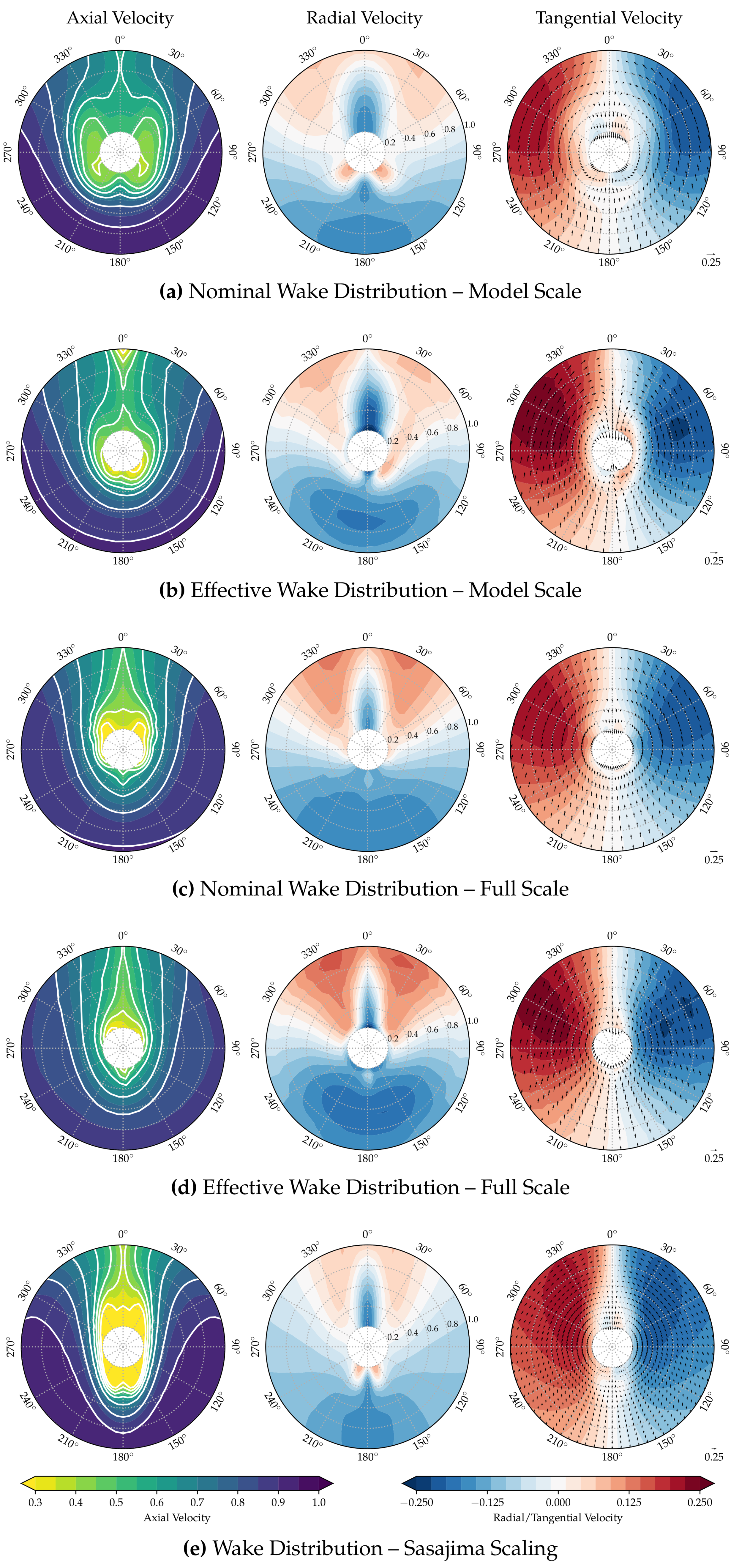
Figure 1a–d show the nominal and effective wake distributions based on the RANS and RANS-BEM results. Figure 1e shows the full scale wake field after applying Sasajima’s scaling method, based on the computed nominal wake at model scale and the potential wake (see Figure 2), computed using the panel code Shipflow-XPAN.
Note, however, that all fields shown have been “scaled” or “corrected” to match the same axial wake fraction of 0.25. This value corresponds to the full scale prognosis for the effective wake fraction based on model tests with a stock propeller for a ship very similar to the case considered here. Apart from this number, no further model test results have been used in any part of this work. For an original wake fraction and a target value of , the “corrected” non-dimensional axial velocity u at any point is , where is the original non-dimensional axial velocity at that point and .
The uncorrected wake fractions are listed in Table 1. As expected, the wake fractions of the model scale fields are substantially higher than the fractions in full scale, and the computed effective wake fractions are lower than their nominal counterparts. Applying Sasajima’s semi-empirical scaling method to the computed nominal model scale wake field results in a wake fraction that is surprisingly close to the computed effective wake fraction in full scale. Still, while the axial wake fractions are similar, the differences in axial and radial wake distribution are substantial, as can be seen from Figure 1d,e.
A strong bilge vortex can be seen in Figure 1a, which results in low axial velocities in the region between the hub and 40% of the propeller radius. It should be noted that, in this radial range of this particular wake field, the axial velocities in the usual “wake peak” region between 330 and 30 are actually higher than in the lower half of the field.
Looking at the effective wake distribution resulting from the self-propulsion simulation at model scale, Figure 1b, the bilge vortex appears substantially weaker and closer to the centerline. This is also obvious from the radial and tangential velocity components, which are otherwise of similar magnitude as in Figure 1a. The effective field shown in Figure 1b exhibits a much more defined and pronounced wake peak at 12 o’clock, the axial velocities reaching consistently low values in this region.
The asymmetric flow at the innermost radii seen in Figure 1b is attributed to the lack of the propeller hub in both the RANS and the BEM part of the simulation. No propeller shaft, hub, or even stern tube was part of the RANS grids. The lack of the hub in the propeller panel code results in an unrealistic flow around the open blade root. Consequently, secondary flow structures emerge at low Reynolds numbers. While undesirable, the effect is local and is not expected to influence the cavitation behavior. As can be seen in Figure 1d, this is of less concern at full scale.
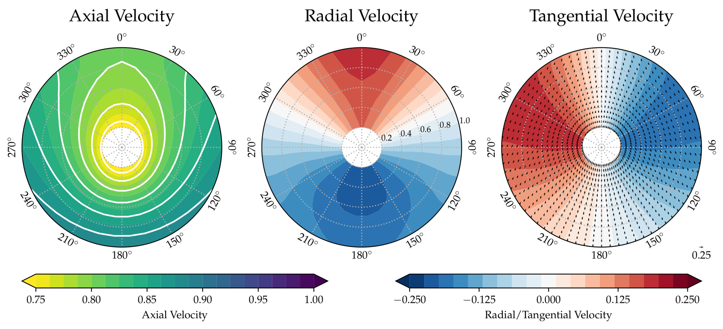
Moving to full scale, the nominal wake distribution (Figure 1c) changes significantly compared to model scale, as expected. The bilge vortex is remarkably less dominant, and the isolines of the axial wake distribution are more U-shaped. With a thinner boundary layer and a weaker bilge vortex, the in-plane velocity components change as well. In both computed full scale fields, the radial and tangential components indicate a less vortical and more upwards-directed flow. Except for the remainders of the bilge vortex, the in-plane velocity distribution approaches the potential one (Figure 2).
The trend towards a more defined and narrower wake peak continues moving on to the effective wake distribution at full scale, shown in Figure 1d. A bilge vortex can hardly be observed anymore.
Applying the method by Sasajima and Tanaka [3] leads to a very different wake distribution. The method works by contracting the nominal model scale wake field horizontally while also scaling the axial velocities, depending on the relationship of frictional and potential wake. For this particular case—with the above-described flow features in the nominal wake field at model scale—this results in a box-shaped region of very low axial velocities, visible in Figure 1e. Given that all fields shown in Figure 1 are uniformly scaled to the same wake fraction, the velocities in the outer and lower regions are very high, compensating for the large low-velocity region described previously.
4.2. Sheet Cavitation
The unsteady sheet cavitation behavior of a conventional propeller was analyzed in the five wake fields shown in Figure 1 using ESPPRO, the panel code for propeller analysis described in Section 2.1. As mentioned before, the input to the simulations differed only in the wake distribution. Wake fraction, cavitation number, scale, and all other parameters are identical across all cases presented below. All results discussed in this section refer to Propeller “M”. A second propeller called Propeller “F” will be introduced and discussed in Section 5.
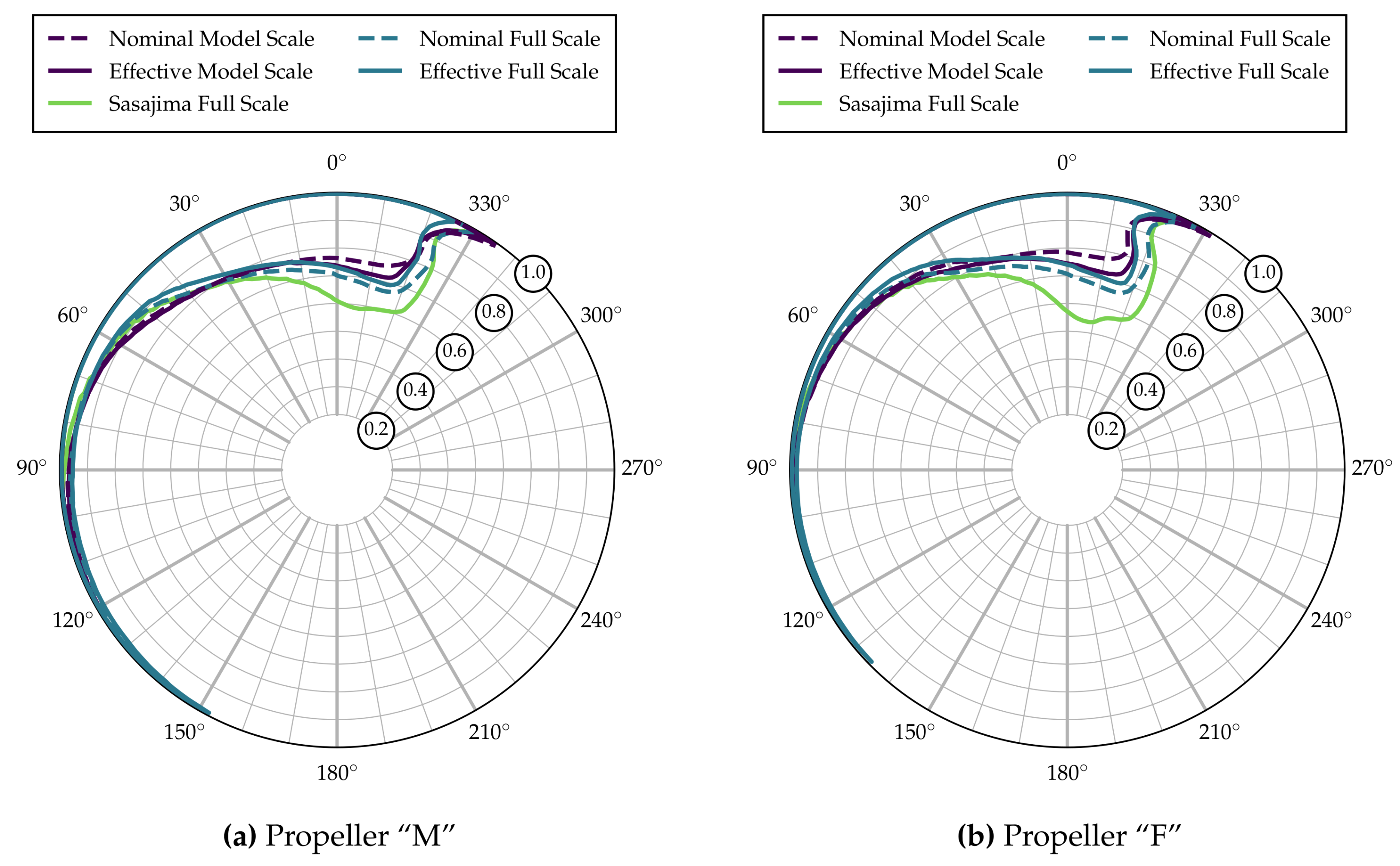
Figure 3a gives an overview over the global differences in sheet cavitation over one revolution. The lines indicate the radial extent of sheet cavitation for all blade angles in the different wakes. The lower cutoff threshold for these plots is a cavity thickness of 5% of the blade section thickness at .
As can be seen from Figure 3a, there is little variation in cavitation inception angle (around 330) yet noticable variation in terms of radial extent between the five wake fields over a relatively wide range of blade angles. The nominal wake distribution at model scale clearly results in the smallest cavitation extent, underpredicting the extent seen in the full scale effective field, especially at the blade angles with maximum cavitation extent. Using the full scale distribution obtained by Sasajima’s method, the extent is overpredicted significantly, which is not surprising given the wake field seen in Figure 1e. The other three curves—representing the effective distribution at model scale and the two full scale fields—result in remarkably similar extents. There also appear to be differences in the closing behavior of the cavity, as can be seen from Figure 3a in the range 30–90.
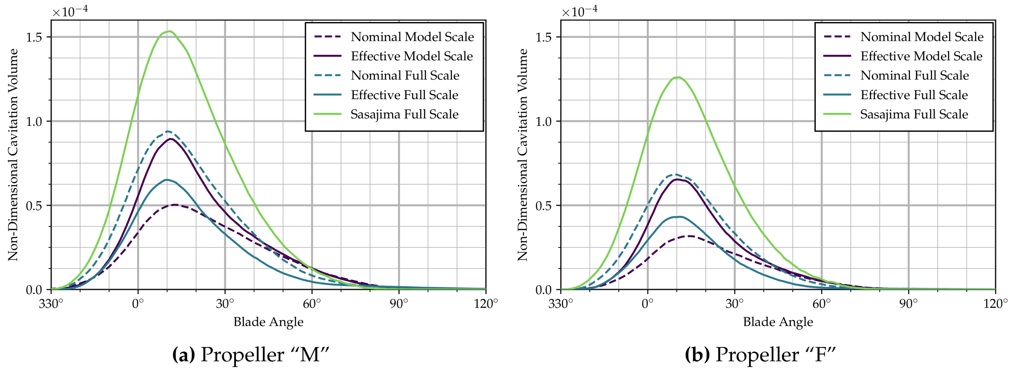
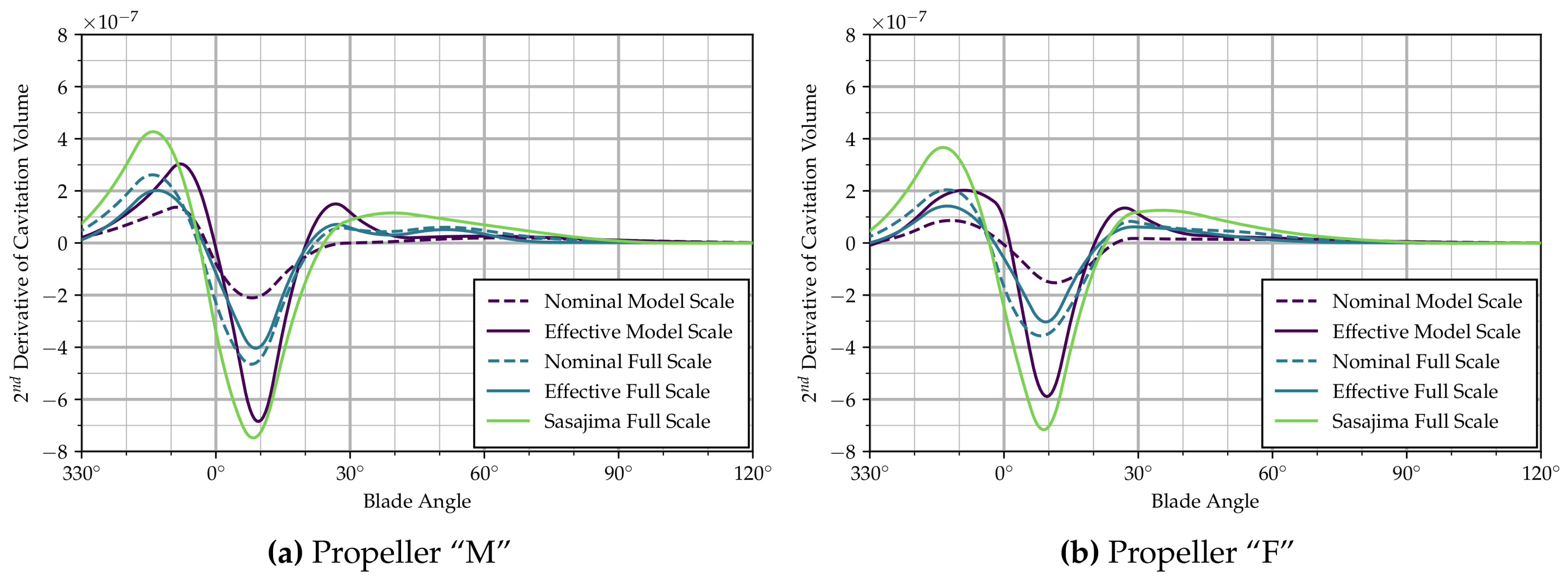
The time-variation in sheet cavitation is more easily quantified by looking at the cavity volume on one blade (non-dimensionalized by ), as shown in Figure 4a. Confirming the general trends between the wakes visible in Figure 3a, the small differences in inception and closure angle and large differences in maximum cavitation extent appear more clearly from Figure 4a. The plot also already indicates that the time-derivatives of the cavity volume are rather different between wake distributions when the cavity is shrinking between approx. 10–70 blade angle, hinting at major differences in associated hull pressure pulses. The second derivative of a B-Spline interpolation of the cavity volume with respect to blade angle (or time) is shown in Figure 5a.
Disregarding the curve corresponding to the field scaled by Sasajima’s method, particularly large differences exist between the results based on the nominal model scale distribution and the other computed curves. In that inflow field, the maximum cavity volume is more than 20% smaller than for the same propeller in the full scale effective wake distribution. In addition, second derivatives of the cavity volume (see Figure 5a) appear to be considerably different, the nominal model scale distribution again resulting in the smallest amplitudes.
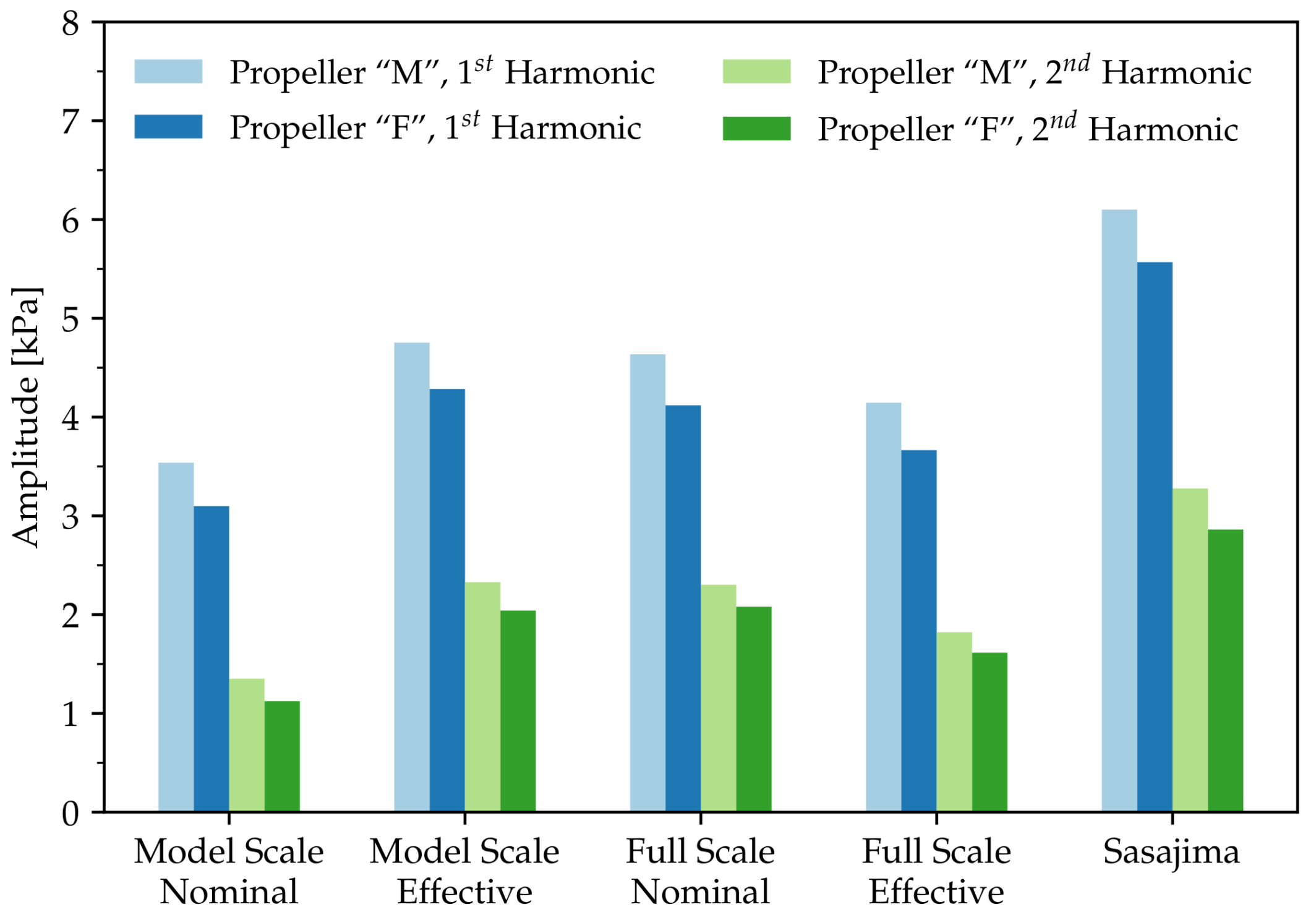
Hull pressure pulses are evaluated in a single point, located on the centerline, 17% of the propeller diameter above the propeller plane. These calculations were done in the BEM part of the simulation, applying the Bernoulli equation at an offbody point and Fourier-transforming the time signal. The results are given in Figure 6, which provides the amplitudes at first and second harmonic of the blade frequency. The pressure pulse results also reflect the findings described previously. For example, in the full scale effective wake distribution, the value for the first harmonic is 17% larger than in the nominal distribution at model scale. The differences are even larger for the second harmonic. Higher harmonics have not been evaluated for this paper, as the driving factors, such as tip vortex cavitation, are not captured or modeled in the present propeller analysis method.
5. Results for Alternative Propeller Design
For the purpose of the analyses described in this paper, two simple conventional propellers have been designed for the bulk carrier case mentioned in Section 3. Resistance and thrust deduction values from model tests (which were carried out for the hull used in the present computations, but with minor aftbody modifications) establish the thrust requirement for the propeller design. For the design point, the predicted full scale effective wake fraction (based on self-propulsion model tests with a stock propeller) of is used.
For the propeller design, a lifting line-based propeller design tool is employed that finds the optimum radial circulation (load) distribution for a circumferentially averaged wake field and required thrust. Radial pitch and camber distributions can then be found from the circulation distribution, assuming a standard NACA66 profile. Based on the designer’s experience, the propeller was chosen to be 3-bladed with moderate skew and no rake. The expanded blade area ratio was selected as .
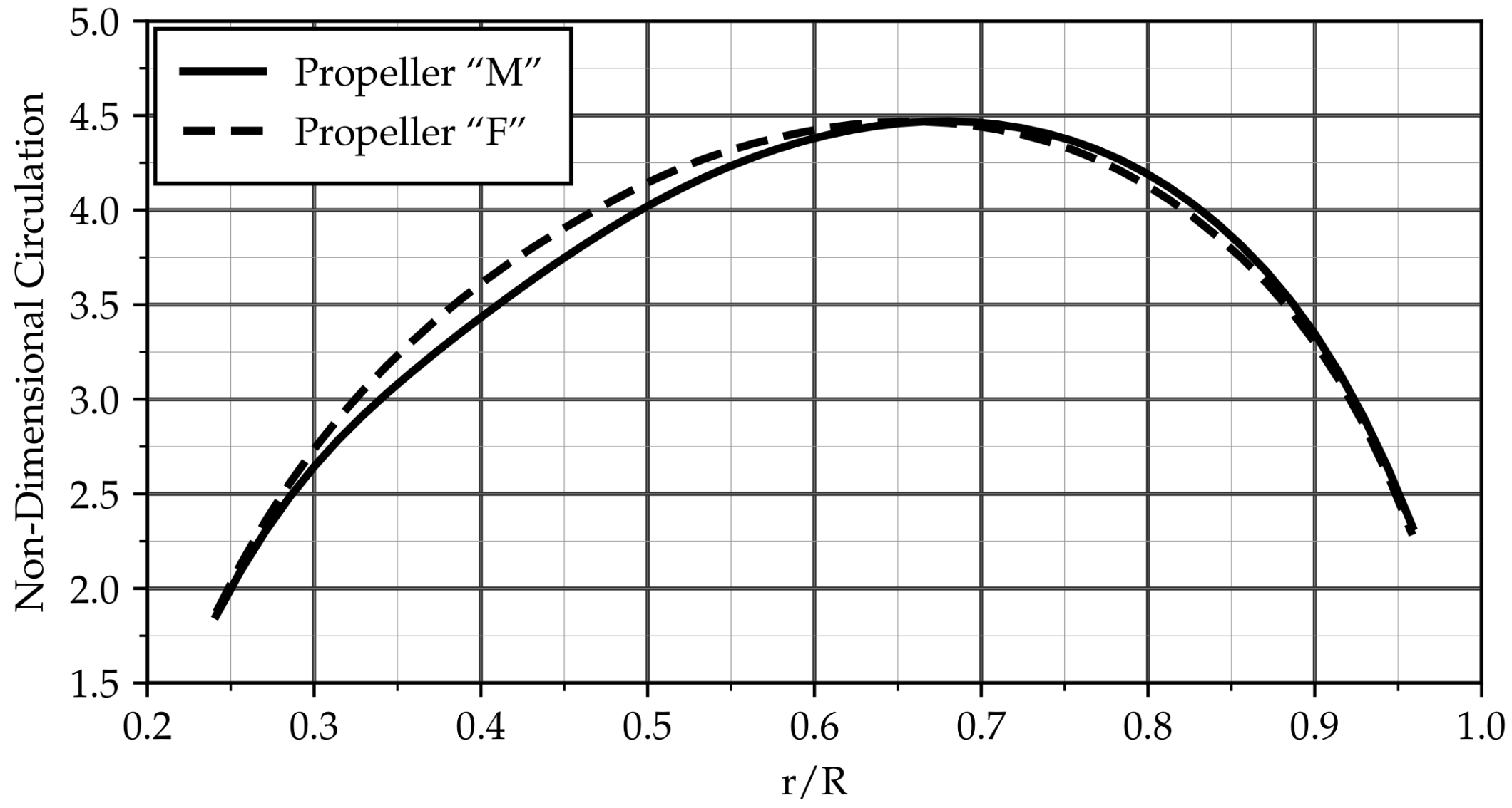
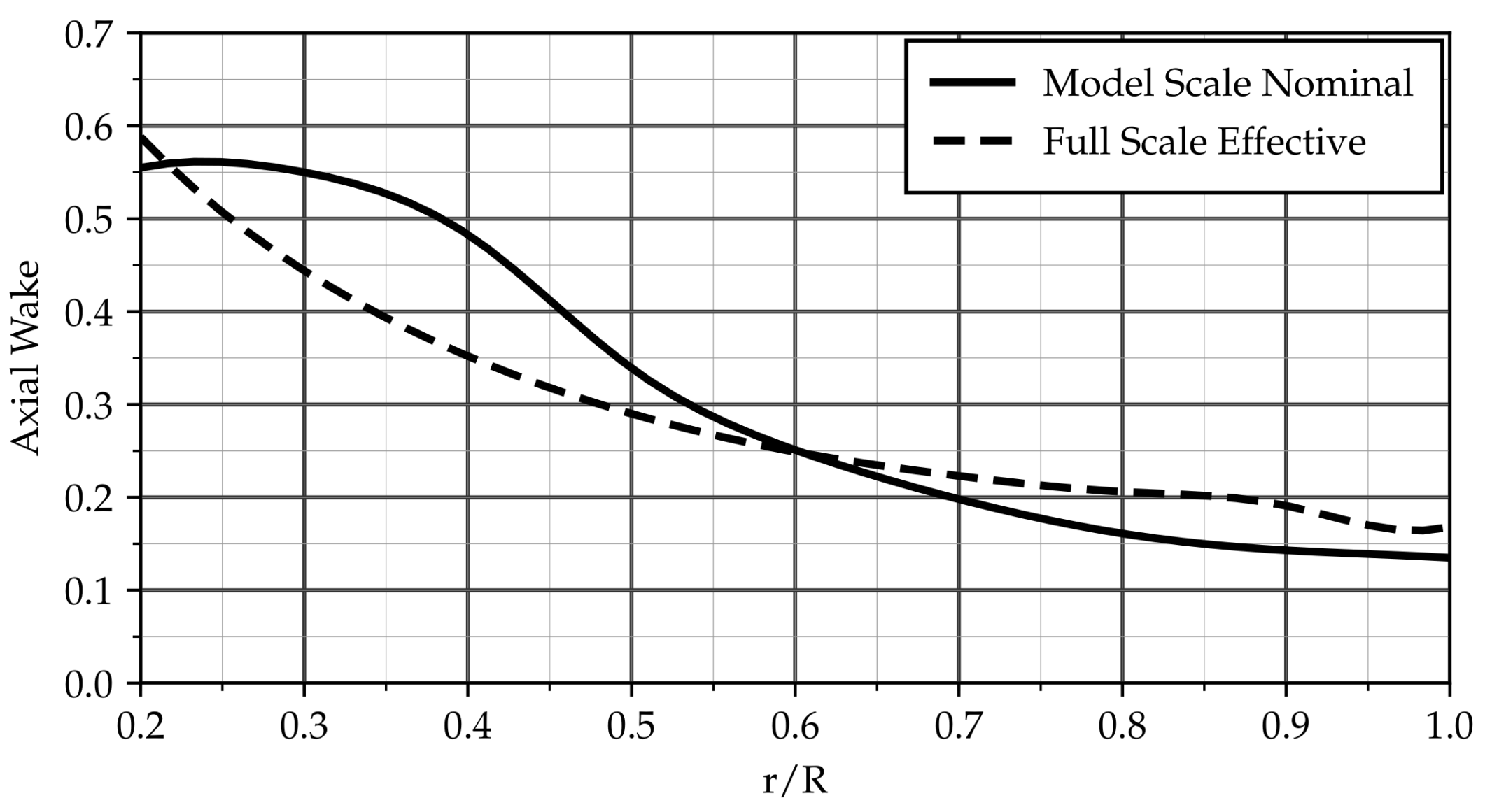
The nominal wake field obtained from Shipflow-XCHAP (see Figure 1a) is circumferentially averaged and scaled to the target effective wake fraction. This circumferentially averaged and scaled nominal wake field at model scale (which still varies radially, see Figure 7) is then used as input for the design tool. The optimum radial distribution of circulation found from lifting line theory for this case is shown in Figure 8. The corresponding propeller—which is the basis for all cavitation analysis results discussed so far—is referred to as Propeller “M” (as it is based on the model scale nominal wake).
Using this propeller, numerical self-propulsion simulations have been carried out to find the effective wake fields at model and full scale shown in Figure 1b,d, using the method described in Section 2.2.
In order to study the effect of nominal vs. effective wake on propeller design and resulting differences in propeller cavitation performance, the same design process is repeated with the full scale effective wake distribution as input, yielding Propeller “F”. Other input parameters, such as design wake fraction, advance ratio, number of blades, and blade area ratio, remain unchanged. The circumferentially averaged axial inflow for this case and the resulting radial circulation distribution are shown as dashed lines in Figure 7 and Figure 8. An inward shift of the loading compared to Propeller “M”—corresponding to the difference in inflow—can be seen from the latter.
The differences in effective wake distribution due to differences in geometry and radial load distribution between Propellers “M” and “F” are assumed to be negligible.
It can be seen from Figure 3b as well as Figure 4b that the characteristics of sheet cavitation extent and behavior of Propeller “F” are generally similar to Propeller “M”. The magnitudes of all values, however, are significantly lower. The cavitation volume in the full scale effective distribution is reduced by more than 30%, compared to Propeller “M”. Similar trends can be seen for the second cavity volume derivatives in Figure 5. Corresponding reductions in pressure pulses appear from Figure 6.
6. Conclusions
For the examined case of a modern and representative full-form ship, using the model scale nominal wake distribution for propeller design and cavitation analysis leads to a significant underprediction of cavitation extent, volume, and pressure pulses, compared to the behavior of the same propeller in the full scale effective wake field. Therefore, a conservative design is required if the propeller designer only has access to the measured nominal wake field. Otherwise, the expected extent of cavitation and acceptable levels of pressure pulses might be exceeded in full scale.
Compared to the propeller designed on the basis of the nominal wake in the model scale, the propeller designed for the effective full scale wake distribution performs better in all cavitation criteria considered. This highlights the importance of accurate wake data and the benefits of those—or hull geometry information—being available to the propeller designer. Knowing the effective wake distribution at full scale allows for a more realistic cavitation prediction in the propeller design process, enabling more efficient propeller designs.
Acknowledgments
The study was primarily funded by the Department of Mechanical Engineering at the Technical University of Denmark. The early development and implementation of the methods described in this paper were partly funded by Innovation Fund Denmark through the “Major Retrofitting Technologies for Containerships” project. Yasaman Mirsadraee’s PhD project is supported by Innovation Fund Denmark under the Industrial PhD programme.
Author Contributions
P.B.R. and Y.M. developed and implemented the sheet cavitation model in the panel code, continuing earlier work by P.A. and others. P.B.R. developed and implemented the RANS-BEM coupling. Y.M. designed the propellers used for this study. P.B.R. ran the RANS-BEM simulations and the subsequent BEM simulations. The results were further analyzed and discussed by all authors. P.B.R. wrote the paper with continuous input and comments from Y.M. and P.A. P.A. initiated and supervised the project.
Conflicts of Interest
The authors declare no conflict of interest.
References
- Jessup, S.; Mewis, F.; Bose, N.; Dugue, C.; Esposito, P.G.; Holtrop, J.; Lee, J.T.; Poustoshny, A.; Salvatore, F.; Shirose, Y. Final Report of the Propulsion Committee. In Proceedings of the 23rd International Towing Tank Conference, Venice, Italy, 8–14 September 2002; Volume I, pp. 89–151. [Google Scholar]
- Fu, T.C.; Takinaci, A.C.; Bobo, M.J.; Gorski, W.; Johannsen, C.; Heinke, H.J.; Kawakita, C.; Wang, J.B. Final Report of The Specialist Committee on Scaling of Wake Field. In Proceedings of the 26th International Towing Tank Conference, Rio de Janeiro, Brazil, 28 August–3 September 2011; Volume II, pp. 379–417. [Google Scholar]
- Sasajima, H.; Tanaka, I. Report of the Performance Committee, Appendix X: On the Estimation of Wake of Ships. In Proceedings of the 11th International Towing Tank Conference, Tokyo, Japan, 11–20 October 1966; pp. 140–144. [Google Scholar]
- Van Terwisga, T.; van Wijngaarden, E.; Bosschers, J.; Kuiper, G. Achievements and Challenges in Cavitation Research on Ship Propellers. Int. Shipbuild. Prog. 2007, 54, 165–187. [Google Scholar]
- Bosschers, J.; Vaz, G.; Starke, B.; van Wijngaarden, E. Computational analysis of propeller sheet cavitation and propeller-ship interaction. In Proceedings of the RINA Conference “MARINE CFD2008”, Southampton, UK, 26–27 March 2008. [Google Scholar]
- Gaggero, S.; Villa, D.; Viviani, M.; Rizzuto, E. Ship wake scaling and effect on propeller performances. In Developments in Maritime Transportation and Exploitation of Sea Resources; CRC Press: London, UK, 2014; pp. 13–21. [Google Scholar]
- Kinnas, S.A.; Fine, N.E. A Numerical Nonlinear Analysis of the Flow Around Two- and Three-dimensional Partially Cavitating Hydrofoils. J. Fluid Mech. 1993, 254, 151–181. [Google Scholar] [CrossRef]
- Fine, N.E. Nonlinear Analysis of Cavitating Propellers in Nonuniform Flow. Ph.D. Thesis, Massachusetts Institute of Technology, Cambridge, MA, USA, 1992. [Google Scholar]
- Vaz, G.; Bosschers, J. Modelling Three Dimensional Sheet Cavitation on Marine Propellers Using a Boundary Element Method. In Proceedings of the 6th International Symposium on Cavitation (CAV2006), Wageningen, The Netherlands, 11–15 September 2006. [Google Scholar]
- Vaz, G.; Hally, D.; Huuva, T.; Bulten, N.; Muller, P.; Becchi, P.; Herrer, J.L.R.; Whitworth, S.; Mace, R.; Korsström, A. Cavitating Flow Calculations for the E779A Propeller in Open Water and Behind Conditions: Code Comparison and Solution Validation. In Proceedings of the 4th International Symposium on Marine Propulsors (smp’15), Austin, TX, USA, 31 May–4 June 2015; pp. 330–345. [Google Scholar]
- Hally, D. Propeller Analysis Using RANS/BEM Coupling Accounting for Blade Blockage. In Proceedings of the 4th International Symposium on Marine Propulsors (smp’15), Austin, TX, USA, 31 May–4 June 2015; pp. 297–304. [Google Scholar]
- Rijpkema, D.; Starke, B.; Bosschers, J. Numerical simulation of propeller–hull interaction and determination of the effective wake field using a hybrid RANS-BEM approach. In Proceedings of the 3rd International Symposium on Marine Propulsors (smp’13), Tasmania, Australia, 5–7 May 2013; pp. 421–429. [Google Scholar]
- Regener, P.B.; Mirsadraee, Y.; Andersen, P. Nominal vs. Effective Wake Fields and their Influence on Propeller Cavitation Performance. In Proceedings of the 5th International Symposium on Marine Propulsors (smp’17), Helsinki, Finland, 12–15 June 2017; pp. 331–337. [Google Scholar]
Figure 1.
Wake fields for cavitation analysis, all scaled to .

Figure 2.
Potential wake field.

Figure 3.
Radial cavitation extent.

Figure 4.
Cavitation volume.

Figure 5.
Second derivatives of cavitation volume.

Figure 6.
Pressure pulse amplitudes.

Figure 7.
Circumferentially averaged axial velocities used for propeller design.

Figure 8.
Radial circulation distributions.

Table 1.
Wake fractions before scaling.
| Wake Field | Axial Wake Fraction |
|---|---|
| Nominal Model Scale | 0.360 |
| Effective Model Scale | 0.300 |
| Nominal Full Scale | 0.240 |
| Effective Full Scale | 0.237 |
| Sasajima Scaling | 0.236 |
| Target Value | 0.250 |
© 2018 by the authors. Licensee MDPI, Basel, Switzerland. This article is an open access article distributed under the terms and conditions of the Creative Commons Attribution (CC BY) license (http://creativecommons.org/licenses/by/4.0/).
Share and Cite
MDPI and ACS Style
Regener, P.B.; Mirsadraee, Y.; Andersen, P. Nominal vs. Effective Wake Fields and Their Influence on Propeller Cavitation Performance. J. Mar. Sci. Eng. 2018, 6, 34. https://doi.org/10.3390/jmse6020034
AMA Style
Regener PB, Mirsadraee Y, Andersen P. Nominal vs. Effective Wake Fields and Their Influence on Propeller Cavitation Performance. Journal of Marine Science and Engineering. 2018; 6(2):34. https://doi.org/10.3390/jmse6020034
Chicago/Turabian StyleRegener, Pelle Bo, Yasaman Mirsadraee, and Poul Andersen. 2018. "Nominal vs. Effective Wake Fields and Their Influence on Propeller Cavitation Performance" Journal of Marine Science and Engineering 6, no. 2: 34. https://doi.org/10.3390/jmse6020034
Note that from the first issue of 2016, this journal uses article numbers instead of page numbers. See further details here.